Submitted:
22 January 2025
Posted:
23 January 2025
You are already at the latest version
Abstract
To achieve different compression rates for images while preserving important regions, a semantic network-based deep residual variational auto-encoder is introduced in this paper. The network is divided into two components, a semantic analysis network and an image compression network. The former evaluates the importance of image pixels and accurately locates important semantic regions and key information in the image. According to the semantic importance of different regions, the encoding strategy is dynamically adjusted. The latter utilizes a deep residual variational autoencoder to efficiently encode and decode images, while combining Lagrange multipliers to adjust the model flexibly and the weights of the bitrate. With this model, multiple compression rates have been implemented. Quality of reconstruction achieves better performance with compression at different rates. Finally, a semantic loss function is proposed to replace traditional compression loss functions. Extensive experiments conducts on several datasets, including the Kodak, CLIC and Tecnick TESTIMAGES, which were public datasets. Results demonstrate that our method can effectively improve the quality of image reconstruction at various compression rates. Compared with traditional methods, the peak signal-to-noise ratio is increased by an average of 2dB at the same bitrate, and the structural similarity index is the most close to 0.998. The subjective visual quality is better, especially when processing complex scene images, which can better preserve the details and textures of key objects. This approach can effectively avoid common distortions such as block effects and blurring in traditional methods.
Keywords:
lossy image compression
; variational auto-encoder
; semantic networks
; variable rate compression
1. Introduction
With the explosive growth of digital images and videos, the storage and transmission of image data have become major challenges in information processing. Image compression techniques effectively address this issue by reducing the redundancy of image data. These techniques can be broadly categorized into lossless and lossy compression. Lossless compression removes statistical redundancy from the image in a reversible process, typically used in scenarios where image clarity is paramount. In contrast, lossy compression algorithms process image information based on the principle that the human eye is insensitive to certain visual features, often resulting in irreversible data reduction.
Many innovative compression methods, such as JPEG [1], JPEG 2000 [2], and BPG [3], have been used widely. Traditional image compression methods focus on pixel-level information, reducing data volume through transform domain coding and quantization. However, these methods often overlook the semantic information of the image content, such as the importance and visually perceived characteristics of different regions. For instance, in a landscape photograph, the sky and grass may not be as significant as buildings or people, yet they are often treated equally in conventional compression methods.
Recently, with the continuous development of computer vision, semantic segmentation has emerged as a research hotspot, with its core role being to assign each pixel in an image to a specific category, thereby clearly distinguishing different objects and regions in the image. This technology has been widely used in many fields such as automatic driving, medical image analysis, and scene understanding. For example, in the medical field, various semantic segmentation techniques [4,5,6] can assist doctors in identifying lesion regions in computed tomography or nuclear magnetic resonance imaging scan images to improve the accuracy of diagnosis. As deep learning technology advances, the role of semantic information in image compression has become increasingly significant. Image compression technology leverages semantic information to distinguish between different regions in an image. Given the varying importance of various regions to the human visual system, by identifying the semantic information in the image, the compression algorithm can adjust the compression rate in a more targeted way. High pixel quality can be maintained for important image elements such as faces or texts, while the compression level can be increased for less critical elements like backgrounds or minor details, reducing the overall data volume. This content-based adaptive compression strategy not only optimizes storage and transmission efficiency but also ensures the quality of key information in terms of visualization.
Conventional compression methods generally take the input image and a conventional transform lossy coding method performs the transform . The transform so obtained is represented as a discrete-valued vector after quantisation to achieve. For storage or transmission, the vectors are binaryised and serialised into an entropy coded bit stream to reduce the statistical redundancy therein. In the decoding process, the opposite step is performed, i.e., dequantisation , followed by an inverse transformation to reconstruct the output image . The key components of an image codec include an encoder, which transforms the original image into a more compressible representation, and a decoder, which reconstructs the image from a possibly quantized version of that new representation. Some commonly used image codecs include JPEG, JPEG2000, PNG [7] and FLIF [8].
Deep learning has made significant strides in the field of image compression, often outperforming traditional codecs in terms of both compression efficiency and image quality. In 2020, Yang et al. [9] proposed a variable R-D optimization method using a modulated auto encoder, which significantly enhances R-D performance. However, this approach necessitates a more complex training strategy to coordinate the joint training of the auto encoder and the modulation network. In 2021, Hu et al. [10] enhanced entropy estimation and signal reconstruction by introducing a super-prior model, thereby improving the compression efficiency of high-resolution images. However, their method did not fully consider decoding speed and computational efficiency. In 2022, He et al. [11] proposed an inhomogeneous channel-conditional adaptive coding method, which improves coding efficiency without sacrificing speed by incorporating a spatial-channel context model. However, this method lacks adaptability to different compression rates. In 2023, Tong et al. [12] defined a vector of quantization regulators coupled to predefined Lagrange multipliers to control quantization errors across all potential representations of discrete variable rates. The reparameterization approach made the model compatible with circular quantizers but was not sufficiently flexible in adapting to diverse compression requirements. In 2024, Sebai et al. [13] proposed a new depth map compression model that uses an optimized convolutional neural network to extract features from depth maps, combined with the VGG19 model and a wedge filter to differentiate between depth maps and texture images using deep feature classification techniques. However, this model does not apply to a wide range of image types. Yang et al. [14] proposed an end-to-end optimized lossy image compression framework for diffusion generative models, which relies on a transformational coding paradigm. This paradigm maps the image into potential space for entropy coding and then back into data space for reconstruction. However, this approach could potentially compromise the deterministic and predictable nature of the compression. Therefore, developing compression ratios that can be dynamically adjusted to balance image quality and transmission bandwidth is crucial for achieving efficient data storage and transmission.
Semantic analysis is crucial in image compression. Traditional image compression methods typically focus solely on pixel-level information, often ignoring the semantic content of the image. This oversight can lead to unsatisfactory compression results. In contrast, image compression methods that leverage semantic networks can apply different compression strategies to various semantic regions, thereby achieving superior compression outcomes. For instance, a stricter compression strategy might be applied to background areas, while a more lenient approach could be reserved for critical regions such as characters and text. This nuanced approach can enhance both the quality and usability of the image.
Most existing codecs do not explicitly utilize high-level semantics during encoding or decoding. Prakash et al. [15] proposed methods for content-weighted bit rate control, but these did not explicitly harness high-level semantics. Agustsson et al. [16] explored the use of semantics in image compression, albeit in a limited context. Their approach employed semantic considerations in bit rate allocation, but only within a somewhat constrained setup, necessitating user intervention to prioritize certain semantic regions over others. Wang et al. [17] employed a convolutional neural network (CNN) to analyze the semantic regions of an image. This analysis can be used to determine compression iterations for each image block once a semantic importance map is generated. While this method eliminates the need for retraining the model to adapt to different rates, it necessitates the creation of a separate, standalone model, which can consume significant memory resources. Akbari et al. [18] introduced a deep semantic segmentation-based layered image compression framework. This framework uses a segmentation map and a compressed image to create an initial reconstruction of the image, encoding the difference between the input image and the initial reconstruction into an enhancement layer. Although the architecture is designed to compress the image and extract its semantic information concurrently, it does not prioritize preserving semantic information during compression. Instead, it focuses on embedding semantic information during the compression process to prevent the duplication of semantic information generation in client applications.
Generally, the human eye pays varying degrees of attention to different regions of an image. For example, in a portrait, the sharpness and texture details of the foreground subject are more noticeable than the background. However, current image compression techniques often apply uniform processing to every pixel, leading to a suboptimal allocation of compression bits, particularly in images where the background is of lesser importance. Therefore, developing techniques that enable more efficient compression bit allocation, based on a clear distinction between foreground and background, is essential for optimizing image compression.
To archive target above, a variable rate image compression network based on semantic information has been proposed. It first generates relevant semantic regions through a semantic analysis network and then computes compression levels for each region which are subsequently used by the image compression network. Main contributions of this approach are as follows.
(1) A semantic network-based deep residual variational auto-encoder is proposed for image compression. This approach includes a carefully designed compression bit allocation algorithm that computes the appropriate compression level for each image block. By integrating the outcomes of semantic analysis, the image is compressed in a way that prioritizes the retention of significant visual details while minimizing the file size.
(2) A single-model multi-compression-rate adaptive image compression framework is proposed, which achieves an effective trade-off between compression rate and image quality within multiple ranges of γ-values through the introduction of a variable compression rate module and optimization of the Lagrange multiplier γ-value, thus significantly improving the flexibility and applicability of the model and meeting the diverse needs of different users for image compression.
(3) A semantic-based multinomial loss function is proposed to guide the training of image compression networks, realizing that one network model produces data outputs with different compression ratios.
To verify the methods performance of above, some experiment on multiple datasets has been run. The rest of the paper is organized as follows. We have introduced three modules proposed in detail in section 2, which includes in the semantic analysis module, adaptive variable compression rate module, and semantic enhancement image compression module. To verify these methods, some numerical experiments have been discussed in section 3, where shows results and a comparison of other methods. Finally, summarizes this approach and future research shows in last section.
2. Principal of Proposed Method
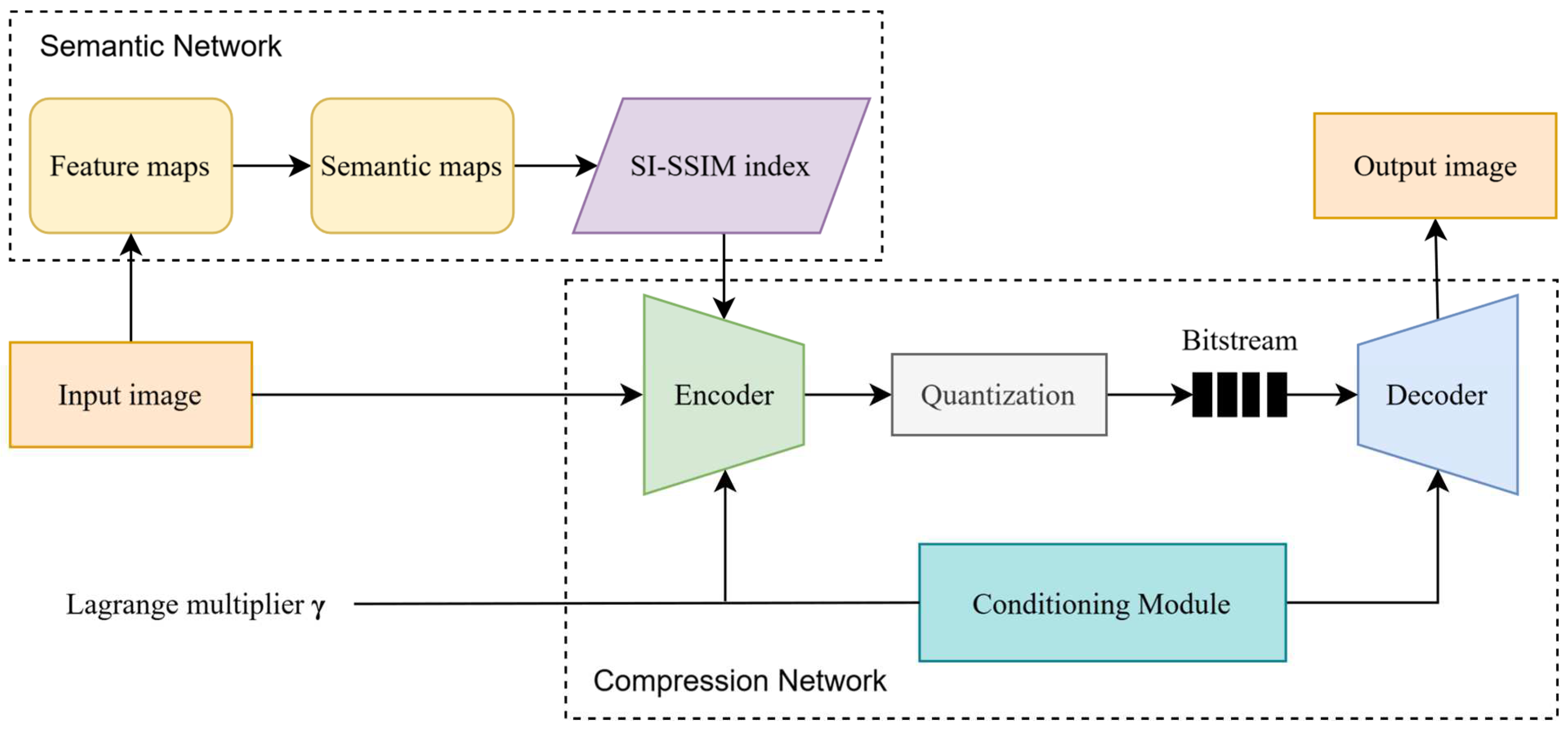
We propose a method to optimize image compression by the importance of image content, and the overall framework is shown in Fig. 1. The method includes the following aspects.
(1) Semantic analysis module
This module analyzes the image content and identifies the key semantic information to provide the necessary contextual information for image compression to maintain the clarity of the important content in the process.
(2) Adaptive variable compression rate module
Through the Lagrange multiplier adjustment strategy, the module can optimize a variety of compression ratios in a single model, which ensures that the best compression effect can be achieved in different application scenarios.
(3) Semantic enhancement image compression module
It uses information from the semantic analysis module to guide image compression, ensuring that important semantic content remains clear after decompression while allowing more degrees of freedom in compressing unimportant parts to improve compression efficiency.
Figure 1.
Overall architecture of the proposed method concluding in three parts, semantic network, adaptive variable compression rate module, and semantic enhancement image compression module.
Figure 1.
Overall architecture of the proposed method concluding in three parts, semantic network, adaptive variable compression rate module, and semantic enhancement image compression module.
2.1. Semantic Analysis Module
The semantic analysis module utilizes a classification-based architecture to identify regions that attract the human eye's visual attention. It strategically allocates more compression bits to these areas, facilitating differential image compression. As depicted in Figure 2, the semantic analysis module structure comprises several key components, including a convolutional layer, a fully connected layer, a softmax layer, a global average pooling(GAP)layer, and a rectified linear unit(ReLU) activation layer.
In Figure 2, the convolutional layer comprises a total of five sets of convolutions designed for extracting image features. Let F represent the final convolution, which outputs several feature maps. Each feature map is capable of capturing a distinct type of feature present in the original image. The fully connected layer then transforms these feature maps into a one-dimensional feature vector. The output of the fully connected layer is denoted as Z, commonly referred to as logits. This relationship is formalized by
where Z is the output of the fully-connected layer and each element corresponds to the original predicted score for a category, W is the weight matrix, F is the output of the convolutional layer, and is the bias term.
Assuming that a category is defined as C, the linear prediction score of category C is denoted by yC. The output Z of the fully connected layers is the input to the softmax function, which converts logits into a probability distribution. This process is described as follows.
where P(yC) is the predicted probability of category , ZC is the logit of category C, and M is the total number of categories.
The softmax layer transforms the output of the fully connected layer into a probability distribution. It selects a particular category based on these output probabilities and calculates the gradient of the predictions for the selected category concerning the feature map from the final convolutional layer. This calculation determines the contribution of the feature map to the classification. In this paper, the gradient of each pixel is utilized to assess its contribution to the final prediction outcome. The specific formula for calculating this gradient, denoted as Grad presented by
where Fk is the feature map of the k-th channel of the convolutional layer. The global Average Pooling (GAP) is utilized to process each feature map Fk, thereby obtaining the importance weight for each feature map about category C. The specific formula for this calculation is presented as following, we have
where is the importance weight of each feature map for category C, H and W are the height and width of the feature map, respectively, is the feature map element.
The weights derived from the GAP layer are reassigned to the feature map to emphasize the parts that significantly influence the classification decision. The application of the ReLU activation function enhances the regions with positive correlations. To visualize the network’s impact on the original image, particularly for a specific class C, we employ a linear weighted sum of these weights and the feature map. This sum represents the probability that each pixel in the image belongs to class C.
By up-sampling HC the semantic map, this paper obtains the semantic importance map of the Kodak dataset through the semantic analysis network, as shown in Figure 3.
The intensity of highlighting reflects the level of semantic importance from figure. The darker the red in the heat map, the greater the contribution of that area to the model’s final prediction result, indicating a higher level of attention paid to that part of the image. The yellow portions of the image command the second highest level of attention. Conversely, the blue areas have minimal impact on target detection and recognition, and the model deems this information to be redundant.
2.2. Adaptive Variable Compression Rate Module
In recent years, deep neural networks have made remarkable achievements in image feature learning and representation learning, providing a new paradigm for image compression tasks. In this paper, we adopt a deep residual network-based image compression method that combines the advantages of a Residual Network (ResNet) [19] and Variable Auto-Encoder (VAE) [20], which is based on the unfolding under the benchmark model of Ballé et al. [21]. In the following paper, we will start the discussion from the Variational Auto-Encoder VAE.
VAE is a generative model that integrates the architecture of an auto-encoder with the principles of variational inference. This combination enables the modeling of complex data distributions by learning the data’s latent representation. The VAE is composed of two main components: an encoder and a decoder. Its overarching objective is to learn a probabilistic distribution that facilitates the generation of data. Let x be a random variable representing the data (in this paper, the original image) with an unknown data distribution pθ(x). In VAE, it is difficult to model pθ(x) directly from x, so the data distribution is modeled by introducing a simpler prior distribution pθ(z). The latent variable z is first sampled from the simple distribution, and the reconstructed image is generated using the latent variable z. This is obtained according to Bayes’ formula.
where θ is a model parameter. Since pθ(z|x) is difficult to solve, so in this paper qΦ(z|x) design distribution to approximate the pθ(z|x) distribution, using KL dispersion to fit the similarity of the two distributions with the following.
The training objective of the VAE is to minimize the variational upper bound on the negative log-likelihood.
where x is an image. By minimizing the overall loss function Ltotal, the VAE model can learn the latent representations while maintaining an efficient reconstruction of the original data and making the distribution of the learned latent representations closer to the standard normal distribution.
To model high-dimensional data such as images, hierarchical Variational Auto-Encoders (VAEs) have been proposed. These models enhance the flexibility and expressiveness inherent in VAEs. In this paper, we employ the ResNet VAE network model, an auto-encoder structure that leverages the architecture of a Residual Network. By incorporating residual connections, ResNet facilitates the learning of identity mappings, thereby mitigating the issue of gradient vanishing. In the context of image compression, ResNet-based auto-encoders construct deep architectures by stacking residual blocks. This approach enables them to more effectively capture and encode high-level features within the image.
The ResNet VAE is a hierarchical VAE that uses a set of latent variables denoted , where H is the total number of variables in an autoregressive fashion.
where z<H denotes {z1,z2,...,zH-1}. Typically, z1 has fewer dimensions and zH has larger dimensions. The architecture from low to high dimensions not only improves the flexibility of the VAE but also captures the coarse to-fine nature of the image.
In the ResNet VAE network, the posterior and prior have the following form, we have
and
Inserting this into the VAE objective function equation (8) gives the ResNet VAE objective function, we have
For lossy compression, the form of the likelihood distribution, pX|Z(‧), depends on which distortion measure is used, d(‧). Typically, this is defined by
where λ is the standard hyperparameter and is the reconstructed image, which depends on all the latent variables . In image compression, d(‧) is usually chosen to be the mean square error (MSE), in which case the data likelihood forms a (conditional) Gaussian distribution.
The objective function of the ResNet VAE network model is finally obtained by
The image compression network adopts the network architecture from the literature [22]. In the encoder part, five levels of features are extracted from the image and sent to the latent variable blocks in the decoder to produce a compressed bit stream, and the overall architecture is shown in Figure 4. Each latent variable block indexed by i contains the latent variable zi as well as the posterior qi and prior pi, and each latent variable produces a separate sequence of bits during encoding, and the set of all such sequences forms the final bitstream of the input image. In the middle of Figure 4 is the residual network block section, which consists of a deep convolutional network, layer normalization, and an activation function GELU. Individual models are trained to operate on a range of ratios by accepting γ as an input to the model, and all a posteriori and priori are conditioned on γ.
The conditioning module comprises two fully connected (FC) layers and ReLU and GELU activation functions. The goal is to learn the complex relationship between γ and model weights to generate appropriate weights for different compression rates. The objective of training the variable rate module is to optimize the conditional a posteriori qi(zi|x,z<i,γ) and the conditional priori pi(zi|x,z<i,γ) by randomly sampling γ from a continuous range of values [γlow,γhigh] throughout the training process. By adding a Lagrangian parameter γ to the image compression, the variable rate loss function is defined by
where γ is a variable rate sampling strategy throughout the training process. Once a model has been trained, it is possible to adjust the distortion rate using a single model by simply changing the γ input to the model.
2.3. Semantic Enhancement Image Compression Module
The semantic importance mapping of each pixel can be obtained through Section 3.2, and the self-information weighted SSIM (SI-SSIM index [23]) is computed from the semantic map, a process that helps in evaluating the compressed image for optimization of the compression ratio while preserving the quality of semantically important regions. Given an input image size of H×W, the image is divided into N blocks of size 8×8 each, then .
Let be the average compression level of the image, and the compression level of block i is Mi. To ensure the consistency of the compression ratio, the sum of the compression levels of all image blocks should be defined as
Converting the semantic importance mapping to a greyscale map, the higher the semantic importance of a pixel (x,y), the higher its greyscale g(x,y), and the higher the probability that i belongs to a semantic category of interest to the human eye. Let the semantic importance value Vi of block i be the sum of the corresponding grey values g(x,y) of each pixel (x,y) belonging to the block, with the following form.
The semantic level Li of a block is then defined as
Considering that the sum of the compression levels of the blocks is , the computed compression level of block i can be expressed as Ti.
SI-SSIM is structural similarity based on semantic importance (SSIM). It is actually the average sum of SSIM corresponding to each block i, weighted by the semantic level Li. SI-SSIM is defined as
where and are the original and reconstructed images; xi and are block i in images x and , respectively.
The encoder and decoder contain θ and Φ parameters, and the final loss function of Equation (15) is a multinomial loss distribution, defined as
To perform discriminative compression, D, the distortion between x and in (12) is measured using the SI-SSIM already defined in (11), which is used to train the network model as part of the loss function, which allows it to adaptively allocate more bits to the semantically most important regions of the image. The multinomial loss can be defined as
where γ is one of the inputs to the model, allowing the model to adjust between different rate-distortion points after semantic analysis.
3. Experimental Results
3.1. Dataset and Implementation details
Datasets: In this paper, the Caltech 256 dataset [24], which contains 256 categories and a total of 30,607 images, is chosen to train the semantic analysis network. The COCO 2017 [25] dataset containing 118,287 images is selected to train the image compression network. To validate the performance of the proposed compression model, the model is evaluated on three public test sets: (1) the Kodak [26] test set contains 24 images with 512×768 or 768×512 pixels respectively. (2) The CLIC 2022 test set contains 30 images, approximately 2048×1365 pixels. (3) The Tecnick TESTIMAGES [27] test set uses RGB OR 1200×1200 segmentation and contains 100 images with 1200×1200 pixels.
Implementation details: In this experiment, the semantic network and image compression network adopt the Adam optimizer [28], with a batch size of 8 and 100 iterations. The learning rate is 10-4. Lagrange multiplier = {32, 64, 128, 256, 512, 1024, 2048}. The server is configured with an RTX 3090 GPU, the operating system is Ubuntu 22.04, the deep learning framework is pytorch 1.10.0, and the programming language is Python 3.9.
Metrics: We use standard metrics to quantify rate and distortion. The reconstruction distortion is measured by the peak signal-to-noise ratio (PSNR, higher is better).
where pixel values are between 0 and 1, and the MSE is measured in the RGB space.
We use the MS-SSIM measure of image quality, which calculates SSIM values on multiple scales and averages these values to obtain a final image quality score. The metric ranges from 0 to 1, with the closer to 1, the better the quality of the reconstructed image.
3.2. Comparison with traditional image compression methods
Table 1 shows the comparison results of PSNR and MS-SSIM indicators of five existing models and the model proposed in this paper on the Kodak dataset at a bit rate of 1.12, where the black bold font indicates the optimal indicator. Experiments show that the proposed method is superior to other traditional fixed-rate image compression methods.
We use methods such as JPEG, JPEG2000, BPG, TCM [29] , and INN [30] , and conducted comparative experiments based on three public datasets. The comparison on the Kodak dataset is shown in Figure 5, the comparison on the CLIC 2022 dataset is shown in Figure 6, and the comparison on the Tecnick TESTIMAGES dataset is shown in Figure 7. The method proposed in this paper is named Song method.
In these three sets of comparison figures, the black curve represents the compression method we proposed. Experimental results show that our model outperforms the traditional JPEG, JPEG 2000, and BPG methods in the key indicator of PSNR. In addition, although the methods of TCM and INN show certain competitiveness and are between JPEG and BPG, they still do not reach the performance level of our method. In the comparison of MS-SSIM indicators, our method performs best at all bit rates, which highlights its advantage in preserving image structural information. JPEG2000 and BPG also perform relatively well, but JPEG has a lower MS-SSIM value, which indicates that more structural information may be lost during image compression.
The superior performance of our method is due to its smarter allocation strategy of coding bits. Specifically, more compression bits are allocated to semantically important regions in the image, while sacrificing the reconstruction quality of those insignificant regions. Since the number of semantically important regions is usually less than that of unimportant regions in an image, this strategy enables our method to achieve higher compression efficiency while maintaining key information in the image.
3.3. Comparison with semantic deep learning based image compression methods
We select the methods of DSSLIC, EDMS [31], DeepSIC [32], and ADAPTIVE DIC [33] and conduct comparative experiments on three public datasets. These comparative methods have a high degree of similarity in structure with the semantic method proposed in this paper.
Table 2 shows the PSNR and MS-SSIM comparison results of four existing semantic image compression models and the proposed method in this paper on the Kodak dataset at a bit rate of 0.75, where the black bold font indicates the optimal index. From the perspective of PSNR and MS-SSIM indicators, the method of DSSLIC has a maximum PSNR of 39.8, but its MS-SSIM is slightly lower than other methods; the method of EDMS has a maximum MS-SSIM of 0.993 and a relatively low PSNR; the method of DeepSIC has an intermediate PSNR and MS-SSIM; the method of ADAPTIVE DIC has a PSNR close to the highest value and a high MS-SSIM, while the method proposed in this paper outperforms other methods in both PSNR and MS-SSIM, reaching 40.1 and 0.996 respectively, showing better performance.
Figure 8 shows the comparison of the indicators of the four semantic compression models and the method proposed in this paper on the Kodak dataset, Figure 9 shows the comparison of the indicators of the four methods and the method proposed in this paper on the CLIC 2022 dataset, and Figure 10 shows the comparison of the indicators of the four methods and the method proposed in this paper on the Tecnick TESTIMAGES dataset, where the black curve represents the method proposed in this paper.
It can be seen from the PSNR charts of the three sets of public data sets that the method proposed in this paper shows the highest PSNR value at different bit rates, showing its obvious advantage in image compression quality, especially in the low bit rate range. The performance of this method is similar to that of DSSLIC, but with the increase in bit rate, the advantage of this method is more obvious. The methods of EDMS and DeepSIC perform worse than other methods at all bit rates, and their PSNR values are relatively low. This shows that the method proposed in this paper has better performance and application potential in the field of image compression.
From the MS-SSIM charts of the three data sets, it can be seen that the proposed method outperforms the other four methods in the MS-SSIM index at different bit rates, showing its obvious advantage in image compression quality. With the increase in bit rate, the MS-SSIM values of all methods show an upward trend, but the growth rate and the final MS-SSIM value of the proposed method are higher than those of other methods, especially in the medium and high bit rate range, the gap between the proposed method and other methods is more obvious. In the low bit rate range, although the MS-SSIM values of each method are relatively close, the proposed method is still slightly better. The method of DSSLIC also performs well in medium and high bit rates, following closely behind the proposed method, while the method of EDMS , DeepSIC , and ADAPTIVE DIC performs relatively weakly in each bit rate range, and the MS-SSIM values are generally lower than those of the proposed method and the method of DSSLIC These results show that the image compression method proposed in this paper has better performance in maintaining image quality.
3.4. Comparison with variable rate image compression methods
The methods of MAE, Coarse-to-Fine, ELIC, and QVRF are selected for comparative experiments on three public datasets, among which the four methods are all variable rate methods. This paper selects methods with similar functions for comparison.
Figure 11 shows the indicator comparison of four variable rate image compression methods and the method proposed in this paper on the CLIC 2022 dataset, and Figure 12 shows the indicator comparison of the four methods and the method proposed in this paper on the Tecnick TESTIMAGES dataset, where the black curve represents the method proposed in this paper.
From the PSNR charts of the two datasets, it can be observed that the proposed method shows the highest PSNR value at all bit rates, which indicates that the proposed method can maintain high image quality in image compression. With the increase of bit rate, the PSNR values of all methods are improved, but the increase of the proposed method is more significant, especially in the medium and high bit rate range, and the advantage of the proposed method is more obvious compared with other methods. In the low bit rate range, although the PSNR values of the methods are not much different, the proposed method is still slightly better. The methods of QVRF and ELIC also perform well in medium and high bit rates, following the proposed method, while the methods of Coarse-to-Fine and MAE perform relatively poorly in various bit rate ranges, and the PSNR values are generally lower than other methods. From the MS-SSIM charts of the two datasets, it can also be seen that the proposed method achieves the best MS-SSIM value at all bit rates, showing its obvious advantage in image compression quality.
Table 3 shows the PSNR and MS-SSIM metrics for four models compared with the model proposed in this paper at a bit rate of 1.25. From the perspective of PSNR and MS-SSIM, the method proposed in this paper has achieved the best results in both indicators, with PSNR reaching 41.5 and MS-SSIM reaching 0.997, which shows that the method proposed in this paper has obvious advantages in image compression quality. In contrast, although the method of Coarse-to-Fine has a higher PSNR value of 41.2, it is slightly lower than the method of QVRF in MS-SSIM, while the method of QVRF performs best in MS-SSIM, reaching 0.995, but the PSNR value is slightly lower than that of Coarse-to-Fine The methods of MAE and ELIC perform relatively poorly in these two indicators, with PSNR and MS-SSIM values lower than other methods. Overall, the method proposed in this paper achieves the best balance in image compression quality, ensuring both a high PSNR value and an extremely high MS-SSIM value, showing its superior performance in the field of image compression.
3.5. Visual comparison
Figure 13 shows the visual evaluation comparison of JPEG, JPEG2000, BPG, and the proposed method. JPEG and JPEG2000 are prone to block effects after image decompression. This is because these two methods use block-based discrete cosine transform and embedded quantization strategies during the compression process, resulting in unnatural segmentation lines at the boundaries of image blocks after decompression. In contrast, although the BPG method has improved the block effect to a certain extent, it is still difficult to completely avoid the problem of blurred details. The proposed method allocates coding bits irregularly, distributing more compressed bits to areas of high semantic importance, which can effectively avoid block effects.
Figure 14 is a comparison of the details of the three methods in the range of 0.72bpp-0.76bpp. The image in the upper right corner of each figure is the magnified effect of the important area of the image in the red frame.
The images are compared by observing each row, and each row selects image details for comparison at the same bit rate. It can be observed from the images that the proposed method not only performs well in terms of clarity and texture details but also avoids artifacts common in JPEG methods. By understanding the image content, the semantic analysis module evaluates the importance of different regions. The image compression network uses higher compression quality settings for important areas to preserve details and clarity, as indicated by semantic analysis. For less important areas, it uses lower settings to minimize storage and reduce transmission bandwidth. According to the MS-SSIM indicator, the proposed method retains more details and clarity in these areas and improves compression efficiency.
3.6. Ablation study
In this section, we design a series of ablation experiments to evaluate the performance of a semantic network-based deep residual variational auto-encoder for image compression. The experiment is divided into two stages. One stage compares the performance after adding the semantic analysis network to the baseline model, and the other compares the performance of semantic analysis image compression at multiple fixed rates and after adding the variable rate module.
Table 4 shows the ablation experiments of our semantic analysis method. We first train a fixed-rate variant of our method (i.e., without the semantic analysis network, γ embedding module, and conditioning module) as a baseline, and the baseline model achieves different PSNR and MS-SSIM values on the Kodak, Tecnick TESTIMAGES, and CLIC 2022 datasets.
According to the table, on the Kodak dataset, the PSNR value of the baseline model at 1.124 bpp is 40.34 dB, and the MS-SSIM value is 0.995. When the semantic analysis module is added to the baseline model, the PSNR value is increased to 40.57 dB, and the MS-SSIM value is increased to 0.998, which shows that the semantic analysis module can effectively improve the performance of image compression on this dataset, not only improving the peak signal-to-noise ratio but also further optimizing the structural similarity of the image, making the compressed image closer to the original image in visual quality.
On the Tecnick TESTIMAGES dataset, the PSNR value of the baseline model at 0.846 bpp is 40.40 dB, and the MS-SSIM value is 0.993. After adding the semantic analysis module, the PSNR value is slightly improved to 40.42 dB, and the MS-SSIM value is significantly improved to 0.996. This shows that on the Tecnick TESTIMAGES dataset, the semantic analysis module has a relatively small effect on improving PSNR, but a more obvious effect on improving MS-SSIM, indicating that it plays an important role in optimizing the structure and texture details of the image, making the compressed image closer to the original image in terms of multi-scale structural similarity, thereby improving the visual quality.
On the CLIC 222 dataset, the baseline model has a PSNR value of 39.42 dB and an MS-SSIM value of 0.992 at 0.836 bpp. After adding the semantic analysis module, the PSNR value dropped slightly to 39.41 dB, but the SSIM value increased to 0.994. This result shows that on the CLIC dataset, the semantic analysis module has little effect on PSNR, or even a slightly negative effect, but has a significant improvement effect on MS-SSIM. This is because the images in the CLIC 2022 dataset have a larger background area. Although there is no obvious improvement in pixel-level error, the similarity of structure and texture has been significantly improved, thereby better preserving the visual details and overall quality of the image.
Figure 15 shows the PSNR comparison between our variable rate module and baseline+semantic on the Kodak dataset. We train a fixed rate variant of the baseline + semantic(i.e., without the γ embedding module and the conditioning) as the baseline, where the fixed rate γ value is set to {32, 128, 512, 2048}, as shown by the dashed line in the figure. Finally, we show the results of adding the variable rate module, i.e., adding the γ embedding module and the conditioning module, which requires a finite set of γ, which we choose to be {32, 64, 128, 256, 512, 1024, 2048}, as shown by the red line in the figure. Our method achieves a continuous variable rate compression while outperforming the baseline + semantic at all rates.
As can be seen from the figure, our PSNR-bpp curve is close to the fixed rate performance using only a single model, which proves the effectiveness of our introduced method.
4. Conclusions
A semantic network-based deep residual variational auto-encoder for image compression. The network is composed of semantic network and image compression network. The semantic network is used to analyze the importance of pixels in the image, so as to allocate different compressed bits to pixels in the image compression network. Lagrange multipliers are introduced into the image compression network to configure different compression rates of the model to realize the output of images with different compression rates from a model. A large number of experiments on multiple datasets show that the proposed method achieves the best compression performance.
Author Contributions
Conceptualization, Y.J.Q. and Y.M.S.; methodology, Y.J.Q. and Y.M.S.; resources, Y.J.Q.; writing-original draft preparation, Y.J.Q. and Y.M.S.; project administration, Y.J.Q.; formal analysis, Y.M.S.; investigation, Y.M.S.; visualization, Y.M.S.; validation, Z.Z.J., Z.D.J. and L.Z.; data curation, Z.Z.J. and Y.C.W.; writing-review and editing, X.L. and H.X.Z.; supervision, X.L. and H.X.Z. All authors have read and agreed to the published version of the manuscript.
Funding
This research was funded by Science and Technologgy Innovation Program of Hebei, China., grant number SJMYF2022X18.
Institutional Review Board Statement
Not applicable.
Data Availability Statement
The data presented in this study are available upon request from the corresponding author.
Conflicts of Interest
The authors declare no conflicts of interest.
References
- Yamauchi, S.; Kawamura, M. A neural-network-based watermarking method approximating JPEG quantization. Journal of Imaging, 2024, 10, 138. [CrossRef]
- Jiang, Y.; Cui, R.; Liu, F. Multi-resolutional human visual perception optimized pathology image progressive coding based on JPEG2000. Signal Processing: Image Communication, 2023, 115, 116960. [CrossRef]
- Naumenko, V.; Kovalenko, B.; Lukin, V. BPG-based compression analysis of poisson-noisy medical images. Radioelectronic and Computer Systems, 2023, 3, 91-100. [CrossRef]
- Zhao, C.; Xiang, S.; Wang, Y.; Cai, Z.; Shen, J.; Zhou, S. et al. Context-aware network fusing transformer and V-Net for semi-supervised segmentation of 3D left atrium. Expert Systems with Applications, 2023, 214, 119105. [CrossRef]
- Li, J.; Wu, Q.; Wang, Y.; Zhou, S.; Zhang, L.; Wei, J.; Zhao, D. DiffCAS: diffusion based multi-attention network for segmentation of 3D coronary artery from CT angiography. Signal, Image and Video Processing, 2024, 18, 7487-7498. [CrossRef]
- Xiang, S.; Li, N.; Wang, Y.; Zhou, S.; Wei, J.; Li, S. Automatic delineation of the 3D left atrium from LGE-MRI: actor-critic based detection and semi-supervised segmentation. IEEE Journal of Biomedical and Health Informatics. 2024, 28, 3545-3556. [CrossRef]
- Loraksa, C.; Mongkolsomlit, S.; Nimsuk, N.; Uscharapong, M.; Kiatisevi, P. Effectiveness of learning systems from common image file types to detect osteosarcoma based on convolutional neural networks (CNNs) models. Journal of Imaging, 2021, 8, 2. [CrossRef]
- Sakurai, T.; Inoue, U. Lossless image set compression using animated FLIF. In Proceedings of the 8th International Virtual Conference on Applied Computing & Information Technology, Kanazawa, Japan, 20-22 June 2021.
- Yang, F.; Herranz, L.; Van De Weijer, J.; Guitián, J. A. I.; López, A. M.; Mozerov, M. G. Variable rate deep image compression with modulated autoencoder. IEEE Signal Processing Letters, 2020, 27, 331-335. [CrossRef]
- Hu, Y.; Yang, W.; Ma, Z.; Liu, J. Learning end-to-end lossy image compression: A benchmark. IEEE Transactions on Pattern Analysis and Machine Intelligence, 2021, 44, 4194-4211.
- He, D.; Yang, Z.; Peng, W.; Ma, R.; Qin, H.; Wang, Y. ELIC: efficient learned image compression with unevenly grouped space-channel contextual adaptive coding. In Proceedings of the IEEE/CVF Conference on Computer Vision and Pattern Recognition, New Orleans, LA, USA, 18-24 June 2022.
- Tong, K.; Wu, Y.; Li, Y. et al. Qvrf: a quantization-error-aware variable rate framework for learned image compression. In Proceedings of the IEEE International Conference on Image Processing, Taipei, Taiwan, China, 15-18 October 2023.
- Sebai, D; Sehli, M.; Ghorbel, F. End-to-End variable-rate learning-based depth compression guided by deep correlation features. Journal of Signal Processing Systems, 2024, 96(1), 81-97. [CrossRef]
- Yang, R.; Mandt, S. Lossy image compression with conditional diffusion models. In Proceedings of the 37th Conference on Neural Information Processing Systems (NeurIPS), Vancouver, BC, Canada, 9-15 December , 2024.
- Prakash, A.; Moran, N.; Garber, S. et al. Semantic perceptual image compression using deep convolution networks. In Proceedings of the Data Compression Conference, Snowbird, UT, USA, 28-30 March 2017.
- Agustsson, E.; Tschannen, M.; Mentzer, F.; Timofte, R.; Gool, L. V. Generative adversarial networks for extreme learned image compression. In Proceedings of the IEEE/CVF Conference on Computer Vision and Pattern Recognition (CVPR 2019), Long Beach, CA, USA, 15-20 June 2019.
- Wang, C.; Han, Y.; Wang, W. An end-to-end deep learning image compression framework based on semantic analysis. Applied Sciences. 2019, 9, 3580. [CrossRef]
- Akbari, M.; Liang, J.; Han, J. DSSLIC: deep semantic segmentation-based layered image compression. In Proceedings of the IEEE International Conference on Acoustics, Speech, and Signal Processing (ICASSP 2019), Brighton, UK, 12-17 May 2019.
- Kingma, D.P.; Salimans, T.; Jozefowicz, R.; Chen, X.; Sutskever, I.; Welling, M. Improved variational inference with inverse autoregressive flow. In Proceedings of the 30th International Conference on Neural Information Processing Systems (NIPS 2016), Barcelona, Spain, 5-10 December 2016.
- Qi, L.; Ren, Y.; Fang, Y.; Zhou, J. Two-view LSTM variational auto-encoder for fault detection and diagnosis in multivariable manufacturing processes. Neural Computing and Applications, 2023, 35, 22007-22026. [CrossRef]
- Ballé, J.; Minnen, D.; Singh, S.; Hwang, S.J.; Johnston, N. Variational image compression with a scale hyperprior. In Proceedings of the International Conference on Learning Representations, Vancouver, BC, Canada, 30 April-3 May, 2018.
- Duan, Z.; Lu, M.; Ma, J.; Huang, Y.; Ma, Z.; Zhu, F. QARV: quantization-aware resnet VAE for lossy image compression. IEEE Trans. Pattern Anal. Mach. Intell. 2024, 46, 436-450. [CrossRef]
- Peng, P.; Li, Z.-N. Self-information weighting for image quality assessment. In Proceedings of the 4th International Congress on Image and Signal Processing (CISP 2011), Shanghai, China, 16-18 October 2011.
- Griffin, G.; Holub, A.; Perona, P. Caltech-256 object category dataset. Technical Report 7694, California Institute of Technology, Pasadena, CA, 2007.
- Lin, T. Y. ; Maire, M. ; Belongie, S. ; Hays, J. ; Zitnick, C. L. Microsoft coco: common objects in context. In Proceedings of the 13th European Conference on Computer Vision (ECCV 2014), Zurich, Switzerland, 6-12 September 2014. [CrossRef]
- Kwan, C.; Chou, B. Further improvement of debayering performance of RGBW color filter arrays using deep learning and pansharpening techniques. Journal of Imaging, 2019, 5, 68.
- Asuni, N.; Giachetti, A. TESTIMAGES: a large-scale archive for testing visual devices and basic image processing algorithms. In STAG 2014, 63-70.
- Kingma D.; Ba J. Adam: a method for stochastic optimization. arXiv 2014, arXiv:1412.6980.
- Liu, J.; Sun, H.; Katto, J. Learned image compression with mixed Transformer-CNN architectures. In Proceedings of the IEEE/CVF Conference on Computer Vision and Pattern Recognition (CVPR 2023), Vancouver, Canada, 18-22 June 2023.
- Xie, Y.; Cheng, K. L.; Chen, Q. Enhanced invertible encoding for learned image compression. In Proceedings of the 29th ACM International Conference on Multimedia, Chengdu, China, 20-24 October 2021.
- Hoang, T. M.; Zhou, J.; Fan, Y. Image compression with encoder-decoder matched semantic segmentation. In Proceedings of the IEEE/CVF Conference on Computer Vision and Pattern Recognition (CVPR 2020), Seattle, WA, USA, 13-19 June 2020.
- Luo, S.; Yang, Y.; Yin, Y.; Shen, C.; Zhao, Y.; Song, M. DeepSIC: deep semantic image compression. In Proceedings of the 25th International Conference on Neural Information Processing (ICONIP 2018), Siem Reap, Cambodia, 13-16 December 2018.
- Lei, Z.; Hong, X.; Shi, J.; Su, M.; Lin, C.; Xia, W. Quantization-Based adaptive deep image compression using semantic information. in IEEE Access, 2023, 11, 118061-11807. [CrossRef]
Figure 2.
Semantic analysis module.
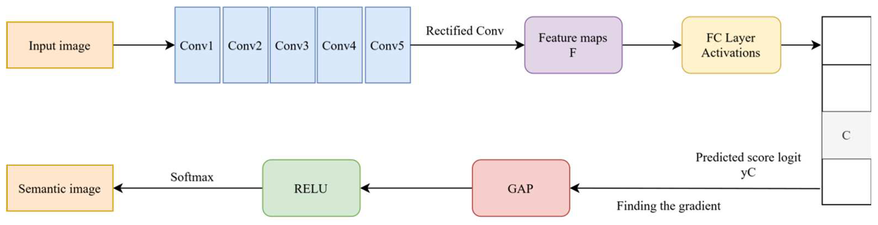
Figure 3.
Semantic importance map in Kodak.
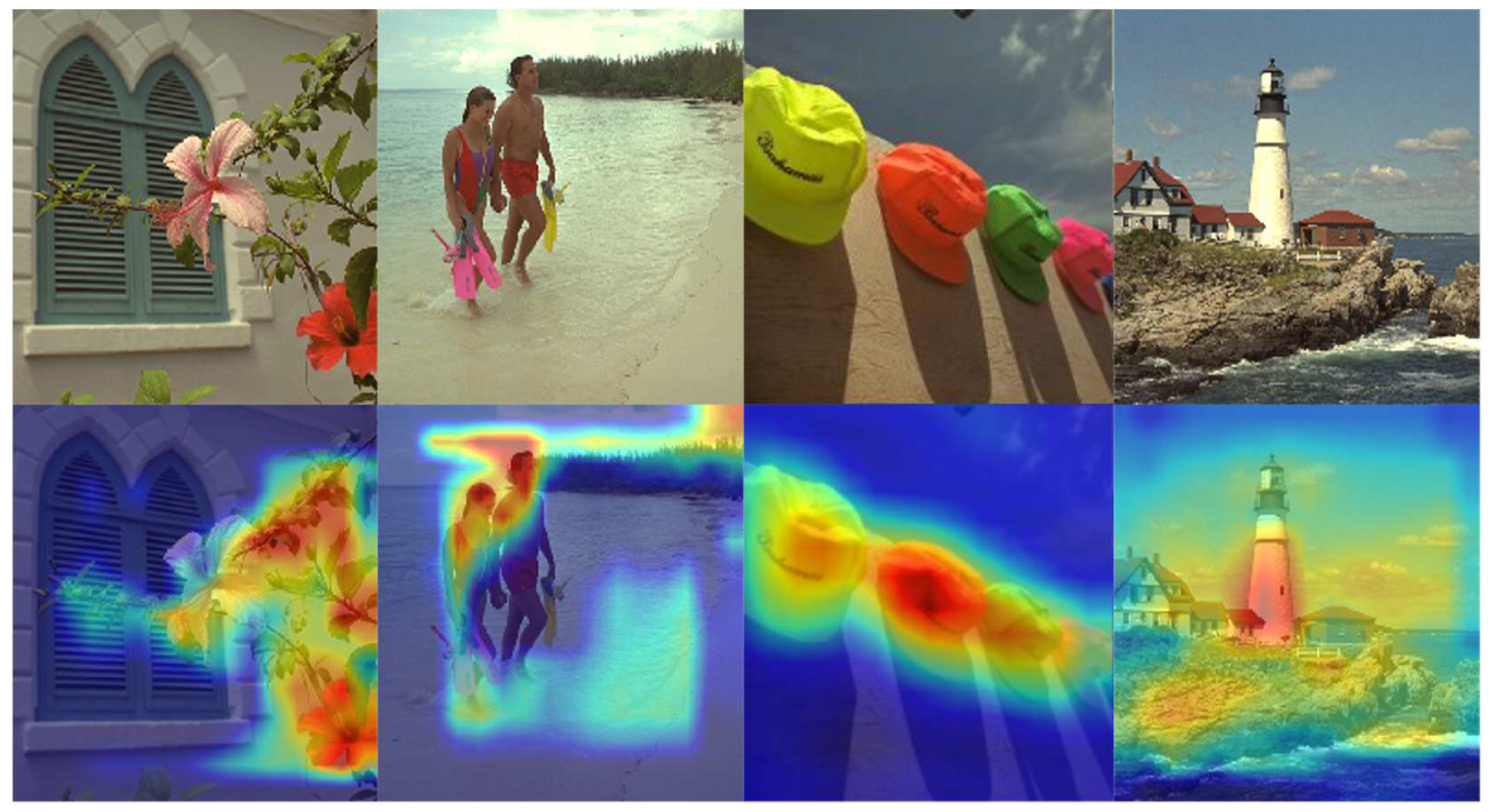
Figure 4.
Image compression network.
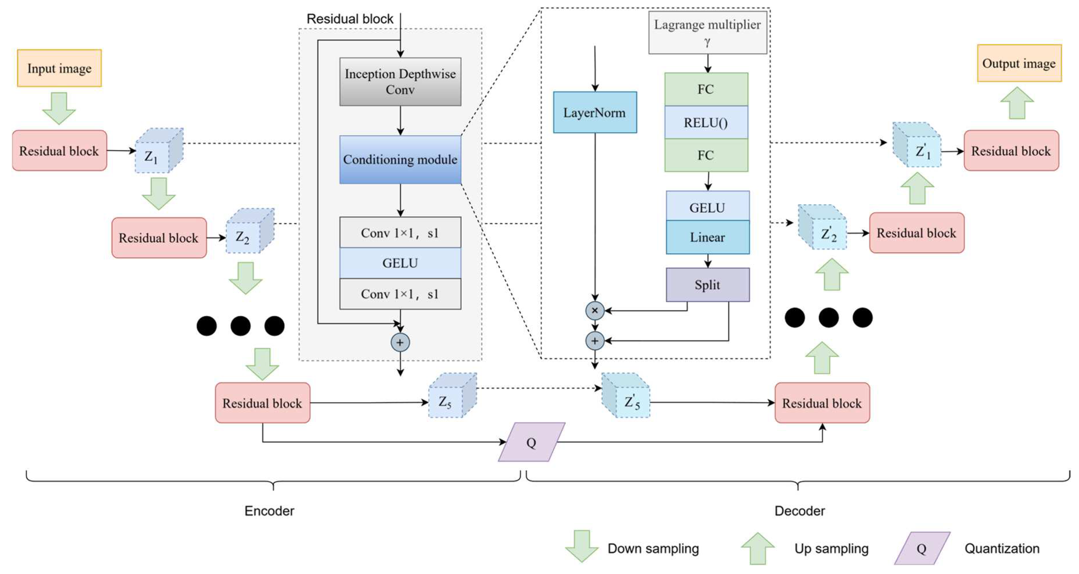
Figure 5.
Comparative experiments are conducted on the Kodak public dataset against JPEG, JPEG2000, BPG, TCM, and INN methods. (a) Displays the comparison results of PSNR; (b) Displays the comparison results of the MS-SSIM.
Figure 5.
Comparative experiments are conducted on the Kodak public dataset against JPEG, JPEG2000, BPG, TCM, and INN methods. (a) Displays the comparison results of PSNR; (b) Displays the comparison results of the MS-SSIM.
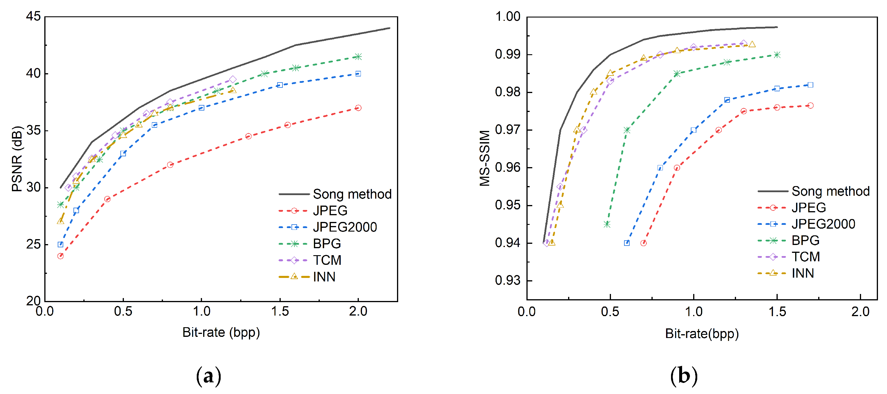
Figure 6.
Comparative experiments are conducted on the CLIC 2022 public dataset against JPEG, JPEG2000, BPG, TCM, and INN methods. (a) Displays the comparison results of PSNR; (b) Displays the comparison results of the MS-SSIM.
Figure 6.
Comparative experiments are conducted on the CLIC 2022 public dataset against JPEG, JPEG2000, BPG, TCM, and INN methods. (a) Displays the comparison results of PSNR; (b) Displays the comparison results of the MS-SSIM.
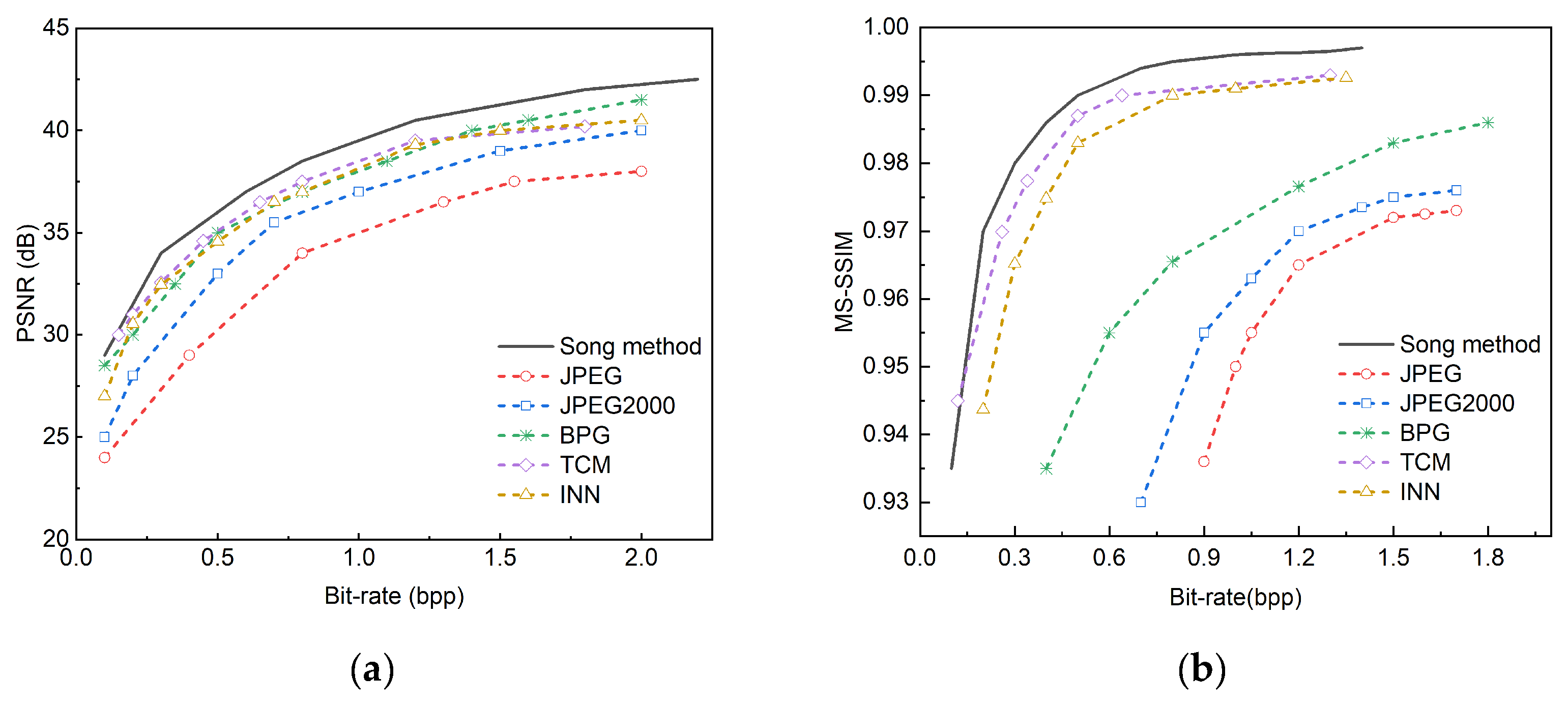
Figure 7.
Comparative experiments are conducted on the Tecnick TESTIMAGES public dataset against JPEG, JPEG2000, BPG, TCM, and INN methods. (a) Displays the comparison results of PSNR; (b) Displays the comparison results of the MS-SSIM.
Figure 7.
Comparative experiments are conducted on the Tecnick TESTIMAGES public dataset against JPEG, JPEG2000, BPG, TCM, and INN methods. (a) Displays the comparison results of PSNR; (b) Displays the comparison results of the MS-SSIM.
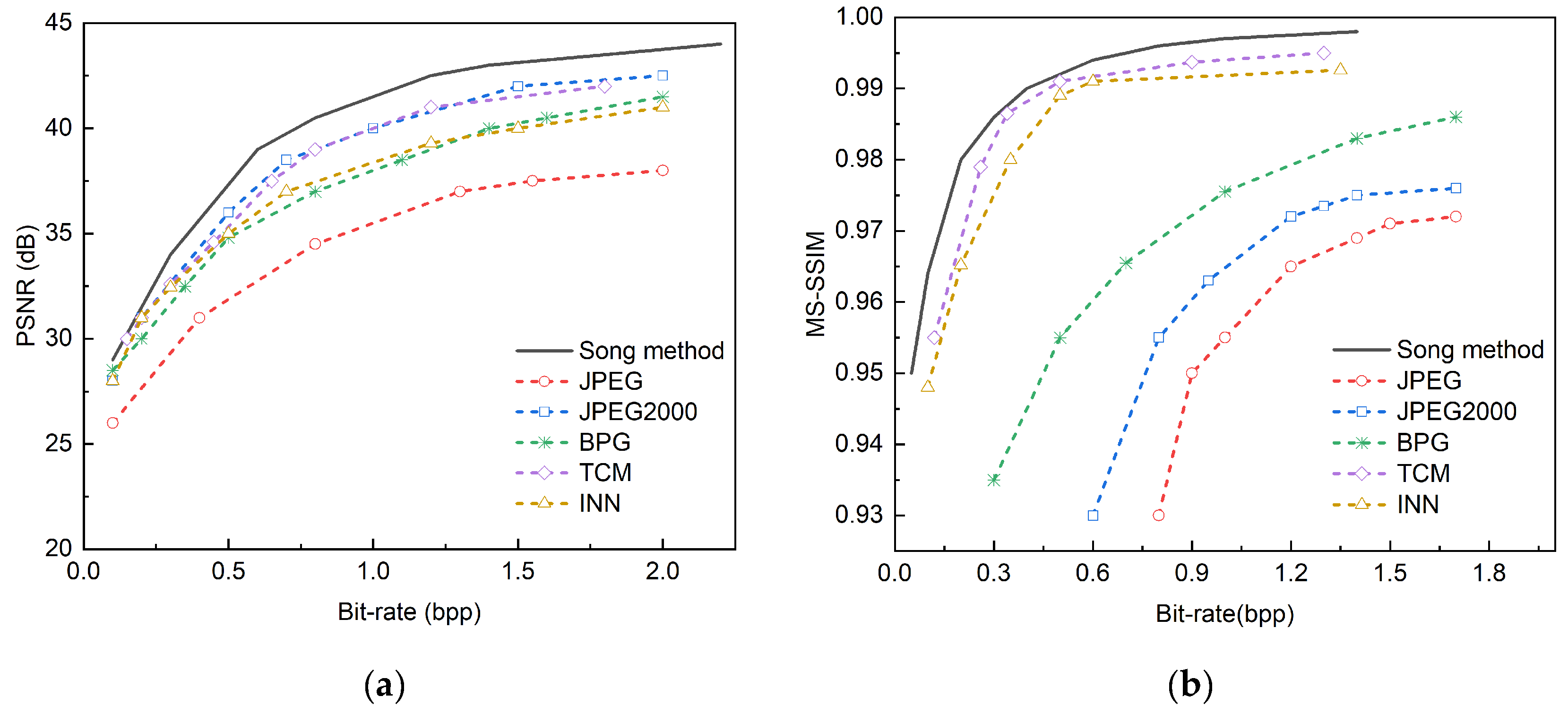
Figure 8.
Comparative experiments are conducted on the Kodak public dataset against DSSLIC , EDMS, DeepSIC and ADAPTIVE DIC methods. (a) Displays the comparison results of PSNR; (b) Displays the comparison results of the MS-SSIM.
Figure 8.
Comparative experiments are conducted on the Kodak public dataset against DSSLIC , EDMS, DeepSIC and ADAPTIVE DIC methods. (a) Displays the comparison results of PSNR; (b) Displays the comparison results of the MS-SSIM.
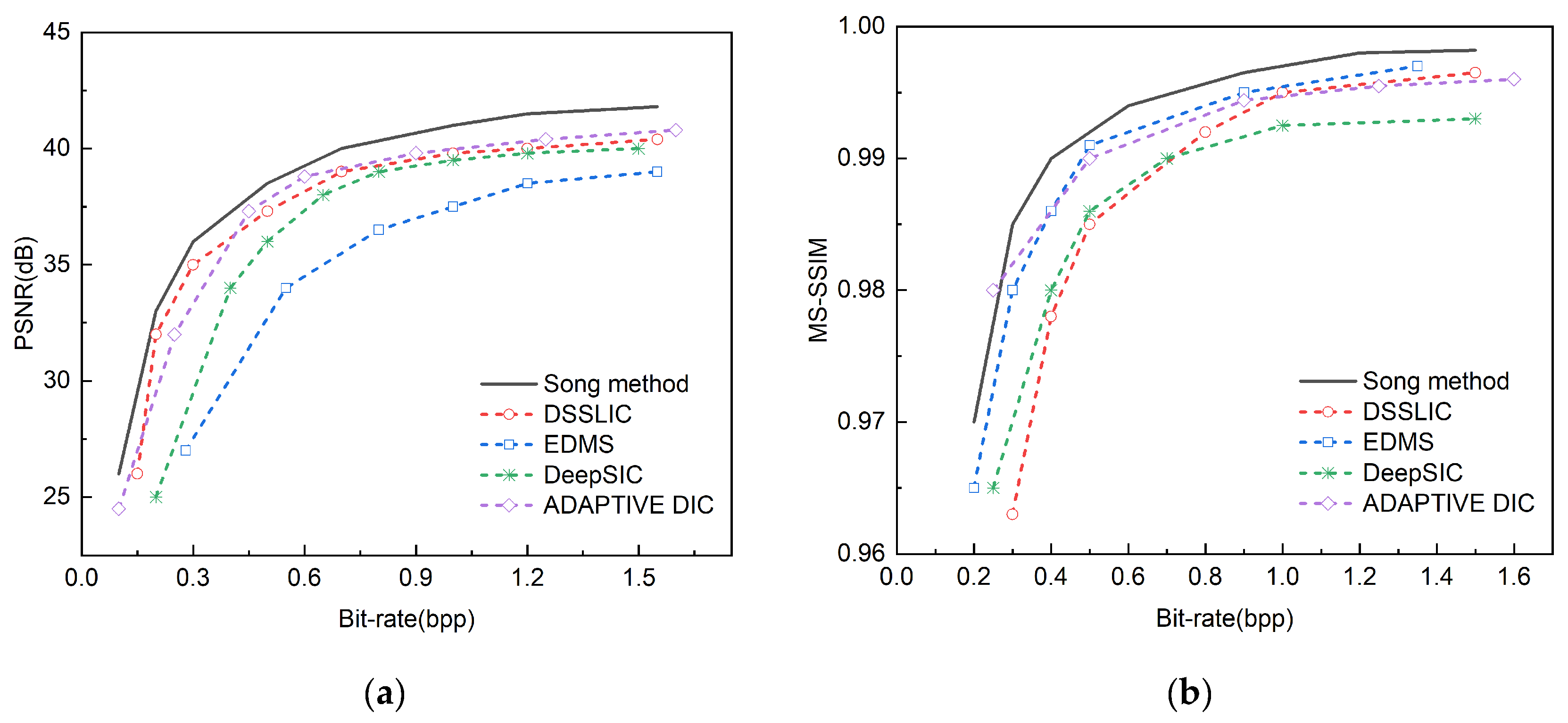
Figure 9.
Comparative experiments are conducted on the CLIC 2022 public dataset against DSSLIC, EDMS, DeepSIC and ADAPPTIVE DIC methods. (a) Displays the comparison results of PSNR; (b) Displays the comparison results of the MS-SSIM.
Figure 9.
Comparative experiments are conducted on the CLIC 2022 public dataset against DSSLIC, EDMS, DeepSIC and ADAPPTIVE DIC methods. (a) Displays the comparison results of PSNR; (b) Displays the comparison results of the MS-SSIM.
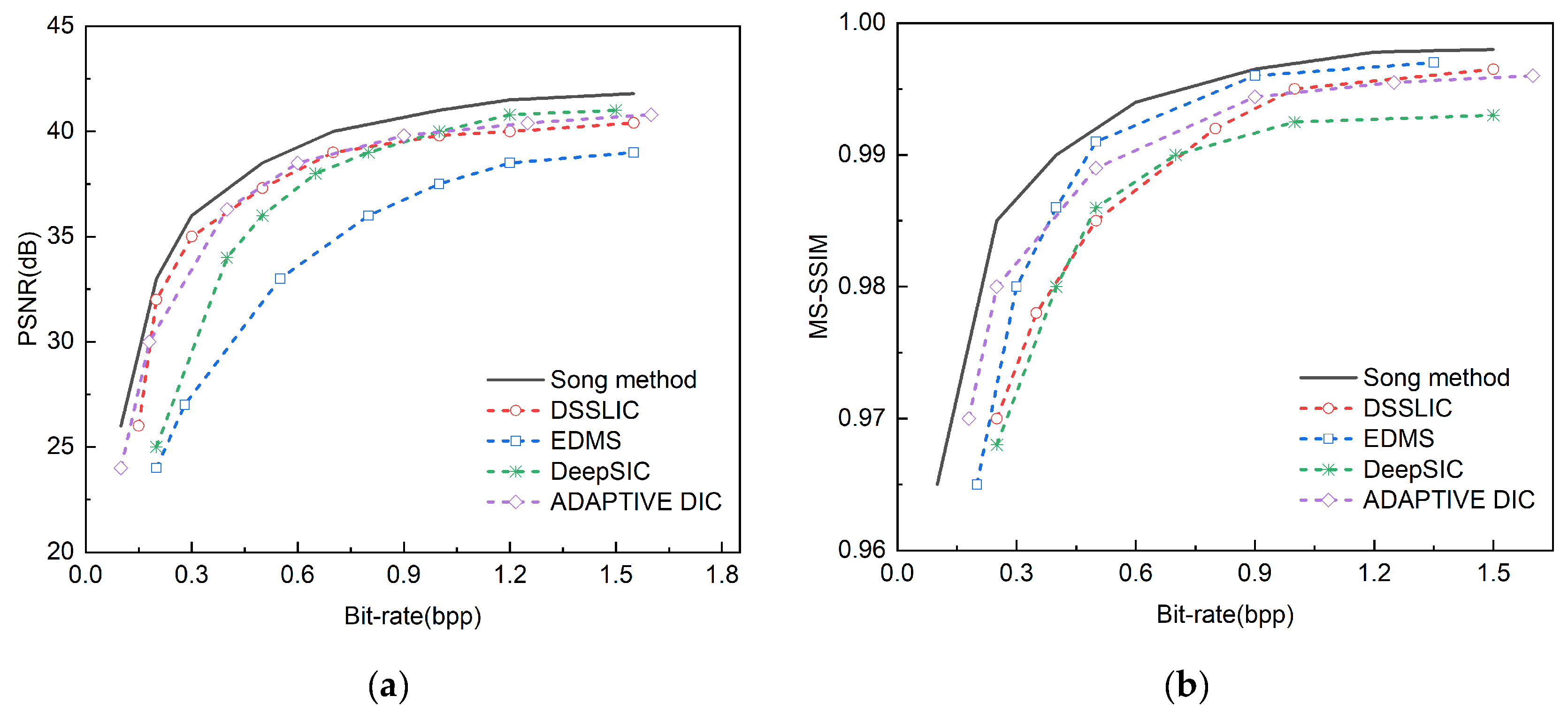
Figure 10.
Comparative experiments are conducted on the Tecnick TESTIMAGES public dataset against DSSLIC, EDMS , DeepSIC and ADAPTIVE DIC methods. (a) Displays the comparison results of PSNR; (b) Displays the comparison results of the MS-SSIM.
Figure 10.
Comparative experiments are conducted on the Tecnick TESTIMAGES public dataset against DSSLIC, EDMS , DeepSIC and ADAPTIVE DIC methods. (a) Displays the comparison results of PSNR; (b) Displays the comparison results of the MS-SSIM.
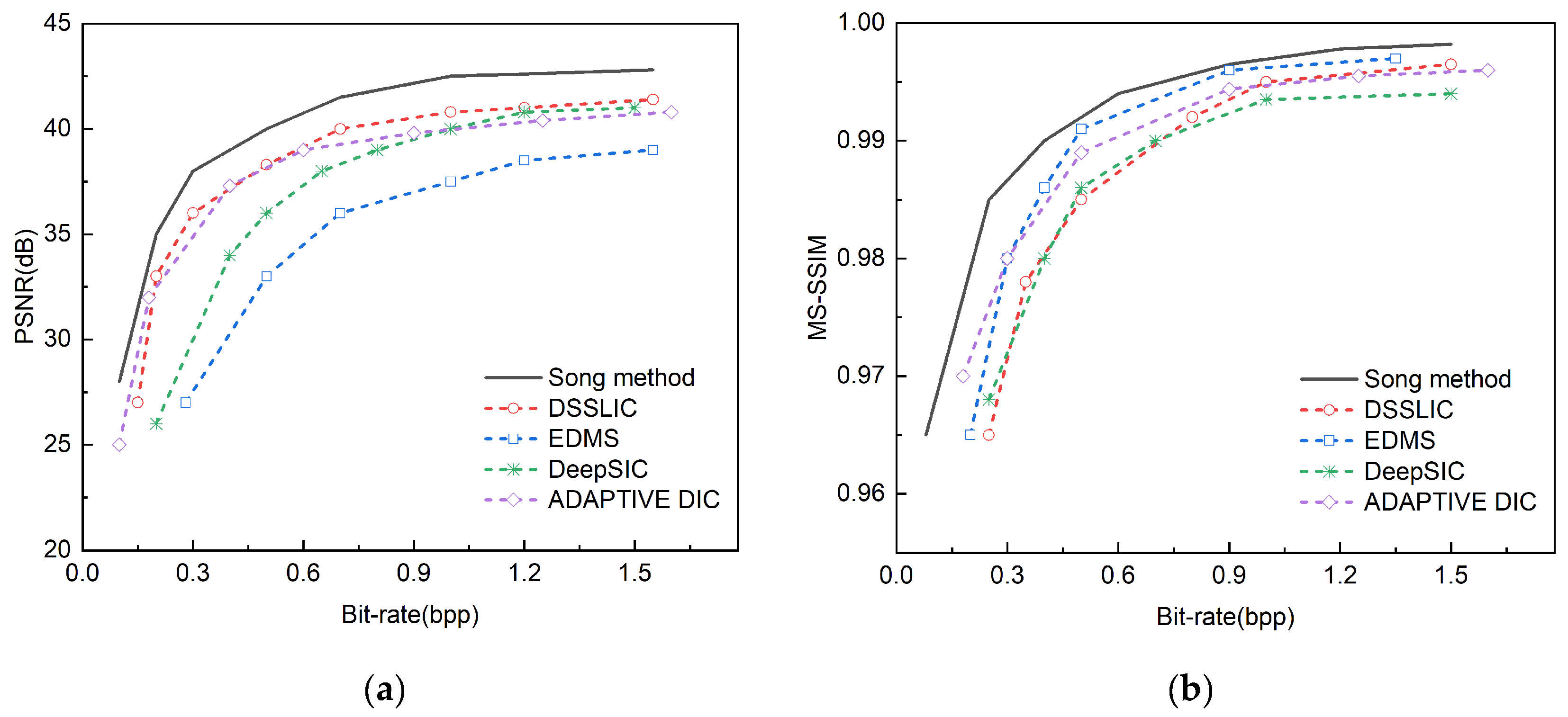
Figure 11.
Comparative experiments are conducted on the CLIC 2022 public dataset against MAE, Coarse-to-Fine, ELIC and QVRF methods. (a) Displays the comparison results of PSNR; (b) Displays the comparison results of the MS-SSIM.
Figure 11.
Comparative experiments are conducted on the CLIC 2022 public dataset against MAE, Coarse-to-Fine, ELIC and QVRF methods. (a) Displays the comparison results of PSNR; (b) Displays the comparison results of the MS-SSIM.
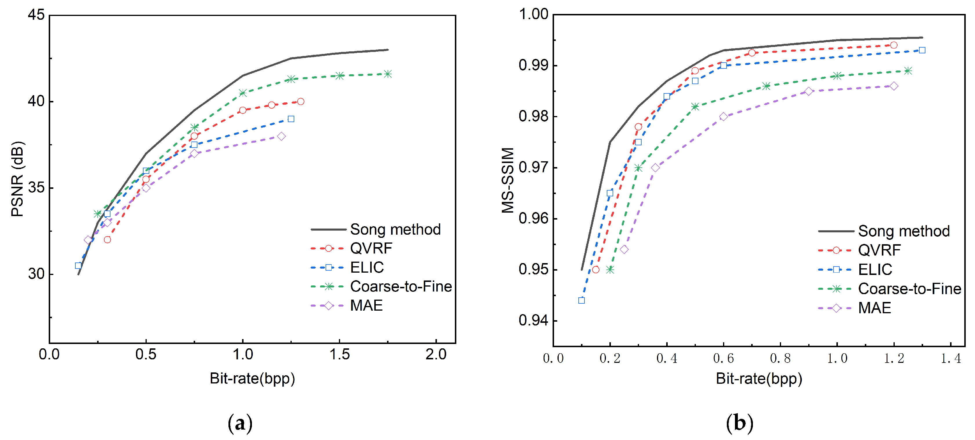
Figure 12.
Comparative experiments are conducted on the Tecnick TESTIMAGES public dataset against MAE , Coarse-to-Fine , ELIC and QVRF methods. (a) Displays the comparison results of PSNR; (b) Displays the comparison results of the MS-SSIM.
Figure 12.
Comparative experiments are conducted on the Tecnick TESTIMAGES public dataset against MAE , Coarse-to-Fine , ELIC and QVRF methods. (a) Displays the comparison results of PSNR; (b) Displays the comparison results of the MS-SSIM.
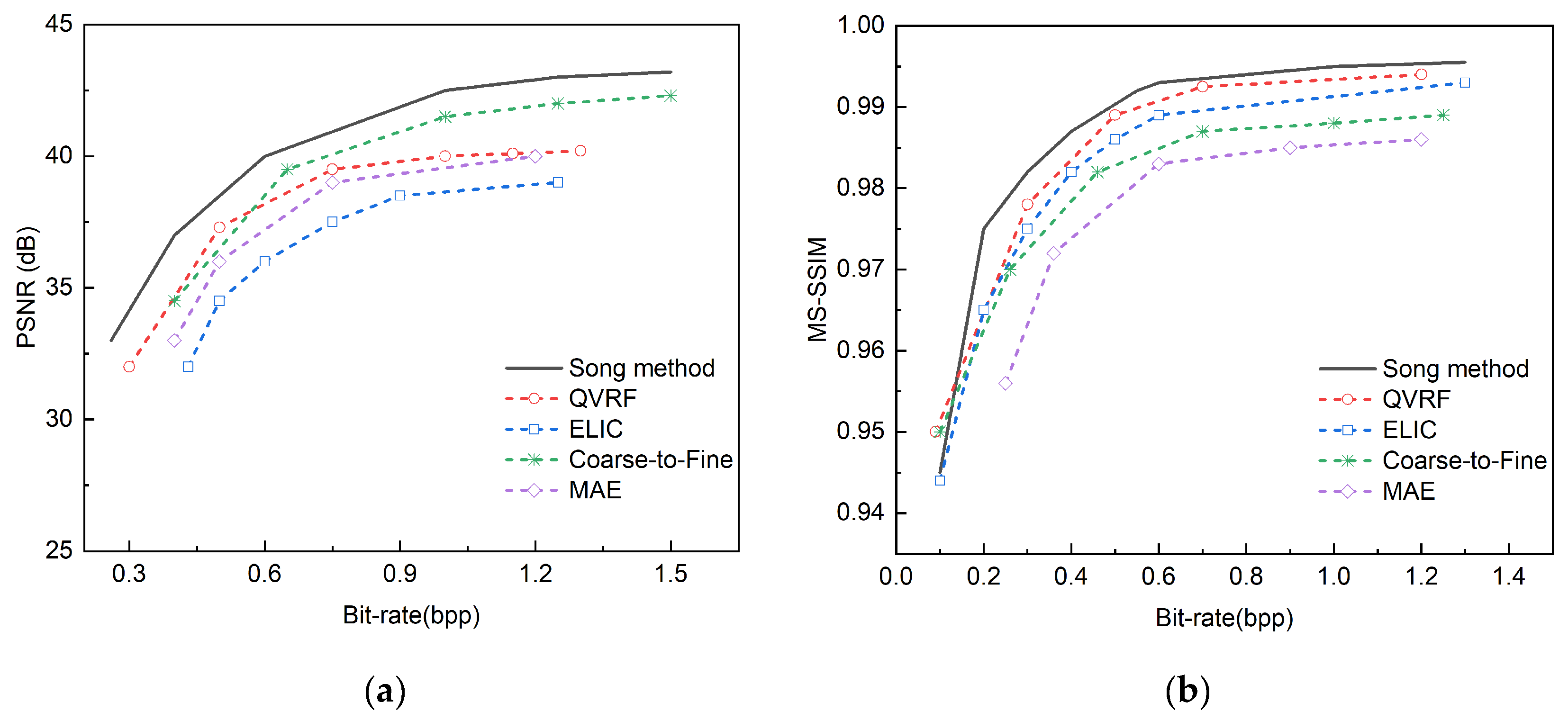
Figure 13.
Comparison of decompressed images at the same bit rate. From left to right are the original image, JPEG, JPEG2000, BPG, and the overall visual image comparison after decompression using the method in this paper.
Figure 13.
Comparison of decompressed images at the same bit rate. From left to right are the original image, JPEG, JPEG2000, BPG, and the overall visual image comparison after decompression using the method in this paper.
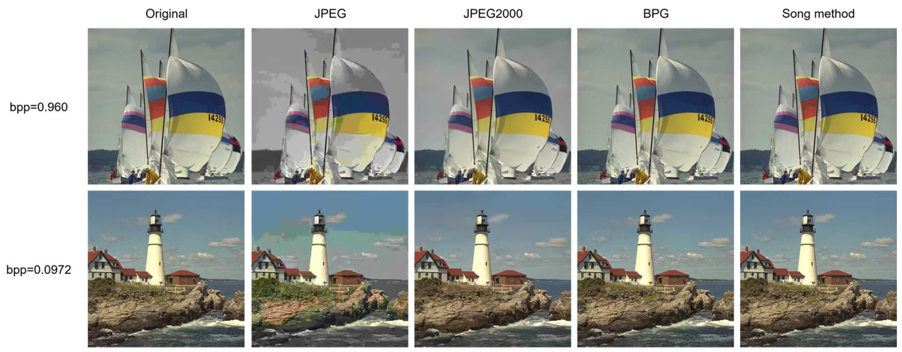
Figure 14.
Comparison of MS-SSIM under different bpp. The image in the upper right corner of each figure is the magnified effect of the important area of the image in the red frame. It is recommended to zoom in for observation.
Figure 14.
Comparison of MS-SSIM under different bpp. The image in the upper right corner of each figure is the magnified effect of the important area of the image in the red frame. It is recommended to zoom in for observation.
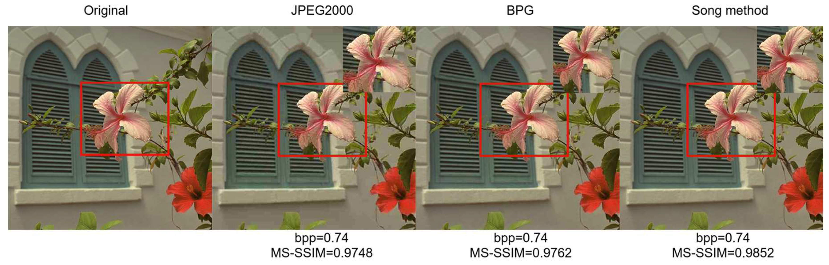
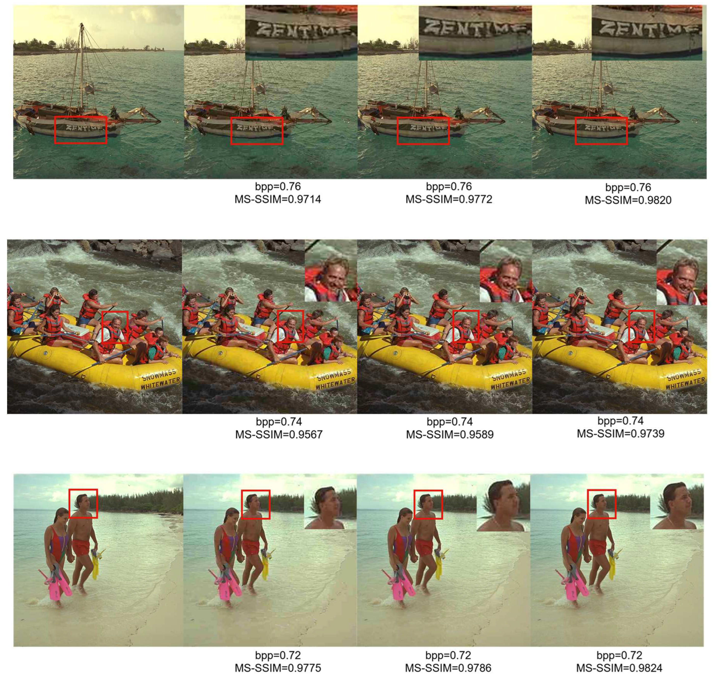
Figure 15.
Comparison of variable rate module ablation experiments on the Kodak dataset.
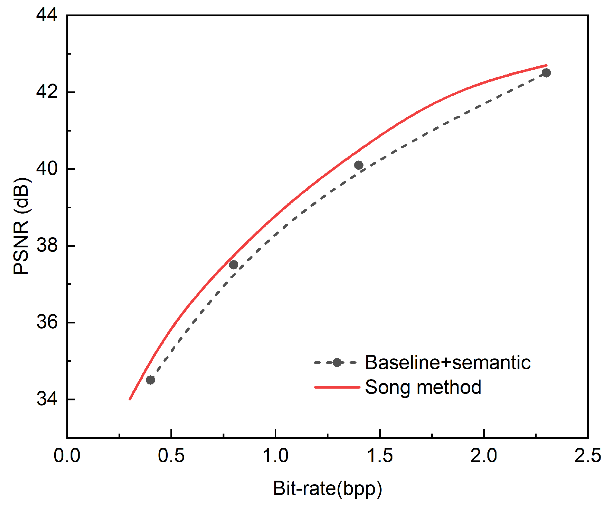

Table 1.
Comparison of indicators on the Kodak dataset when the bit rate is 1.12.
| Literature date | Bibliography | Module | PSNR | MS-SSIM |
|---|---|---|---|---|
| 1991 | [1] | JPEG | 33.2 | 0.950 |
| 2002 | [2] | JPEG2000 | 37.5 | 0.960 |
| 2017 | [3] | BPG | 38.5 | 0.973 |
| 2023 | [29] | TCM | 39.5 | 0.994 |
| 2021 | [30] | INN | 38.2 | 0.992 |
| Song method | 40.1 | 0.998 |
Table 2.
Comparison of indicators on the Kodak dataset when the bit rate is 0.75.
| Literature date | Bibliography | Module | PSNR | MS-SSIM |
|---|---|---|---|---|
| 2019 | [18] | DSSLIC | 39.8 | 0.991 |
| 2021 | [31] | EDMS | 34.2 | 0.993 |
| 2018 | [32] | DeepSIC | 37.3 | 0.985 |
| 2023 | [33] | ADAPTIVE DIC | 39.7 | 0.992 |
| Song method | 40.1 | 0.996 |
Table 3.
Comparison of indicators on the Kodak dataset when the bit rate is 1.25.
| Literature date | Bibliography | Module | PSNR | MS-SSIM |
|---|---|---|---|---|
| 2020 | [9] | MAE | 38 | 0.985 |
| 2021 | [10] | Coarse-to-Fine | 41.2 | 0.987 |
| 2022 | [11] | ELIC | 38.8 | 0.993 |
| 2023 | [12] | QVRF | 39.8 | 0.995 |
| Song method | 41.5 | 0.997 |
Table 4.
Data on ablation experiments. Bold font indicates optimal performance.
| Dataset | bpp | Metrics | Baseline | Baseline+semantic |
|---|---|---|---|---|
| Kodak | 1.124 | PSNR | 40.34 | 40.57 |
| MS-SSIM | 0.995 | 0.998 | ||
| Tecnick TESTIMAGES | 0.846 | PSNR | 40.40 | 40.42 |
| MS-SSIM | 0.993 | 0.996 | ||
| CLIC 2022 | 0.836 | PSNR | 39.42 | 39.41 |
| MS-SSIM | 0.992 | 0.994 |
Disclaimer/Publisher’s Note: The statements, opinions and data contained in all publications are solely those of the individual author(s) and contributor(s) and not of MDPI and/or the editor(s). MDPI and/or the editor(s) disclaim responsibility for any injury to people or property resulting from any ideas, methods, instructions or products referred to in the content. |
© 2025 by the authors. Licensee MDPI, Basel, Switzerland. This article is an open access article distributed under the terms and conditions of the Creative Commons Attribution (CC BY) license (https://creativecommons.org/licenses/by/4.0/).
Copyright: This open access article is published under a Creative Commons CC BY 4.0 license, which permit the free download, distribution, and reuse, provided that the author and preprint are cited in any reuse.


