

Submitted:
18 November 2024
Posted:
19 November 2024
You are already at the latest version
Abstract
This paper presents a method for preserving the quality of video compressed with video codecs. The video codecs used in this article are H.264/AVC (Advanced Video Coding) and its successor H.265/HEVC (High Efficiency Video Coding). The aim of the article is to present a method for enhancing the video quality for high compression values by preprocessing video frames using Deep Neural Network (DNN). The proposed method reduces the degree of image quality degradation caused by lossy video compression by improving the detail quality of the output video frames after decompression. The proposed method improves video quality for high QP (Quantization Parameter) values beginning from 25 and above. Compared to the popular trend of improving the video quality of already degraded video, the presented method attempts to improve the quality by modifying the image before the compression process by the video codec. The image is modified by DNN to obtain the lowest possible loss of video quality, represented by quality coefficients, but above all by the visual reception of the video by the viewer, enabling increased perception of more details in conditions of high video compression.
Keywords:
AVC
; H.264
; HEVC
; H.265
; video quality
; enhancement
; improvement
; preservation
1. Introduction
Nowadays, the demanded amount of memory needed to store data is an important issue in the field of Information Technology. One of the methods to solve this problem is the use of lossless and lossy compression. Video codecs are specialized data compression for video purposes. Lossless compression is characterized by a large amount of memory needed to store data. On the other hand lossy compression allows to store video data in a form that is imperceptibly changed or slightly noticeable to the human eye by maintaining the appropriate degree of video compression, while offering a reduction in the need to store video on data carriers with limited storage capacity. Examples of popular video codecs that offer both lossless and lossy compression are: H.264, H.265 and AV1. With the advent of lossy video compression, the natural course of things was a need to recover previously lost video quality which was compressed in order to reduce the amount of memory needed to store it.
The purpose of this publication is to present the developed method that enables improving the quality of compressed video by applying the process of enhancing image characteristics before compression rather than after decompression, which is commonly used in most methods. The problem of improving image quality after use of compression codec is challenging and complexity of it increases with the greater levels of compression (QP coefficient), which, at its highest values, makes it difficult to correctly recognize the details of objects or generally makes them less visible in the image. The presented method is based on the use of DNN to preprocess the image, which will be subjected to AVC and HEVC compression to increase the similarity of the compressed image to the original image.
The structure of the manuscript is as follows: The literature related to this publication is presented at the beginning. Next, the idea of the proposed method will be presented and the Artificial Neural Network (ANN) learning method will be discussed. Subsequently, the results of the method will be presented and discussed. The final part of the manuscript contains a summary of the research results and suggestions for further development. Appendix A shows preview of video compression comparison with the use of the proposed method and without it.
2. Related Work
In reviewing the literature related to video quality improvement, attention should be paid to the following issues: video enhancement [1,2,3,4,5,6], video restoration [7,8,9], video deblurring [10,11,12], video denoising [13,14,15,16], video dehazing [17,18] and video super-resolution [19,20,21]. The above-mentioned issues overlap and share and have a common feature of improving video quality.
The Video Super-Resolution methods are designed to improve video quality by increasing image resolution while maintaining image quality. The Video Deblurring and Video Denoising methods are designed to improve video quality by removing unwanted graphic effects. The Video Restoration and Video Enhancement methods, on the other hand, are intended to improve the overall video quality.
There are two main trends in the available literature on restoring video quality. The first one is based on the use of a sequence of video frames [7,8,9,10,11,22,23,24]. The second one is based on the principle of improving a single video frame [25,26,27,28].
Many of the methods available in the literature perform video quality restoration through methods based on the processing of a single video frame [26,27,28,29]. The use of this type of methods enables the parallelization of calculations.
Methods using a sequence of video frames can be divided into: sliding-window-based [7,8,9,10,11,23,24,25] and recurrent [30,31,32,33,34,35,36,37] methods. Sliding window-based methods in general use multiple input frames to generate a single improved video frame. Methods based on recursion utilize recurrence for their computations and require more time than sliding window-based methods.
Among the methods aimed at improving the quality of compressed video, there are methods that can be applied to various types of compression [3,5] and as well as dedicated methods to a given type of video codec [2,3,4,23,38].
An important aspect of this work is the fact that the focus is mainly on improving the quality of compressed video frames after passing through a process of compression using the H.264 and H.265 codec. Therefore, learning of the features of the HEVC codec as best as possible is crucial for proposed neural network. A good step is to analyze the architecture of the neuron-based networks used in conjunction with the encoding of the HEVC codec. Without trying to obtain the characteristics of the HEVC codec through simulation/reconstruction of its actions or methods such as deep reinforcement learning [39] or black box gradient estimation [40,41,42,43,44], a problem known as no continuity in the gradient can be encountered (non-differentiability of certain processing block), which destabilizes the training process or makes it impossible.
In the case of processing video using the HEVC codec, deep neural networks are used to replace encoding HEVC through end-to-end systems completely based on processing video by subsequent blocks of neural network. In case of [45] authors replaced processing blocks of HEVC algorithm by corresponding to them DNN blocks. Transform and Inverse transform blocks were replaced by Residual Encoder/Decoder Net, Motion Compensation block was replaced by Motion Compensation Net+MV Encoder/Decoder Net+Optical Flow Net, and Entropy Coding block was replaced by Bit Rate Estimation Net [45]. Another approach similar to [45] presented in work [46] (MOVI-Codec) is to use LSTM-Unet neural network which allow to skip Motion Compensation block in process of compression video. Another possibility for applying DNN is improving the speed of encoding HEVC by reducing complexity of some of HEVC algorithms. The papers [47,48] (IPCNN, ImageNet) shows that by replacing algorithms for intra prediction mode decision by a Convolutional Neural Networks (CNNs) it possible to have less computational complexity but similar or better performance. Some methods aim to improve certain stages of HEVC processing, like in work [49] where researchers by using DNN models like DAIN [50] and SloMo [51] improve effectiveness of codec in interpolating frames. In the work of Çetinkaya et al. [52] the use of CNNs for Coding Tree Unit process can be also seen.
To measure quality of processed frames/images by compression methods, image quality assessment (IQA) metrics like Peak Signal-to-Noise Ratio (PSNR) and Structural Similarity Index Measure (SSIM), Visual Information Fidelity (VIF), Mean Square Error (MSE), Mean Opinion Score (MOS), BD-PSNR and BD-Rate are used.
PSNR provides an indication of the overall quality of an image, but it does not take into account human perception [53,54,55]. SSIM takes into account both the luminance and chrominance channels of an image, making it a more robust measure than PSNR alone [53,55,56]. Visual Information Fidelity (VIF) measures how well a compression algorithm preserves the visual information in an image. VIF is used extensively in video coding standards such as H.264 and H.265, where it is combined with other metrics to optimize image quality [53,55,56,57]. BD-PSNR and BD-Rate are measures of compression efficiency over a range of bitrate or quality values [58,59].
Mean Squared Error (MSE) refers to the average squared difference between two sets of data points or images. In the context of image quality assessment, it is a widely used metric that measures how closely the compressed image resembles its original counterpart. The lower the MSE value, the better the compression and the higher the perceived image quality. Mean Opinion Score (MOS) is a widely-used metric for evaluating the perceived quality of images, videos and other multimedia content by human perception. MOS is particularly useful for evaluating the effectiveness of image compression algorithms that aim to preserve visual quality while minimizing file size.
To evaluate efficiency of proposed in this paper method, metrics like PSNR and SSIM were calculated for the test video.
3. Concept of the Proposed Method
3.1. General Concept of the Proposed Method
The general idea of the proposed method of improving video quality is presented below in form of flowchart diagram (Figure 1). The elements of diagram are representing the subsequent steps taken to improve quality of compressed video frames.
In the proposed method the main component is the Adjusting DNN (ADNN). ADNN input is fed with a video frame which is to be subjected to AVC or HEVC compression. As a result of the operation of the neural network, subsequent frames are created which are video components assumed to have better visual quality compared to video subjected to AVC or HEVC compression without prior preparation with use of ADNN. ADNN input layer accepts a single frame of video image and returns a single frame (adjusted to HEVC codec) in the output.
Due to the characteristics of HEVC, it should be noted that ADNN works on the YUV444p colour model. In addition, due to hardware limitations, the presented neural network works natively with an image resolution of 128 × 128. Native work on the presented resolution for higher image resolutions is solved by using the Sliding window algorithm.
3.2. HEVC Compression Adjustment Learning Process
In order to present the learning process, the following objective function relationships will be discussed:
where is the mean square error; is the floor function; is the image obtained after HEVC compression; (Quantization Parameter) is the parameter determining the degree of HEVC compression; is the image created by the trained ADNN mimicking the image after HEVC compression; is the mean square error of the image produced by the ADNN in relation to the image compressed with HEVC, both parameterized by the value; is the ADNN error; is the tensor of the ADNN model weights; is the gradient of the ADNN objective function.
In the equations for and there are multiplication and division operations by the numerical value 255, respectively, this is due to the fact that the neural network performs better when input data is normalized (scaled) in the range . After all the computations are done on the processed frame to convert output of neural network to image form the output is multiplied by the value of 255 and then subjected to the function as each pixel value is represented in the form of integer values in the range .
The learning process of neural network consisted of 300 epochs of the learning algorithm. In this process, the Adam Optimizer algorithm was used. During learning process the learning rate value was changed to improve and speed up achieving convergence by neural network for a given problem. For the first 100 epochs, the learning rate value was set to 10−4. Then, the ANN giving the best results from 100 learning epochs was selected and for this ANN in the next 200 epochs, the learning rate was set 10−6. The batch size used was 16.
The training set consisted of 4,000 random images for each epoch from ImageNet dataset [60], which were transformed to a resolution of 128 × 128, then these images were subjected to HEVC compression with a value of 0. The training set prepared in this way was used in the learning process, which is equivalent to the entry in equation number 1. On the other hand, the entry in the same equation is equivalent to processing the image from the training set by performing the appropriate HEVC compression on the image, the degree of which is parameterized by the QP value in the range of integer values .
Considering the similarities in image processing by H.264/AVC (Advanced Video Coding) and its successor H.265/HEVC (High Efficiency Video Coding) video codecs, only one DNN was trained on the HEVC characteristics.
3.3. Neural Network Architecture
The ADNN structure presented in this manuscript uses layers such as: BatchNormalization, Concatenate, Conv2D, Conv2DTranspose, DepthwiseConv2D and multiplication operation. The activation functions used in the ADNN structure are GELU and LeakyReLU.
Table 1, Table 2 and Table 3 show the ADNN structure. Table 1 and Table 2 show the Convolution Basic Layer (CBL) and Transposed Convolution Basic Layer (TCBL), respectively. The logical layers are composed of a sequence of the previously mentioned base layers offered by the TensorFlow machine learning library. Table 3 shows the general model of applied ANN. In Table 1, Table 2 and Table 3, individual numerical values in layer type descriptions refer to previous layer numbers.
Table 2 and Table 3 show that there is only one difference between the presented logical layers, which is the use of a different basic layer for the third layer in the sequential logical models.
In Table 3, the Input image value is the image stored in the range of numeric values to be subjected to ADNN processing. is the compression value from the range unified to the range of number values on which DNN operates in accordance with the following relationship:
where (Quantization Parameter) is the parameter determining the degree of HEVC compression; is the calculated value of converted for ANN computations purpose in the value range .
Parameters of ADNN relating to hardware requirements are shown in Table 4. Speed of ANN processing was measured on GeForce 1080Ti GTX 11GB graphics processing unit (GPU).
4. Results
In this section, the results of the described method will be presented and discussed. First AVC and then HEVC results of improving the quality of video compressed with video codec in the context of prior preparation of video frames by ADNN will be presented and discussed.
The research was conducted on a Linux operating system (Ubuntu 22.04) using the TensorFlow version 2.13.0 machine learning library. To process video the FFmpeg video handling library (version 4.4.2-0ubuntu0.22.04.1) was used. The source codes were written in Python version 3.10.12.
In the further part of the section, the performance results of presented method obtained for individual frames of the test video [61] and for selected DAVIS [62], GoPro [63], REDS [64], Vimeo-90K-T [65] test datasets of videos are presented. For DAVIS [62], the selected tested videos are: bear, blackswan, boat, bus and dog. For GoPro [63], the selected tested videos are: GOPRO0384, GOPRO0385, GOPRO0396, GOPRO0410. For REDS [64], the selected tested videos are: 001, 002, 003, 004 and 005. For Vimeo-90K-T [65], the selected tested videos are: 00001 and 00002. Video enhancement tests were conducted by default at 640 × 640 video resolution. Due to the fact that ADNN was trained for images with a resolution of 128 × 128, the moving window method was used to process the entire image.
The effectiveness of the method for selected values of QP are presented through coefficients (PSNR and SSIM) that mathematically determine the similarity between images. These coefficients represent the calculated similarity value however, it is not an absolute determinant of image quality. The potentially human-visible modification of the image as a result of the coefficient calculation may be considered insignificant. There is also a possibility of the reverse situation, consisting in finding an improvement in image quality by a human, while the calculation of the coefficient shows otherwise.
4.1. AVC Compression Enhancement Research Results
The results of ADNN processing in the context of improving the visual quality of video subjected to AVC compression are presented in Table 5, Table 6 and Table 7, which show the averaged results of processing on sample test video frames [61] with the image resolution changed to 640 × 640.
A graphical preview of ADNN processing in the context of improving video quality is shown in Figure 3, Figure 4, Figure 5, Figure 6, Figure 7 and Figure 8 and in Appendix A.
From the analysis of the results in Table 5, Table 6 and Table 7 and Figure 2, it is noticeable that there is no direct improvement and a slight deterioration of the PSNR value for ADNN compression in comparison to AVC compression. This is due to the fact that ADNN makes more changes to the image than native AVC compression.
Based on the results of the study, it was found that the proposed method works effectively when there is no direct translation of the QP compression factor value fed to the ADNN input to the target QP compression value for AVC compression. Starting from QP value 25 there is noticeable tendency to improve the quality of the video.
In order to properly present the use of ADNN capabilities, a conversion table (Table 8) was compiled on the basis of the conducted research, which presents suggested compression values for ADNN in relation to the target AVC compression value. It should be emphasized that conversion values in Table 8 are used further in this manuscript to present further results in the context of the AVC compression. Meaning that for a compression value, e.g. QP = 45, the value of the compression ratio at the ADNN input was given in accordance with conversion table (Table 8) as 36, and then processed image from ADNN was given for the AVC video codec, for which the value of compression is QP = 36. Thus, keeping for the indicated value a larger number details with a similar output file size.
In order to utilize the conversion table (Table 8), it is needed to first determine the target compression ratio QP for AVC, then read the corresponding QP value for ADNN from the table and use it in the calculations for the image preprocessing by ADNN. Using the values from the conversion table when determining the QP value for ADNN provides a greater visual quality improvement value for the AVC compression target QP value, than using directly.
The average gain of the proposed method in numerical form for specified QP value can be obtained by reading the values from Table 8. Average of ∇PSNR is 2.03 dB and the average value of file size reduction is 1.16 KB for QP value greater than 24. The graphical results of the ADNN processing are shown in Figure 3, Figure 4, Figure 5, Figure 6, Figure 7 and Figure 8.
Figure 3.
Preview of compression effects for frame 200 and 400 of the test video [61] with QP=41 (viewed from the top, the rows represent consecutive video frames, viewed from the left, the consecutive columns represent the original image, the image compressed by pure AVC, and the image processed by ADNN and compressed by AVC).
Figure 3.
Preview of compression effects for frame 200 and 400 of the test video [61] with QP=41 (viewed from the top, the rows represent consecutive video frames, viewed from the left, the consecutive columns represent the original image, the image compressed by pure AVC, and the image processed by ADNN and compressed by AVC).
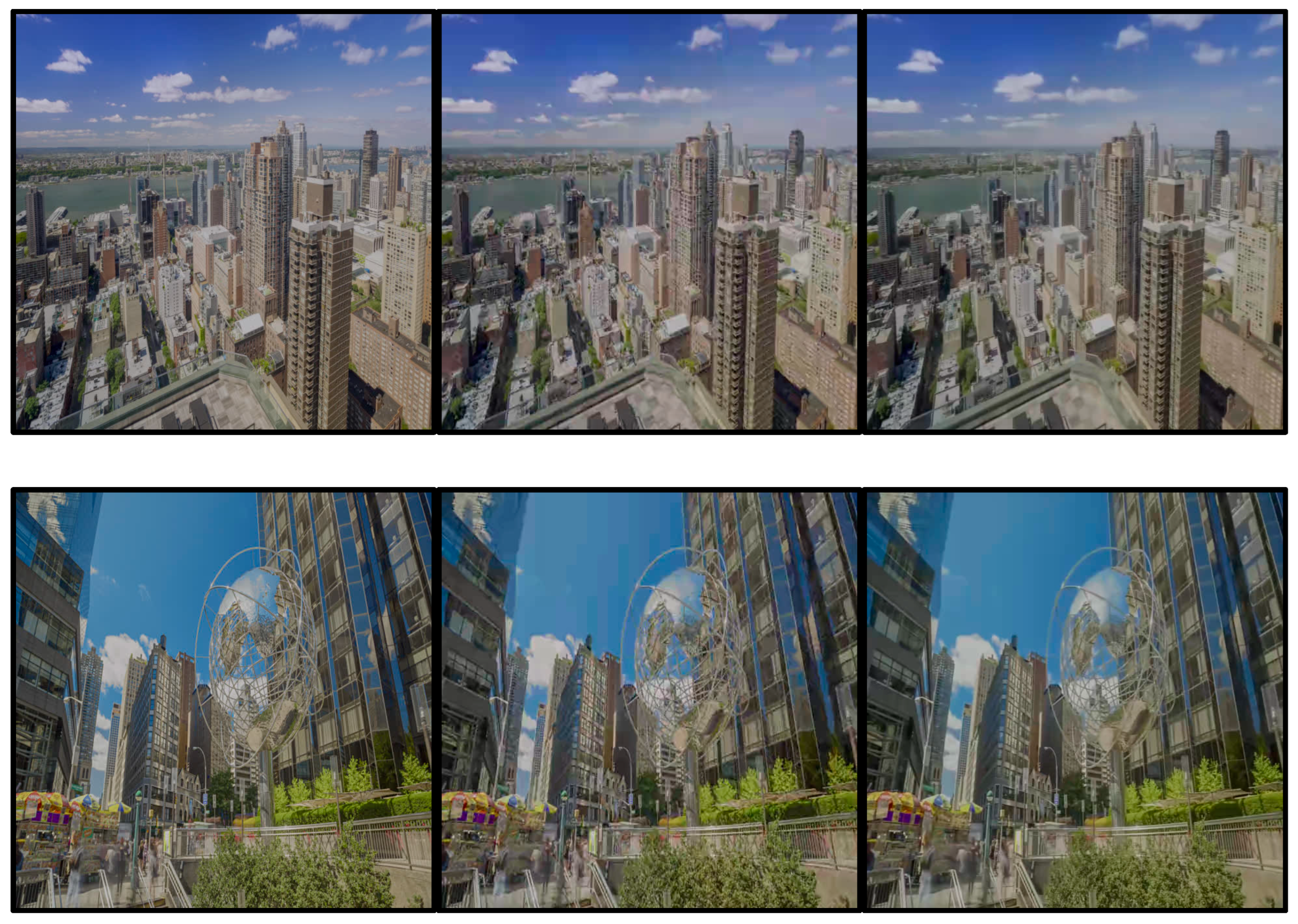
Figure 4.
Preview of compression effects for frame 600 and 800 of the test video [61] with QP=45 (viewed from the top, the rows represent consecutive video frames, viewed from the left, the consecutive columns represent the original image, the image compressed by pure AVC, and the image processed by ADNN and compressed by AVC).
Figure 4.
Preview of compression effects for frame 600 and 800 of the test video [61] with QP=45 (viewed from the top, the rows represent consecutive video frames, viewed from the left, the consecutive columns represent the original image, the image compressed by pure AVC, and the image processed by ADNN and compressed by AVC).
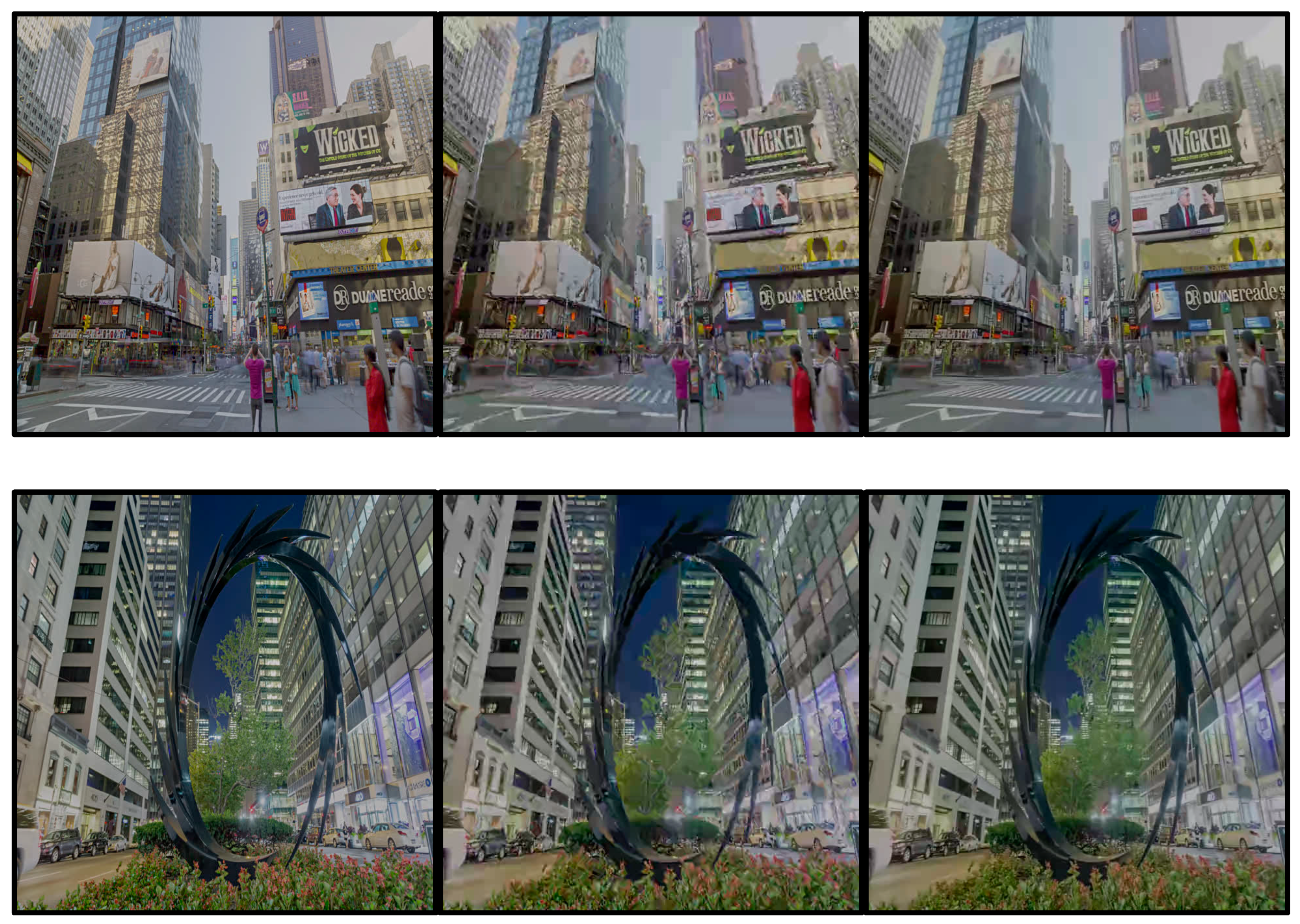
Figure 5.
Preview of compression effects for frame 600 and 800 of the test video [61] with QP=51 (viewed from the top, the rows represent consecutive video frames, viewed from the left, the consecutive columns represent the original image, the image compressed by pure AVC, and the image processed by ADNN and compressed by AVC).
Figure 5.
Preview of compression effects for frame 600 and 800 of the test video [61] with QP=51 (viewed from the top, the rows represent consecutive video frames, viewed from the left, the consecutive columns represent the original image, the image compressed by pure AVC, and the image processed by ADNN and compressed by AVC).
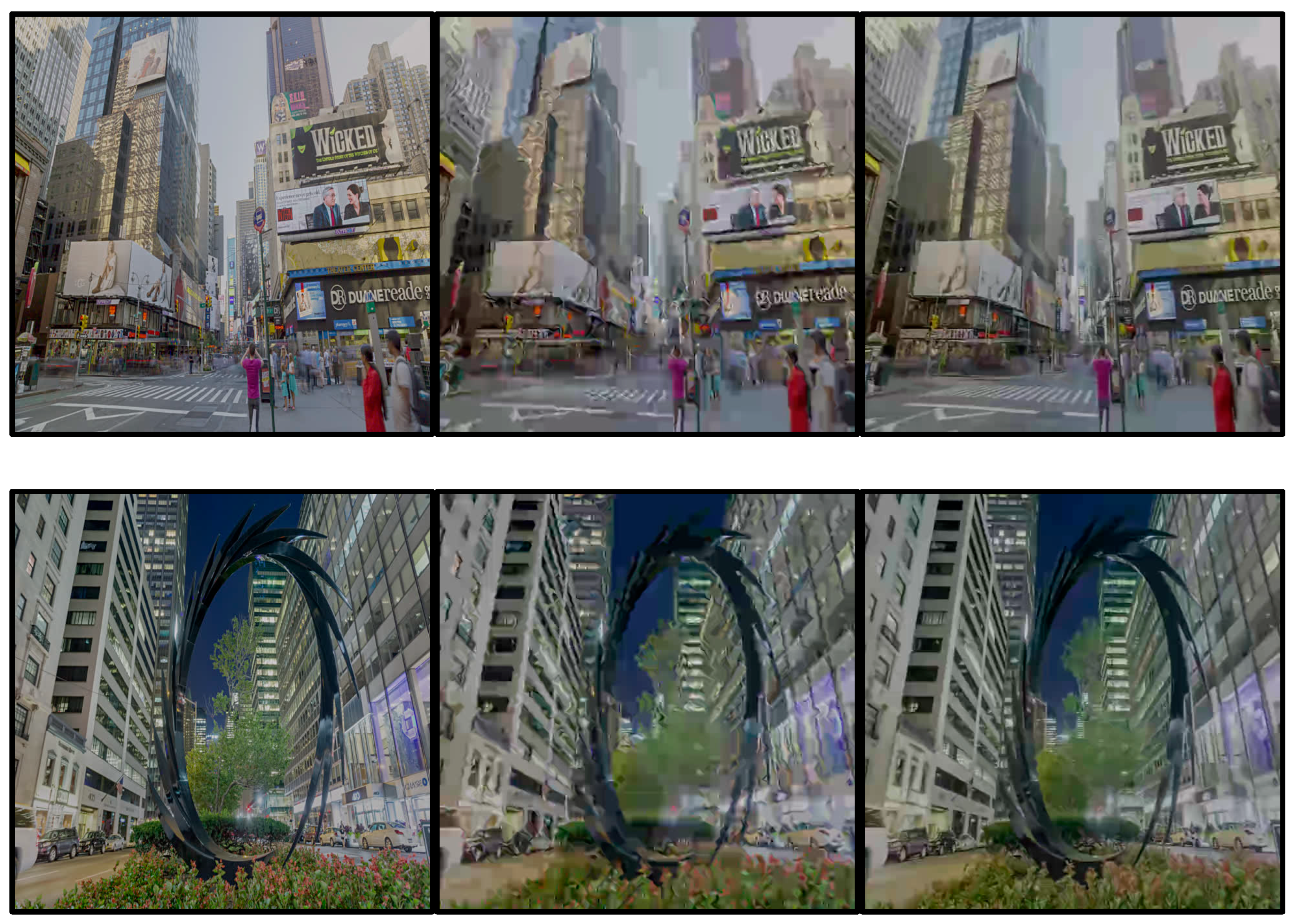
Figure 6.
Preview of compression effects for frame 200 with QP=43 of the test video [61] (viewed from the left: the image compressed by pure AVC, and the image processed by ADNN and compressed by AVC).
Figure 6.
Preview of compression effects for frame 200 with QP=43 of the test video [61] (viewed from the left: the image compressed by pure AVC, and the image processed by ADNN and compressed by AVC).
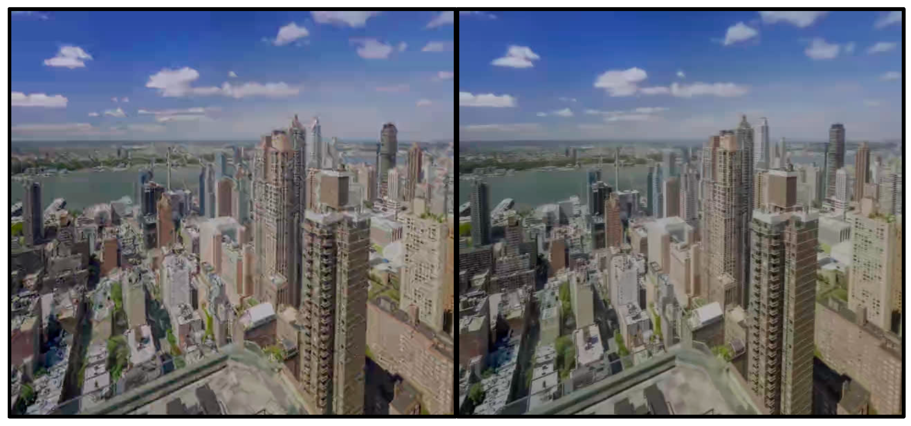
Figure 7.
Preview of compression effects for frame 600 with QP=47 of the test video [61] (viewed from the left: the image compressed by pure AVC, and the image processed by ADNN and compressed by AVC).
Figure 7.
Preview of compression effects for frame 600 with QP=47 of the test video [61] (viewed from the left: the image compressed by pure AVC, and the image processed by ADNN and compressed by AVC).
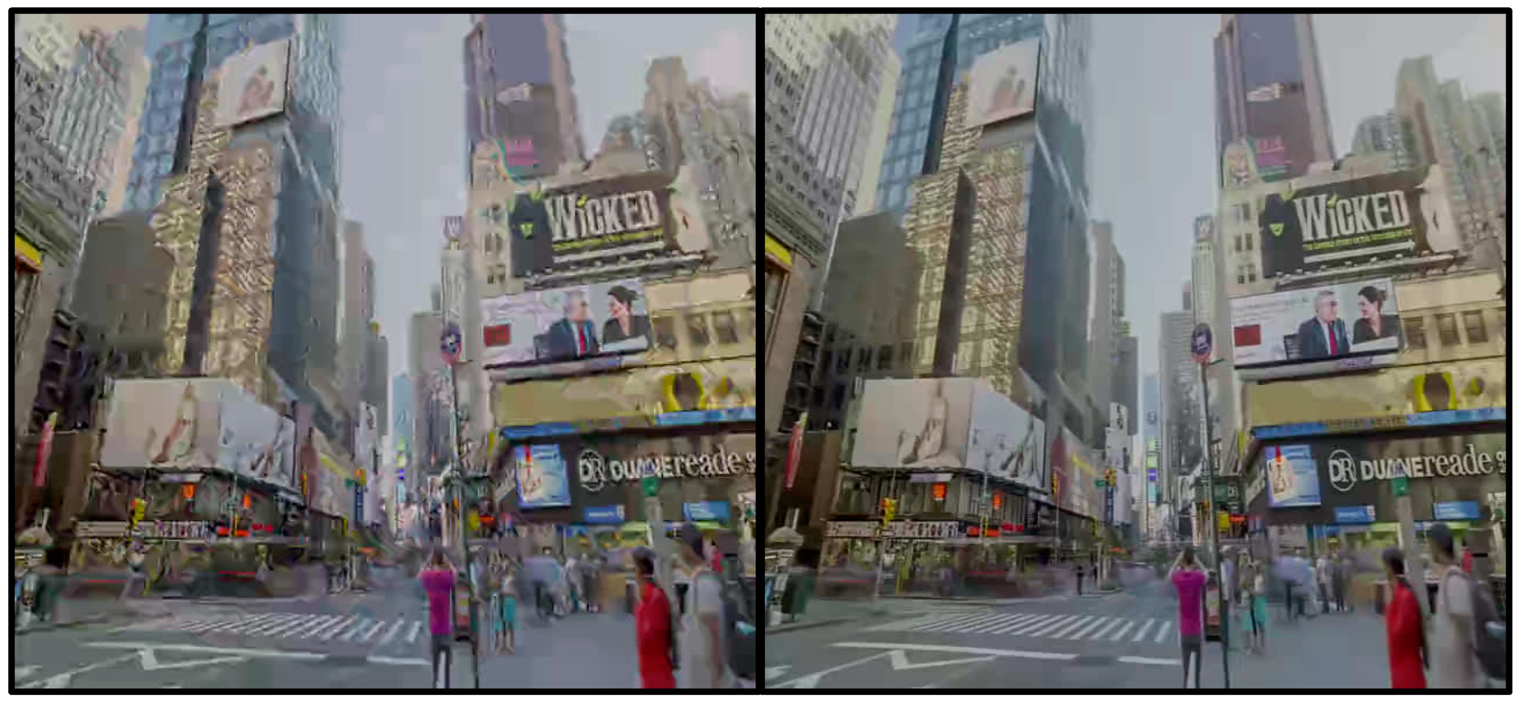
Figure 8.
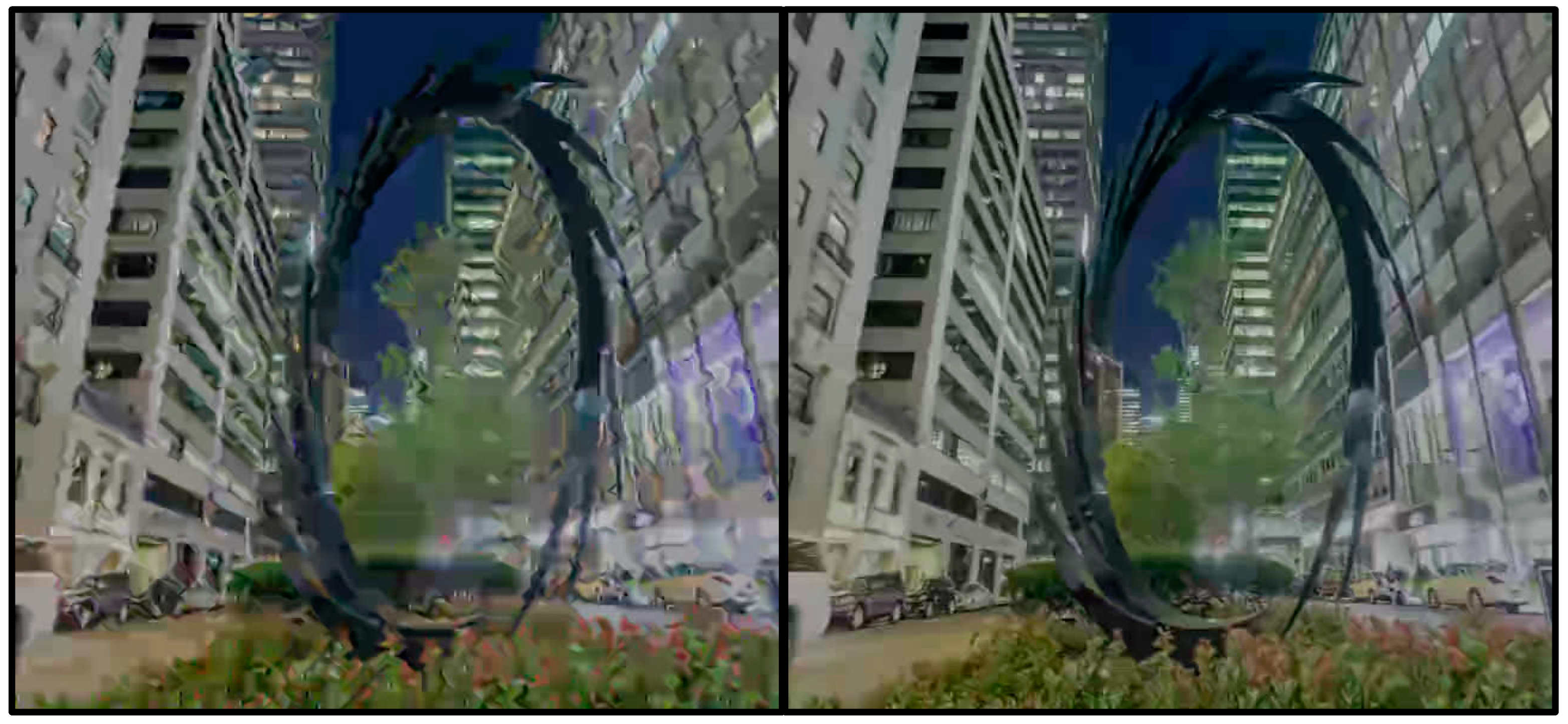
Preview of compression effects for frame 800 with QP=51 of the test video [61] (viewed from the left: the image compressed by pure AVC, and the image processed by ADNN and compressed by AVC).
Figure 8.
Preview of compression effects for frame 800 with QP=51 of the test video [61] (viewed from the left: the image compressed by pure AVC, and the image processed by ADNN and compressed by AVC).
4.2. HEVC Compression Enhancement Research Results
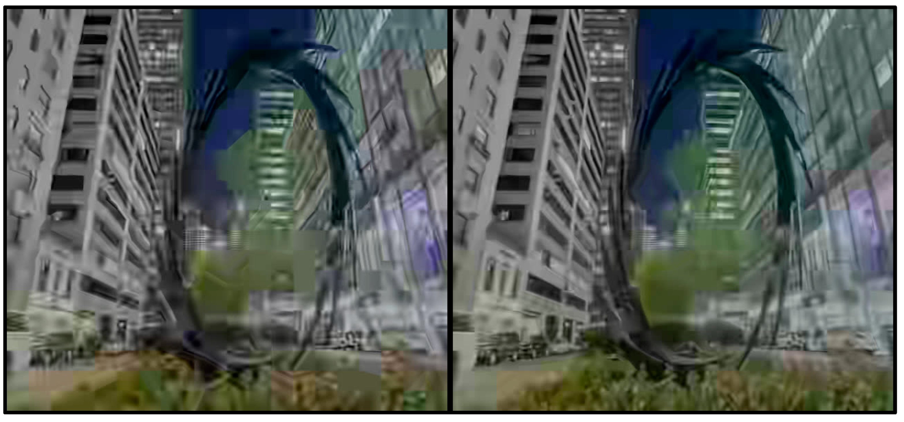
The results of ADNN processing in the context of improving the visual quality of video subjected to HEVC compression are presented in Table 9, Table 10 and Table 11, which show the averaged results of processing on sample test video frames [61] with the image resolution changed to 640 × 640. A graphical preview of ADNN processing in the context of improving video quality is shown in Figure 10, Figure 11, Figure 12, Figure 13, Figure 14 and Figure 15 and in Appendix A.
From the analysis of the results in Table 9, Table 10 and Table 11 and Figure 9, it is noticeable that there is no direct improvement and a slight deterioration of the PSNR value for ADNN compression in comparison to HEVC compression. This is due to the fact that ADNN makes more changes to the image than native HEVC compression. Similar to the previously discussed results for native AVC compression.
Based on the results of the study, it was found that the proposed method works effectively when there is no direct translation of the QP compression factor value fed to the ADNN input to the target QP compression value for HEVC compression. Starting from QP value 23 there is noticeable tendency to improve the quality of the video.
In order to properly present the use of ADNN capabilities, a conversion table (Table 12) was compiled on the basis of the conducted research, which presents suggested compression values for ADNN in relation to the target HEVC compression value. Similar to the previously discussed results for native AVC compression.
It should be emphasized that conversion values in Table 12 are used further in this manuscript to present further results in the context of the HEVC compression. Meaning that for a compression value, e.g. QP = 45, the value of the compression ratio at the ADNN input was given in accordance with conversion table (Table 12) as 38, and then processed image from ADNN was given for the HEVC video codec, for which the value of compression is QP = 38. Thus, keeping for the indicated value a larger number details with a similar output file size.
In order to utilize the conversion table (Table 12), it is needed to first determine the target compression ratio QP for HEVC, then read the corresponding QP value for ADNN from the table and use it in the calculations for the image preprocessing by ADNN.
The average gain of the proposed method in numerical form for specified QP value can be obtained by reading the values from Table 12. Average of ∇PSNR is 1.27 dB and the average value of file size reduction is 0.76 KB for QP value greater than 22. The graphical results of the ADNN processing are shown in Figure 10, Figure 11, Figure 12, Figure 13, Figure 14 and Figure 15.
Figure 10.
Preview of compression effects for frame 200 and 400 of the test video [61] with QP=41 (viewed from the top, the rows represent consecutive video frames, viewed from the left, the consecutive columns represent the original image, the image compressed by pure HEVC, and the image processed by ADNN and compressed by HEVC).
Figure 10.
Preview of compression effects for frame 200 and 400 of the test video [61] with QP=41 (viewed from the top, the rows represent consecutive video frames, viewed from the left, the consecutive columns represent the original image, the image compressed by pure HEVC, and the image processed by ADNN and compressed by HEVC).
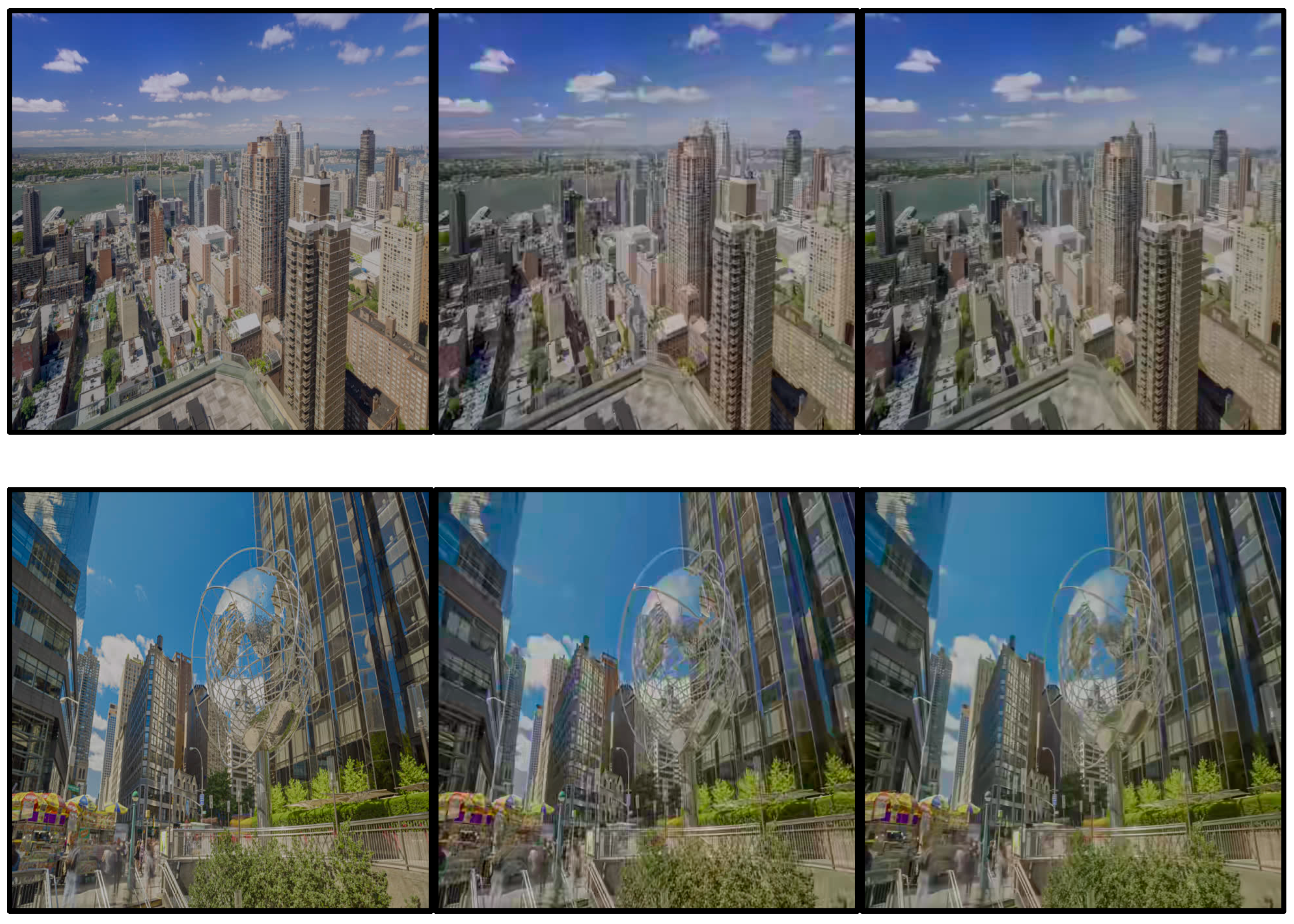
Figure 11.
Preview of compression effects for frame 600 and 800 of the test video [61] with QP=45 (viewed from the top, the rows represent consecutive video frames, viewed from the left, the consecutive columns represent the original image, the image compressed by pure HEVC, and the image processed by ADNN and compressed by HEVC).
Figure 11.
Preview of compression effects for frame 600 and 800 of the test video [61] with QP=45 (viewed from the top, the rows represent consecutive video frames, viewed from the left, the consecutive columns represent the original image, the image compressed by pure HEVC, and the image processed by ADNN and compressed by HEVC).
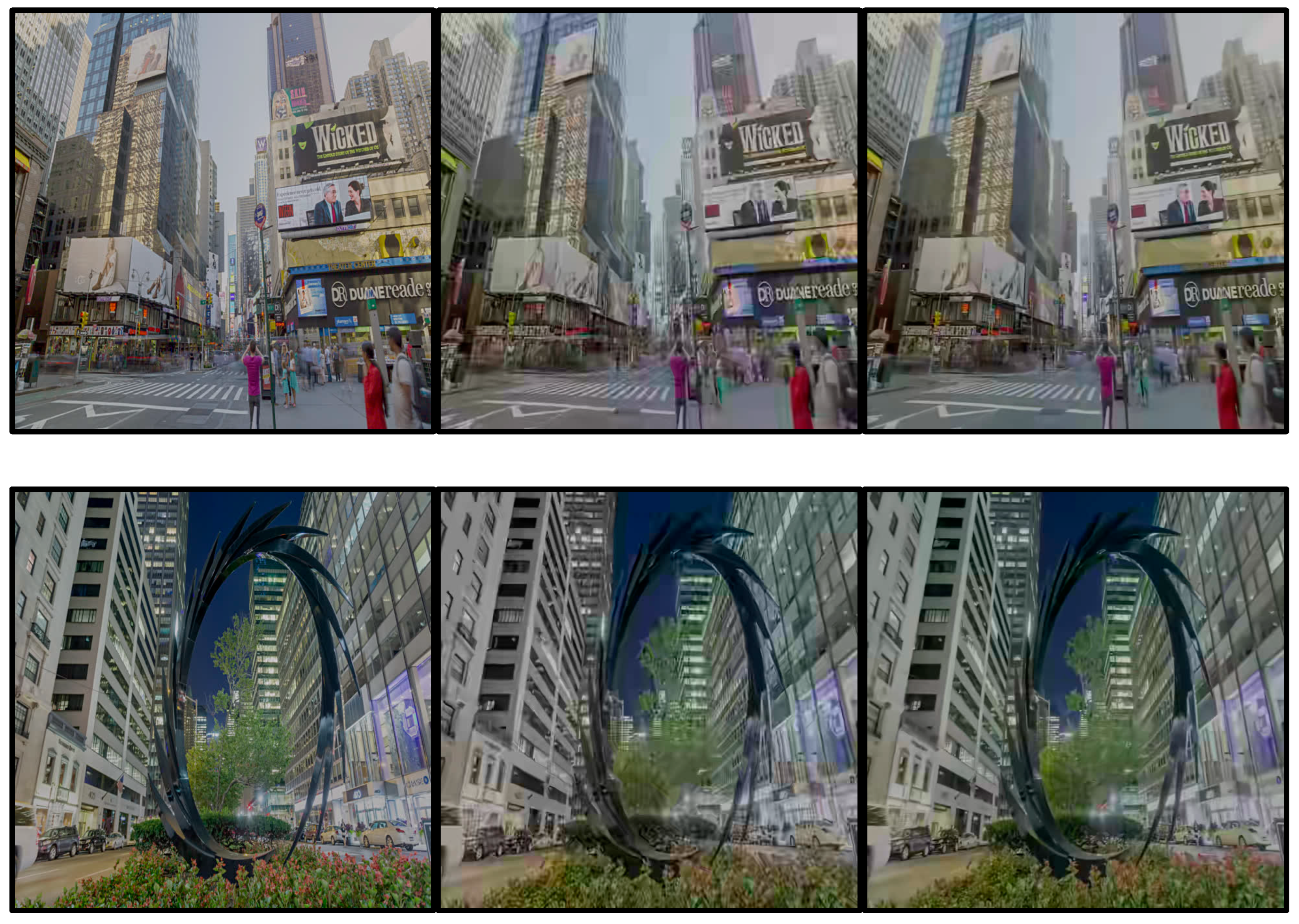
Figure 12.
Preview of compression effects for frame 600 and 800 of the test video [61] with QP=51 (viewed from the top, the rows represent consecutive video frames, viewed from the left, the consecutive columns represent the original image, the image compressed by pure HEVC, and the image processed by ADNN and compressed by HEVC).
Figure 12.
Preview of compression effects for frame 600 and 800 of the test video [61] with QP=51 (viewed from the top, the rows represent consecutive video frames, viewed from the left, the consecutive columns represent the original image, the image compressed by pure HEVC, and the image processed by ADNN and compressed by HEVC).
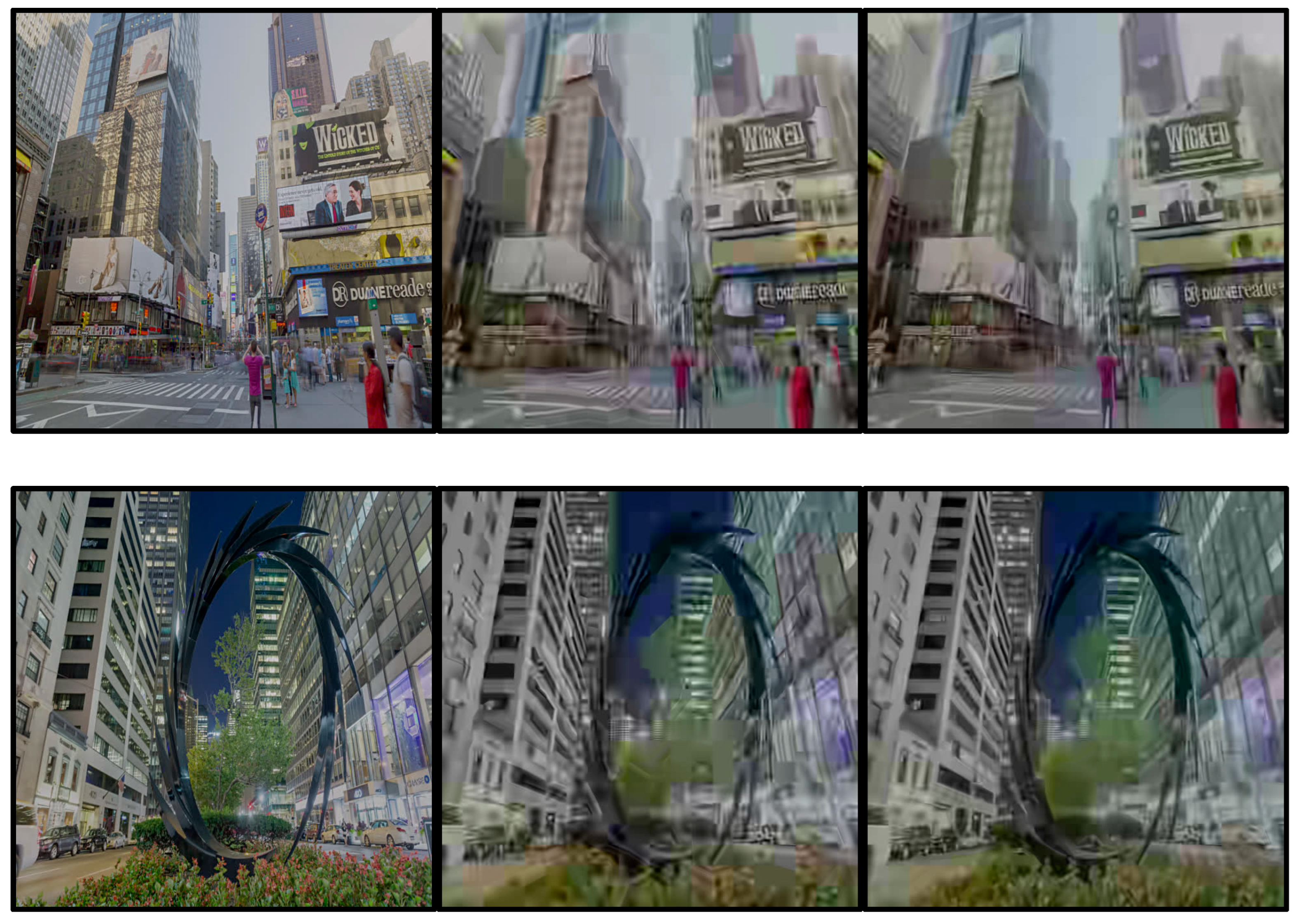
Figure 13.
Preview of compression effects for frame 200 with QP=43 of the test video [61] (viewed from the left: the image compressed by pure HEVC, and the image processed by ADNN and compressed by HEVC).
Figure 13.
Preview of compression effects for frame 200 with QP=43 of the test video [61] (viewed from the left: the image compressed by pure HEVC, and the image processed by ADNN and compressed by HEVC).
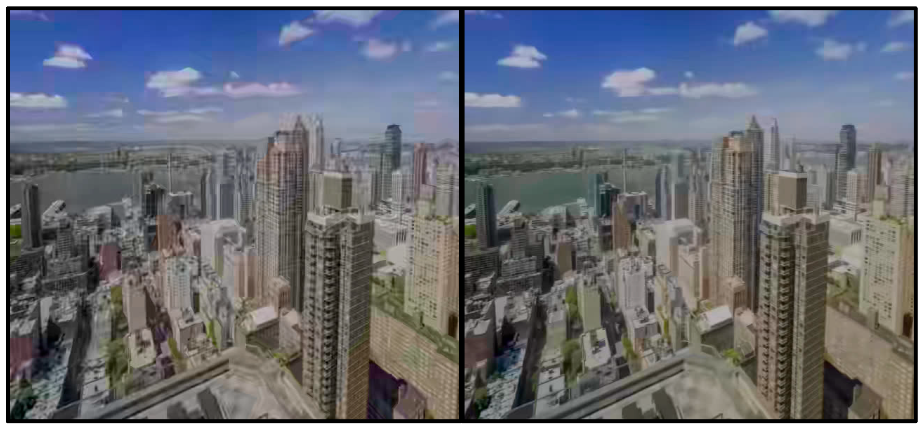
Figure 14.
Preview of compression effects for frame 600 with QP=47 of the test video [61] (viewed from the left: the image compressed by pure HEVC, and the image processed by ADNN and compressed by HEVC).
Figure 14.
Preview of compression effects for frame 600 with QP=47 of the test video [61] (viewed from the left: the image compressed by pure HEVC, and the image processed by ADNN and compressed by HEVC).
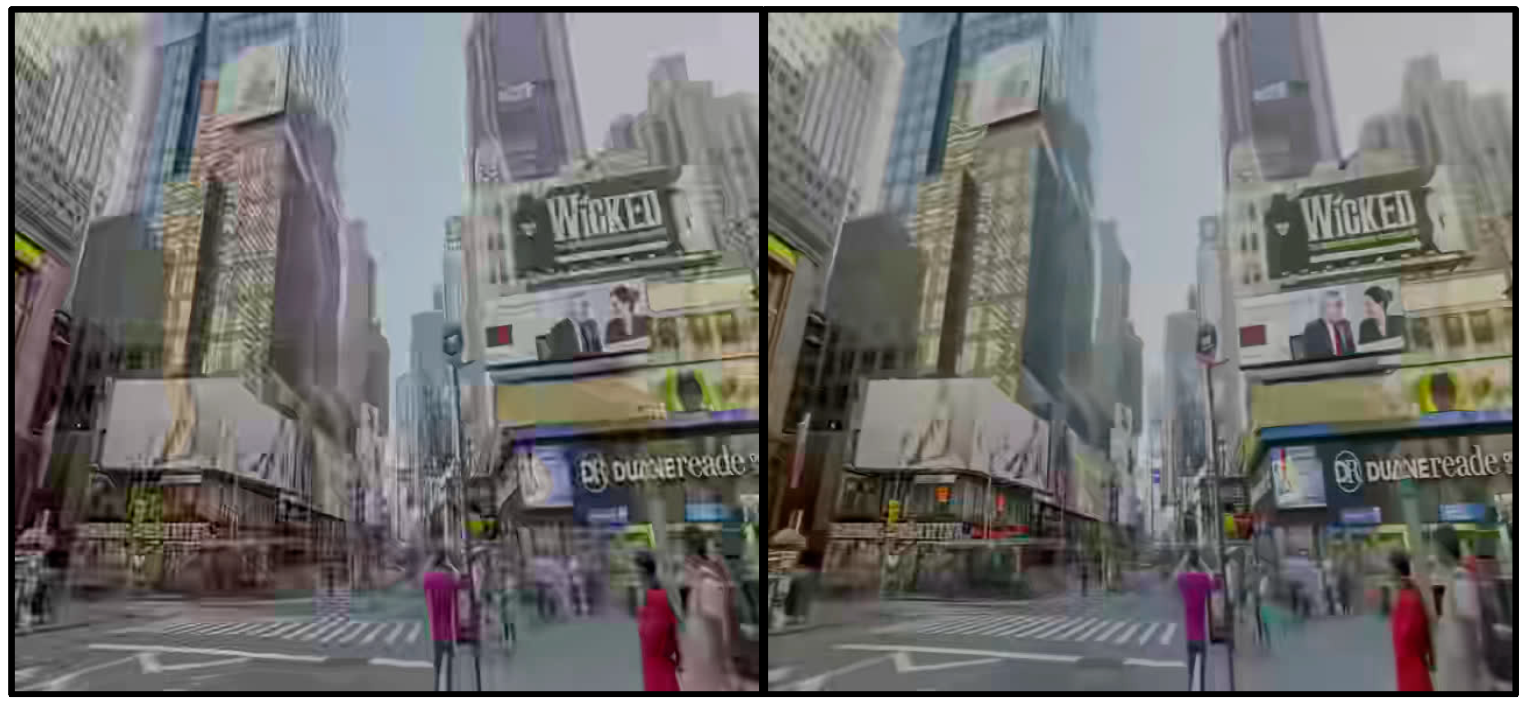
Figure 15.
Preview of compression effects for frame 800 with QP=51 of the test video [61] (viewed from the left: the image compressed by pure HEVC, and the image processed by ADNN and compressed by HEVC).
Figure 15.
Preview of compression effects for frame 800 with QP=51 of the test video [61] (viewed from the left: the image compressed by pure HEVC, and the image processed by ADNN and compressed by HEVC).
5. Conclusions
Improving the quality of video material after compression is a challenging issue. Improvement in image quality can be determined using various methods such as MSE, PSNR, or SSIM. However, it should be noted that mathematical calculations confirming or denying improvement in image quality may not take into account visible or invisible defects in the image that can be perceived by some viewers.
During the studies, it was found that there is an increase in the mathematical average PSNR value of approximately 2.03 dB for AVC and 1.27 dB for HEVC codec for each frame of video subjected to compression using AVC or HEVC starting from compression value (QP) value of 25 for AVC and 23 for HEVC. General tendency towards visual improvement in image quality with the use of the proposed method was confirmed from the compression values mentioned in the previous sentence up to its highest value of compression in its range of up to 51. The higher average gain values for AVC than HEVC are due to the fact that ADNN was trained using the compression characteristics of HEVC codec, which is a successor to AVC codec with stronger compression than AVC.
The proposed method results in a more accurate representation of color and details in the image. ADNN makes preliminary changes to the image preparing it for compression by taking into account the degradation characteristics caused by HEVC codec. In comparison to the popular trend of improving the quality of an already degraded image, the proposed method aims to improve the quality by trying to preserve it before compression algorithm is applied. The proposed method can be also used alongside with methods that corrects quality of images after decompression in order to obtain further quality improvement of decompressed video frames.
Further research on the proposed method should consider increasing the mathematical similarity of compressed image to original image for a wider range of compression offered by AVC and HEVC. To achieve this goal, further optimization of training process of neural network can be introduced. It is considered to use learning method based on use of Generative Adversarial Neural Networks (GAN) or Diffusion networks. GAN method will allow to pretrain ADNN in learning process of generator and discriminator to find in unsupervised manner dependencies (neural representations of codec characteristics) of AVC and HEVC processing, that can be later utilized to improve supervised mode of improvement image training.
Modification to the architecture of DNN model may allow for further optimizations. The use of models like IPCNN [47], DAIN [50] and SloMo [51] as part of ADNN structure may allow to capture or predict how frames will be modified after AVC and HEVC compression, and in this way more effectively adjust characteristics of video for coding process.
Next important thing to optimize will be objective function. Proper construction of objective function will allow to highlight for DNN (in training process) the key elements that impact perception of images quality. The approach with use only MSE and PSNR will not allow to further improvements of proposed method, because these quality indicators focus mainly on pixel-wise image differences and do not capture perceptually relevant differences. The objective function should be based on perceptual loss functions like SSIM, VIF, MOS which will be the nearest to human perception performance indicators.
Author Contributions
Conceptualization, M.K., D.P. and Z.P.; Funding acquisition, Z.P.; Methodology, M.K., D.P. and Z.P.; Project administration, Z.P.; Software, M.K. and D.P; Supervision, Z.P.; Visualization, M.K. and D.P; Writing—original draft, M.K., D.P and Z.P. All authors have read and agreed to the published version of the manuscript.
Funding
This research was funded by the Military University of Technology, Faculty of Electronics, grant number UGB/22-747 on Application of artificial intelligence methods to cognitive spectral analysis, satellite communications and watermarking and technology Deepfake.
Institutional Review Board Statement
Not applicable.
Informed Consent Statement
Not applicable.
Data Availability Statement
Conflicts of Interest
The authors declare no conflict of interest.
Appendix A
Figure A1.
Preview of compression effects for frame 600 with QP=47 of the test video [61] (viewed from the left: the images compressed by AVC and HEVC, viewed from top: the rows represent the images compressed by AVC and HEVC, and the image preprocessed by ADNN and then compressed accordingly by AVC or HEVC).
Figure A1.
Preview of compression effects for frame 600 with QP=47 of the test video [61] (viewed from the left: the images compressed by AVC and HEVC, viewed from top: the rows represent the images compressed by AVC and HEVC, and the image preprocessed by ADNN and then compressed accordingly by AVC or HEVC).
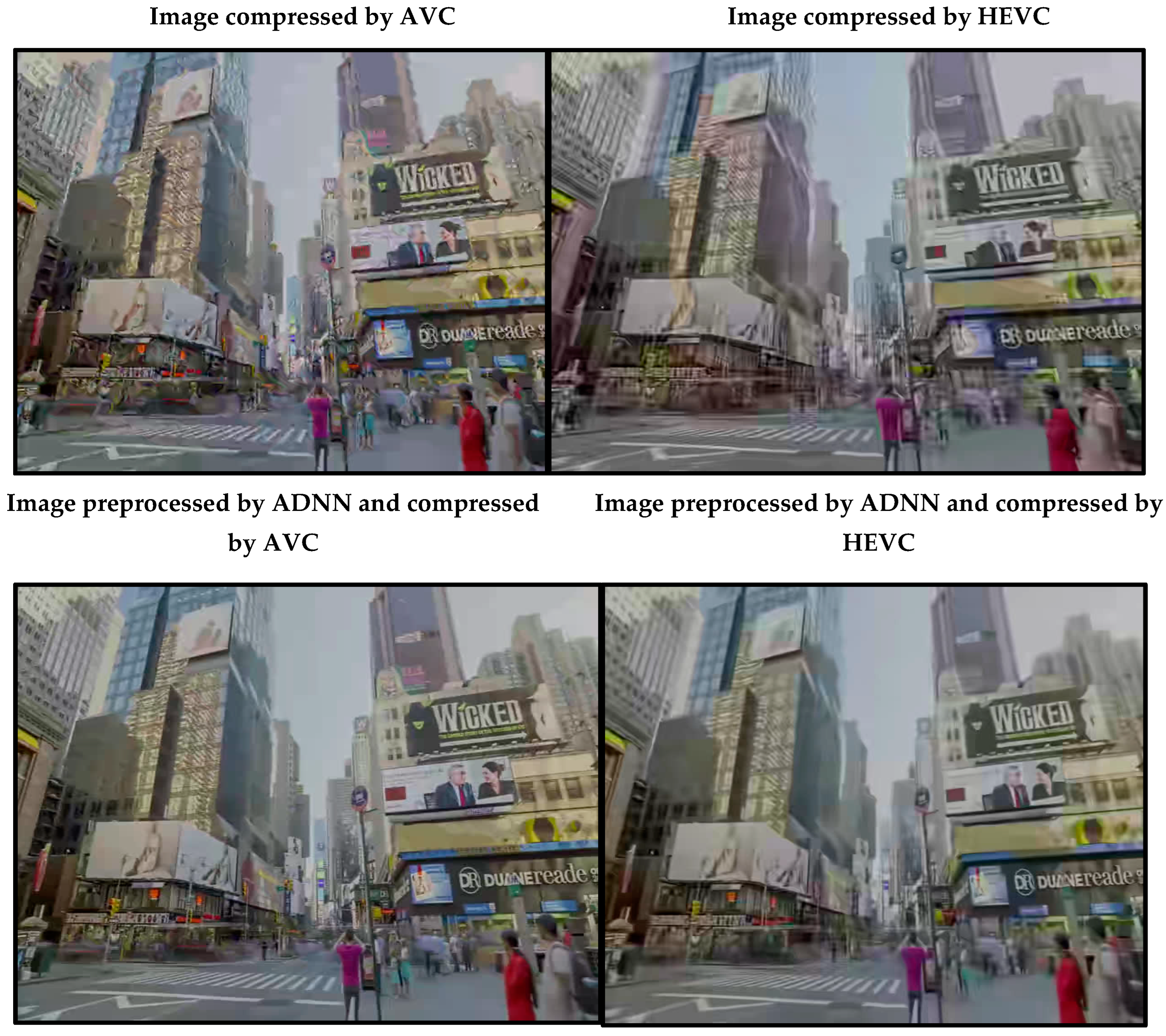
Figure A2.
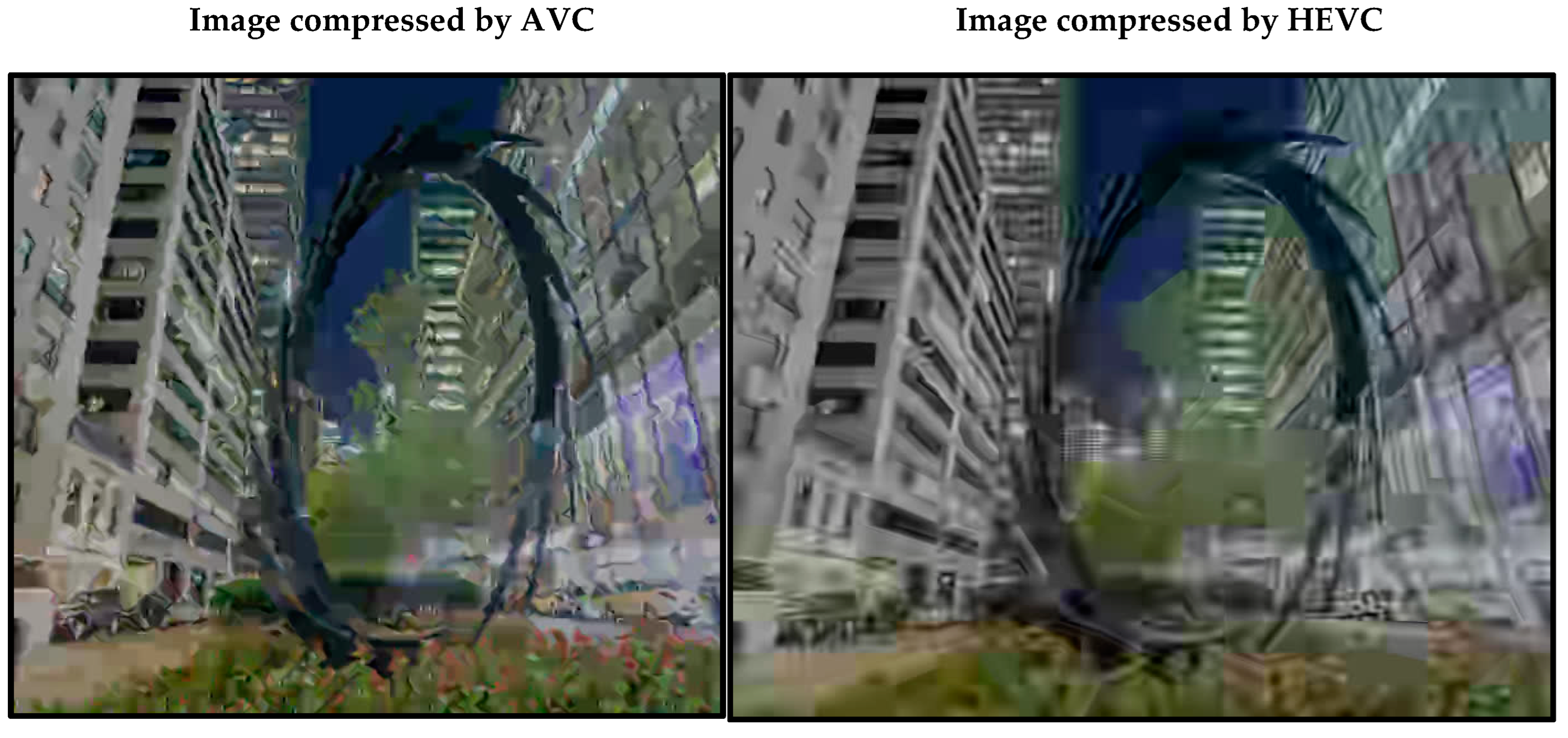
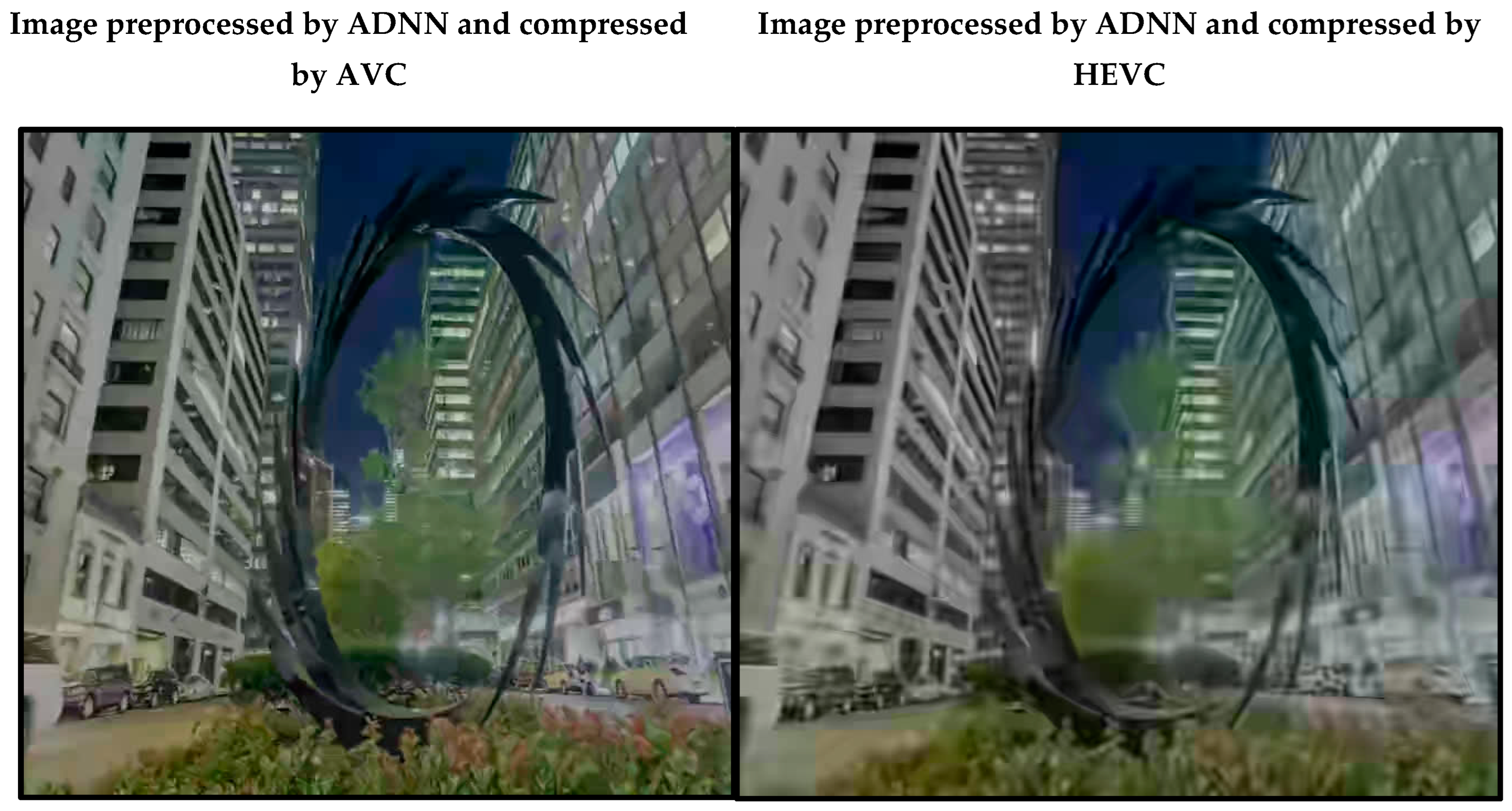
Preview of compression effects for frame 800 with QP=51 of the test video [61] (viewed from the left: the images compressed by AVC and HEVC, viewed from top: the rows represent the images compressed by AVC and HEVC, and the image preprocessed by ADNN and then compressed accordingly by AVC or HEVC).
Figure A2.
Preview of compression effects for frame 800 with QP=51 of the test video [61] (viewed from the left: the images compressed by AVC and HEVC, viewed from top: the rows represent the images compressed by AVC and HEVC, and the image preprocessed by ADNN and then compressed accordingly by AVC or HEVC).
References
- Schiopu, I.; Munteanu, A. Deep Learning Post-Filtering Using Multi-Head Attention and Multiresolution Feature Fusion for Image and Intra-Video Quality Enhancement. Sensors 2022, 22, 1353. [Google Scholar] [CrossRef]
- Jiang, X.; Song, T.; Zhu, D.; Katayama, T.; Wang, L. Quality-Oriented Perceptual HEVC Based on the Spatiotemporal Saliency Detection Model. Entropy 2019, 21, 165. [Google Scholar] [CrossRef] [PubMed]
- Wang, J.; Teng, G.; An, P. Video Super-Resolution Based on Generative Adversarial Network and Edge Enhancement. Electronics 2021, 10, 459. [Google Scholar] [CrossRef]
- Schiopu, I.; Munteanu, A. Attention Networks for the Quality Enhancement of Light Field Images. Sensors 2021, 21, 3246. [Google Scholar] [CrossRef] [PubMed]
- Si, L.; Wang, Z.; Xu, R.; Tan, C.; Liu, X.; Xu, J. Image Enhancement for Surveillance Video of Coal Mining Face Based on Single-Scale Retinex Algorithm Combined with Bilateral Filtering. Symmetry 2017, 9, 93. [Google Scholar] [CrossRef]
- Lopez-Vazquez, V.; Lopez-Guede, J.M.; Marini, S.; Fanelli, E.; Johnsen, E.; Aguzzi, J. Video Image Enhancement and Machine Learning Pipeline for Underwater Animal Detection and Classification at Cabled Observatories. Sensors 2020, 20, 726. [Google Scholar] [CrossRef]
- Caballero, J.; Ledig, C.; Aitken, A.; Acosta, A.; Totz, J.; Wang, Z.; Shi, W. Real-time video super-resolution with spatio-temporal networks and motion compensation. IEEE Conference on Computer Vision and Pattern Recognition, Honolulu, USA, 21–26 July 2017, pp. 2848–2857. [CrossRef]
- Huang, Y.; Wang, W.; Wang, L. Video superresolution via bidirectional recurrent convolutional networks. IEEE Transactions on Pattern Analysis and Machine Intelligence 2017, 40, 1015–1028. [Google Scholar] [CrossRef] [PubMed]
- Isobe, T.; Li, S.; Jia, X.; Yuan, S.; Slabaugh, G.; Xu, C.; Li, Y.; Wang, S.; Tian, Q. Video super-resolution with temporal group attention. IEEE Conference on Computer Vision and Pattern Recognition, Seattle, USA, 13–19 June 2020, pp. 7717–7727. [CrossRef]
- Kim, J.; Jung, Y.J. Multi-Stage Network for Event-Based Video Deblurring with Residual Hint Attention. Sensors 2023, 23, 2880. [Google Scholar] [CrossRef] [PubMed]
- Jiang, S.; Zhang, J.; Wang, W.; Wang, Y. Automatic Inspection of Bridge Bolts Using Unmanned Aerial Vision and Adaptive Scale Unification-Based Deep Learning. Remote Sens. 2023, 15, 328. [Google Scholar] [CrossRef]
- Li, J.; Gong, W.; Li, W. Combining Motion Compensation with Spatiotemporal Constraint for Video Deblurring. Sensors 2018, 18, 1774. [Google Scholar] [CrossRef]
- Mahdaoui, A.E.; Ouahabi, A.; Moulay, M.S. Image Denoising Using a Compressive Sensing Approach Based on Regularization Constraints. Sensors 2022, 22, 2199. [Google Scholar] [CrossRef]
- Lee, S.-Y.; Rhee, C.E. Motion Estimation-Assisted Denoising for an Efficient Combination with an HEVC Encoder. Sensors 2019, 19, 895. [Google Scholar] [CrossRef]
- Lee, M.S.; Park, S.W.; Kang, M.G. Denoising Algorithm for CFA Image Sensors Considering Inter-Channel Correlation. Sensors 2017, 17, 1236. [Google Scholar] [CrossRef]
- Chan, S.H.; Elgendy, O.A.; Wang, X. Images from Bits: Non-Iterative Image Reconstruction for Quanta Image Sensors. Sensors 2016, 16, 1961. [Google Scholar] [CrossRef]
- Min, X.; Zhai, G.; Gu, K.; Yang, X.; Guan, X. Objective Quality Evaluation of Dehazed Images. IEEE Transactions on Intelligent Transportation Systems 2019, 20, 2879–2892. [Google Scholar] [CrossRef]
- Min, X.; Zhai, G.; Gu, K.; Zhu, Y.; Zhou, J.; Guo, G.; Yang, X.; Guan, X.; Zhang, W. Quality Evaluation of Image Dehazing Methods Using Synthetic Hazy Images. IEEE Transactions on Multimedia 2019, 21, 2319–2333. [Google Scholar] [CrossRef]
- Li, Y.; Zhu, H.; He, L.; Wang, D.; Shi, J.; Wang, J. Video Super-Resolution with Regional Focus for Recurrent Network. Appl. Sci. 2023, 13, 526. [Google Scholar] [CrossRef]
- Shang, F.; Liu, H.; Ma, W.; Liu, Y.; Jiao, L.; Shang, F.; Wang, L.; Zhou, Z. Lightweight Super-Resolution with Self-Calibrated Convolution for Panoramic Videos. Sensors 2023, 23, 392. [Google Scholar] [CrossRef] [PubMed]
- Lee, Y.; Cho, S.; Jun, D. Video Super-Resolution Method Using Deformable Convolution-Based Alignment Network. Sensors 2022, 22, 8476. [Google Scholar] [CrossRef]
- Choi, J.; Oh, T.-H. Joint Video Super-Resolution and Frame Interpolation via Permutation Invariance. Sensors 2023, 23, 2529. [Google Scholar] [CrossRef] [PubMed]
- Tian, Y.; Zhang, Y.; Fu, Y.; Xu, C. Tdan: Temporally-deformable alignment network for video super-resolution. IEEE Conference on Computer Vision and Pattern Recognition, Seattle, USA, 13–19 June 2020, pp. 3357–3366. [CrossRef]
- Wang, X.; Chan, K.C.; Yu, K.; Dong, C.; Loy, C.C. EDVR: Video restoration with enhanced deformable convolutional networks. IEEE Conference on Computer Vision and Pattern Recognition Workshops, Long Beach, USA, 16–17 June 2019, pp. 1954–1963. [CrossRef]
- Zhou, S.; Zhang, J.; Pan, J.; Xie, H.; Zuo, W.; Ren, J. Spatio-temporal filter adaptive network for video deblurring. IEEE International Conference on Computer Vision, Seoul, Korea (South), pp. 2482–2491. 27 October–2 November 2019. [CrossRef]
- Dong, C.; Deng, Y.; Loy, C.C.; Tang, X. Compression artifacts reduction by a deep convolutional network. IEEE International Conference on Computer Vision, Santiago, Chile, 2015, 7–13 December 2015, pp. 576–584. [CrossRef]
- Xing, Q.; Xu, M.; Li, T.; Guan, Z. Early exit or not: Resource-efficient blind quality enhancement for compressed images. In European Conference on Computer Vision, Glasgow, Scotland, 23–28 August 2020, pp. 275–292. [CrossRef]
- Yang, R.; Xu, M.; Wang, Z. Decoder-side HEVC quality enhancement with scalable convolutional neural network. In 2017 IEEE International Conference on Multimedia and Expo (ICME), Hong Kong, China, 10–14 July 2017, pp. 817–822, 2017. [CrossRef]
- Kaczyński, M.; Piotrowski, Z. Lustrzany Kodek Video Bazujący na Głębokiej Sieci Neuronowej. Przegląd Telekomunikacyjny - Wiadomości Telekomunikacyjne 2024, 4, 395–398. [Google Scholar] [CrossRef]
- Chan, K. CK.; Wang, X.; Yu, K.; Dong, C.; Loy, CC. BasicVSR: The search for essential components in video super-resolution and beyond. IEEE Conference on Computer Vision and Pattern Recognition, Nashville, USA, 20–25 June 2021, pp. 4945–4954. [CrossRef]
- Chan, K.C.K.; Zhou, S.; Xu, X.; Loy, C.C. BasicVSR++: Improving video superresolution with enhanced propagation and alignment. Conference on Computer Vision and Pattern Recognition, New Orleans, USA, 18–24 June 2022, pp. 5962–5971. . [CrossRef]
- Lin, J.; Huang, Y.; Wang, L. FDAN: Flow-guided deformable alignment network for video super-resolution. 2021. [CrossRef]
- Son, H.; Lee, J.; Lee, J.; Cho, S.; Lee, S. Recurrent video deblurring with blur-invariant motion estimation and pixel volumes. ACM Transactions on Graphics 2021, 40, 1–18. [Google Scholar] [CrossRef]
- Zhong, Z.; Gao, Y.; Zheng, Y.; Zheng, B. Efficient spatio-temporal recurrent neural network for video deblurring. In European Conference on Computer Vision, Glasgow, Scotland, 23–28 August 2020, pp. 191–207. [CrossRef]
- Bistroń, M.; Piotrowski, Z. Efficient Video Watermarking Algorithm Based on Convolutional Neural Networks with Entropy-Based Information Mapper. Entropy 2023, 25, 284. [Google Scholar] [CrossRef]
- Walczyna, T.; Piotrowski, Z. Fast Fake: Easy-to-Train Face Swap Model. Appl. Sci. 2024, 14, 2149. [Google Scholar] [CrossRef]
- Jiang, L.; Wang, N.; Dang, Q.; Liu, R.; Lai, B. PP-MSVSR: multi-stage video super-resolution, 2021. [CrossRef]
- Mallik, B.; Sheikh-Akbari, A.; Bagheri Zadeh, P.; Al-Majeed, S. HEVC Based Frame Interleaved Coding Technique for Stereo and Multi-View Videos. Information 2022, 13, 554. [Google Scholar] [CrossRef]
- Zhou, M.; Wei, X.; Kwong, S.; Jia, W.; Fang, B. Rate Control Method Based on Deep Reinforcement Learning for Dynamic Video Sequences in HEVC. IEEE Transactions on Multimedia 2021, 23, 1106–1121. [Google Scholar] [CrossRef]
- Jacovi, A.; Hadash, G.; Kermany, E.; Carmeli, B.; Lavi, O.; Kour, G.; Berant, J. Neural Network Gradient-Based Learning of Black-Box Function Interfaces. 2019. [CrossRef]
- Sarafian, E.; Sinay, M.; Louzoun, Y.; Agmon, N.; Kraus, S. Explicit Gradient Learning for Black-Box Optimization. Proceedings of the 37th International Conference on Machine Learning in Proceedings of Machine Learning Research 2020, 119, 8480–8490. [Google Scholar]
- Grathwohl, W.; Choi, D.; Wu, Y.; Roeder, G.; Duvenaud, D. Backpropagation through the Void: Optimizing Control Variates for Black-Box Gradient Estimation. 2017. [CrossRef]
- Kaczyński, M.; Piotrowski, Z. High-Quality Video Watermarking Based on Deep Neural Networks and Adjustable Subsquares Properties Algorithm. Sensors 2022, 22, 5376. [Google Scholar] [CrossRef]
- Kaczyński, M.; Piotrowski, Z.; Pietrow, D. High-Quality Video Watermarking Based on Deep Neural Networks for Video with HEVC Compression. Sensors 2022, 22, 7552. [Google Scholar] [CrossRef]
- Lu, G.; Ouyang, W.; Xu, D.; Zhang, X.; Cai, C.; Gao, Z. DVC: An End-to-end Deep Video Compression Framework. 2018. [CrossRef]
- Chen, M.; Goodall, T.; Patney, A.; Bovik, A. C. Learning to Compress Videos without Computing Motion. In Signal Processing: Image Communication, 2022. [CrossRef]
- Cui, W.; Zhang, T.; Zhang, S.; Jiang, F.; Zuo, W.; Wan, Z.; Zhao, D. Convolutional Neural Networks Based Intra Prediction for HEVC. In 2017 Data Compression Conference (DCC), USA, 2017, pp. 436–436. [CrossRef]
- Laude, T.; Ostermann, J. Deep Learning Based Intra Prediction Mode Decision for HEVC. In 2016 Picture Coding Symposium (PCS), Germany, 2016, pp. 1–5. [CrossRef]
- Shimizu, J.; Cheng, Z.; Sun, H.; Takeuchi, M.; Katto, J. HEVC Video Coding with Deep Learning Based Frame Interpolation. In 2020 IEEE 9th Global Conference on Consumer Electronics (GCCE), Japan, 2020, pp. 433–434. [CrossRef]
- Bao, W.; Lai, W.; Ma, C.; Zhang, X.; Gao, Z.; Yang, M. Depth Aware Video Frame Interpolation. IEEE Conference on Computer Vision and Pattern Recognition, 15–20 June 2019. [CrossRef]
- Jiang, H.; Sun, D.; Jampani, V.; Yang, M.; Miller, E.; Kautz, J. Super SloMo: High Quality Estimation of Multiple Intermediate Frames for Video Interpolation. IEEE CVPR 2018. [CrossRef]
- Çetinkaya, E.; Amirpour, H.; Ghanbari, M.; Timmerer, C. CTU Depth Decision Algorithms for HEVC: A Survey. In Signal Processing: Image Communication, 2021, 99, 116442 Elsevier BV. [Google Scholar] [CrossRef]
- Zhai, G.; Min, X. Perceptual image quality assessment: a survey. Science China Information Sciences 2020, 63. [Google Scholar] [CrossRef]
- Wang, Z.; Bovik, A.C.; Sheikh, H.R. Image quality assessment: from error visibility to structural similarity. IEEE Trans Image Process 2004, 13, 600–612. [Google Scholar] [CrossRef] [PubMed]
- Min, X.; Gu, Ke.; Zhai, G.; Yang, X.; Zhang, W.; Le Callet, P.; Chen, C. W. Screen content quality assessment: Overview, benchmark, and beyond. ACM Computing Surveys 2021, 54, 1–36. [Google Scholar] [CrossRef]
- Min, X.; Zhai, G.; Zhou, J.; Farias, M. C. Q.; Bovik, A. C. Study of Subjective and Objective Quality Assessment of Audio-Visual Signals. IEEE Transactions on Image Processing 2020, 29, 6054–6068. [Google Scholar] [CrossRef]
- Sheikh, H. R.; Bovik, A. C. Image information and visual quality. IEEE Transactions on Image Processing 2006, 15, 430–444. [Google Scholar] [CrossRef]
- Bjontegaard, G. Improvements of the BD-PSNR Model. In ITUT SG 16, VCEG-AI11. 2008, pp. 1–2. Available online: https://www.itu.int/wftp3/av-arch/video-site/1707_Tor/VCEG-BD04-v1.doc (accessed on 11 November 2024).
- Senzaki, K. BD-PSNR/Rate Computation Tool for Five Data Points. In ITU-T SG 16 WP 3 and ISO/IEC JTC 1/SC 29/WG 11, JCTVC-B055. 2010, pp. 1–3. Available online: https://www.itu.int/wftp3/av-arch/JCTVC-site/2010_07_B_Geneva/JCTVC-B055.doc (accessed on 11 November 2024).
- Russakovsky, O.; Deng, J.; Su, H.; Krause, J.; Satheesh, S.; Ma, S.; Huang, Z.; Karpathy, A.; Khosla, A.; Bernstein, M.; Berg, A. C.; Fei-Fei, L. ImageNet Large Scale Visual Recognition Challenge. International Journal of Computer Vision 2015, 115, 211–252. [Google Scholar] [CrossRef]
- LG: New York HDR. Available online: https://4kmedia.org/lg-new-york-hdr-uhd-4k-demo/ (accessed on 11 November 2024).
- Khoreva, A.; Rohrbach, A.; Schiele, B. ; Video object segmentation with language referring expressions. In Asian Conference on Computer Vision. 2018. [Google Scholar] [CrossRef]
- Nah, S.; Kim, T.H.; Lee, K.M. Deep multi-scale convolutional neural network for dynamic scene deblurring. In IEEE Conference on Computer Vision and Pattern Recognition. 2017. [Google Scholar] [CrossRef]
- Nah, S.; Baik, S.; Hong, S.; Moon, G.; Son, S.; Timofte, R.; Lee, K.M. Ntire 2019 challenge on video deblurring and super-resolution: Dataset and study. In IEEE Conference on Computer Vision and Pattern Recognition Workshops. 2019. [Google Scholar]
- Xue, T.; Chen, B.; Wu, J.; Wei, D.; Freeman, W. Video enhancement with task-oriented flow. International Journal of Computer Vision. 2019. [Google Scholar] [CrossRef]
Figure 1.
Conceptual diagram of the method.

Figure 2.
Averaged enhancement results for a test video [61] processed with ADNN and compressed by AVC compared to the image compressed by pure AVC compression for PSNR and file size changes in QP.
Figure 2.
Averaged enhancement results for a test video [61] processed with ADNN and compressed by AVC compared to the image compressed by pure AVC compression for PSNR and file size changes in QP.
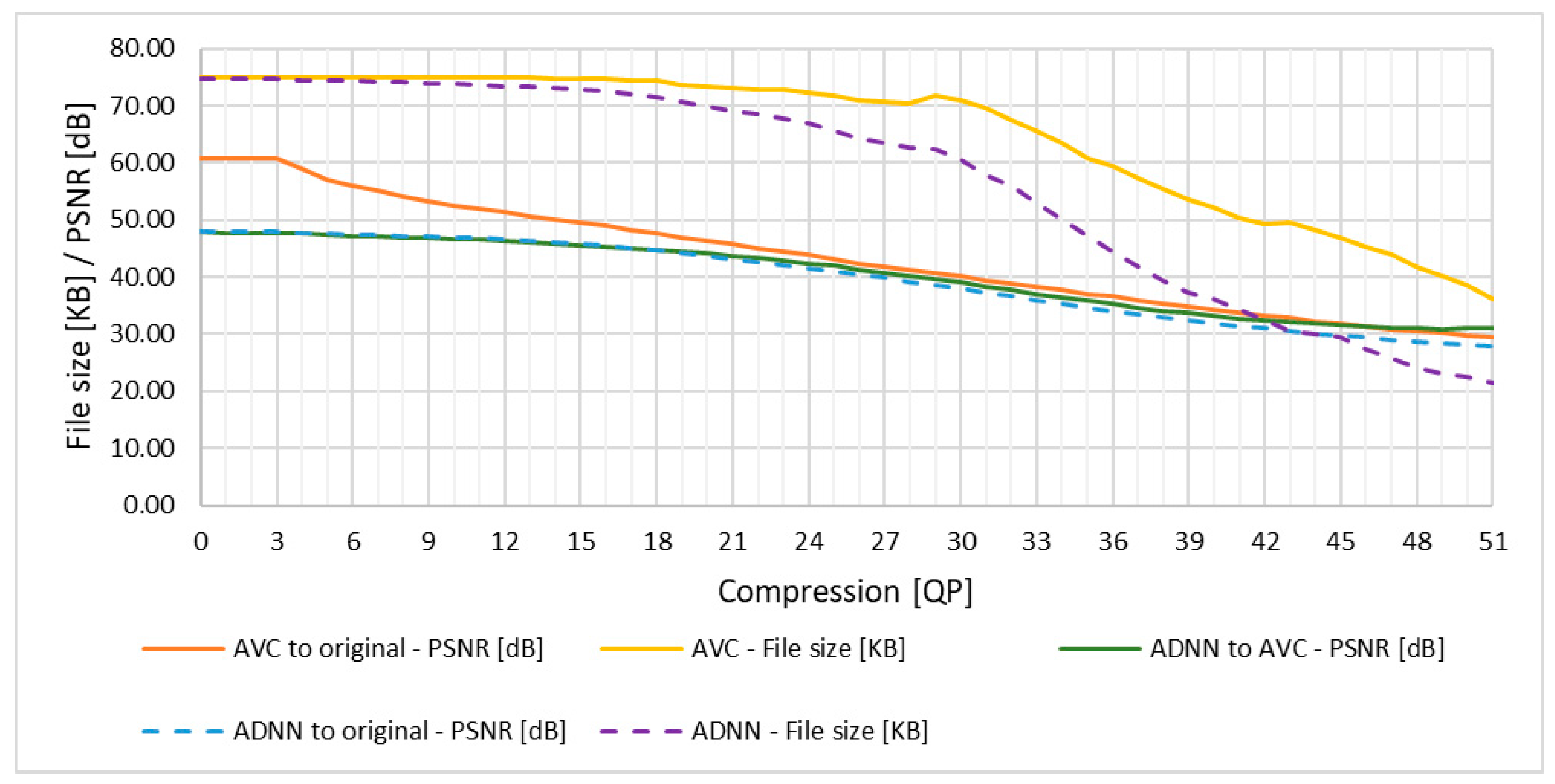
Figure 9.
Averaged enhancement results for a test video [61] processed with ADNN and compressed by HEVC compared to the image compressed by pure HEVC compression for PSNR and file size changes in QP.
Figure 9.
Averaged enhancement results for a test video [61] processed with ADNN and compressed by HEVC compared to the image compressed by pure HEVC compression for PSNR and file size changes in QP.
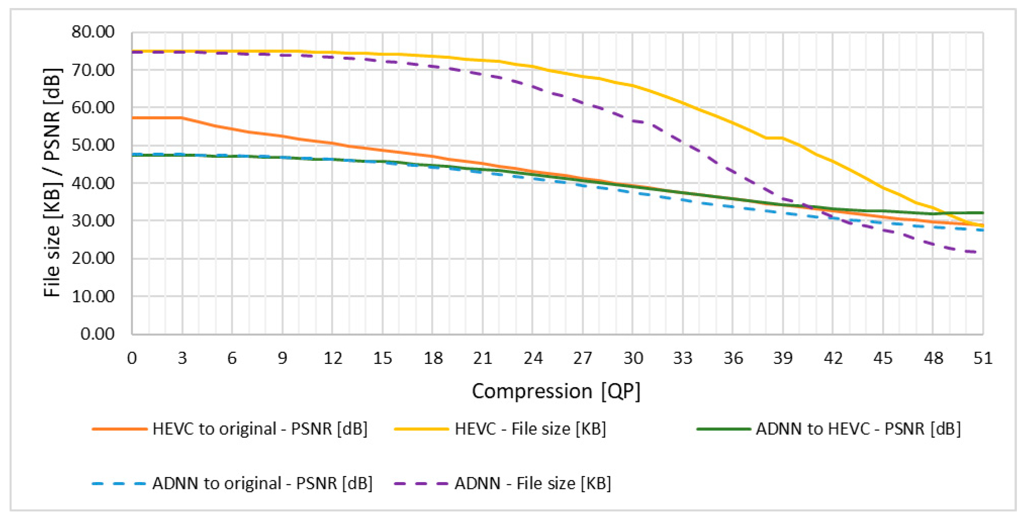

Table 1.
Convolution Basic Layer (CBL) – Logical layer model.
| Layer Number | Layer Type |
|---|---|
| 1 | DepthwiseConv2D(Input) |
| 2 | BatchNormalization(1) |
| 3 | Conv2D(2) |
| 4 | BatchNormalization(3) |
Table 2.
Transposed Convolution Basic Layer (TCBL) – Logical layer model.
| Layer Number | Layer Type |
|---|---|
| 1 | DepthwiseConv2D(Input) |
| 2 | BatchNormalization(1) |
| 3 | Conv2DTranspose(2) |
| 4 | BatchNormalization(3) |
Table 3.
A general model of convolutional neural network.
| Layer Number | Layer Type | Parameters |
|---|---|---|
| 1 | CBL(Input image) | activation function: GELU filter number: 156 Above set of properties is defined as: → Basic Parameters kernel size: 3 × 3 |
| 2 | CBL(1) | Basic Parameters kernel size: 4 × 4 |
| 3 | Multiply(2, Input QP value) | |
| 4 | Concatenate((2, 3), axis = 3) | |
| 5 | BatchNormalization(4) | - |
| 6 | CBL(5) | Basic Parameters kernel size: 4 × 4 |
| 7 | Concatenate((1, 6), axis = 3) | - |
| 8 | BatchNormalization(7) | - |
| 9 | TCBL(8) | Basic Parameters kernel size: 4 × 4 |
| 10 | TCBL(8) | Basic Parameters kernel size: 4 × 4 |
| 11 | Concatenate((9, 10), axis = 3) | - |
| 12 | BatchNormalization(11) | - |
| 13 | CBL(12) | Basic Parameters kernel size: 4 × 4 |
| 14 | CBL(12) | Basic Parameters kernel size: 4 × 4 |
| 15 | Concatenate((13, 14), axis = 3) | - |
| 16 | BatchNormalization(15) | - |
| 17 | CBL(16) | Basic Parameters kernel size: 4 × 4 |
| 18 | CBL(17) | Basic Parameters kernel size: 3 × 3 |
| 19 | Conv2D(18) | activation function: LeakyReLU kernel size: 1 |
Table 4.
Parameters of the neural network.
| Input Tensor Size |
Number of Parameters | Size on Disk | Processing Time for a Single Tensor [ms] |
|---|---|---|---|
| (128, 128, 3) | 5342421 | 62.80 MB | 52.33 |
Table 5.
Enhancement results for a test video [61] processed with ADNN and compressed by AVC compared to the image compressed by pure AVC compression for PSNR, SSIM and file size changes in QP.
Table 5.
Enhancement results for a test video [61] processed with ADNN and compressed by AVC compared to the image compressed by pure AVC compression for PSNR, SSIM and file size changes in QP.
| Frame # | Type | QP 0 | QP 16 | QP 23 | QP 28 | QP 31 | QP 41 | QP 51 |
|---|---|---|---|---|---|---|---|---|
| 200 69.30 KB1 |
Proposed method to AVC | PSNR2: 48.36 SSIM3: 0.999 |
PSNR: 45.93 SSIM: 0.993 |
PSNR: 43.71 SSIM: 0.988 |
PSNR: 41.07 SSIM: 0.981 |
PSNR: 39.03 SSIM: 0.971 |
PSNR: 33.83 SSIM: 0.922 |
PSNR: 32.79 SSIM: 0.909 |
| Proposed method to original image |
PSNR: 48.36 SSIM: 0.999 68.91 KB4 |
PSNR: 45.88 SSIM: 0.991 66.30 KB |
PSNR: 42.87 SSIM: 0.976 61.37 KB |
PSNR: 40.11 SSIM: 0.962 58.45 KB |
PSNR: 38.08 SSIM: 0.950 51.33 KB |
PSNR: 32.36 SSIM: 0.881 27.93 KB |
PSNR: 29.03 SSIM: 0.801 18.96 KB |
|
| AVC to original image |
PSNR: 60.76 SSIM: 0.999 69.30 KB |
PSNR: 49.30 SSIM: 0.994 68.77 KB |
PSNR: 45.07 SSIM: 0.983 66.27 KB |
PSNR: 42.09 SSIM: 0.973 65.78 KB |
PSNR: 40.27 SSIM: 0.965 62.60 KB |
PSNR: 34.56 SSIM: 0.925 44.32 KB |
PSNR: 30.60 SSIM: 0.852 27.94 KB |
|
| 400 77.34 KB |
Proposed method to AVC | PSNR: 47.97 SSIM: 0.999 |
PSNR: 45.17 SSIM: 0.993 |
PSNR: 42.47 SSIM: 0.983 |
PSNR: 39.94 SSIM: 0.972 |
PSNR: 38.09 SSIM: 0.962 |
PSNR: 32.30 SSIM: 0.887 |
PSNR: 31.30 SSIM: 0.843 |
| Proposed method to original image |
PSNR: 47.97 SSIM: 0.999 77.02 KB |
PSNR: 45.25 SSIM: 0.991 74.90 KB |
PSNR: 41.76 SSIM: 0.973 70.24 KB |
PSNR: 38.74 SSIM: 0.949 63.9 KB |
PSNR: 36.86 SSIM: 0.933 60.19 KB |
PSNR: 30.88 SSIM: 0.827 36.36 KB |
PSNR: 27.64 SSIM: 0.704 20.43 KB |
|
| AVC to original image |
PSNR: 60.87 SSIM: 0.999 77.34 KB |
PSNR: 48.66 SSIM: 0.995 77.13 KB |
PSNR: 44.00 SSIM: 0.983 75.45 KB |
PSNR: 40.72 SSIM: 0.967 72.19 KB |
PSNR: 39.02 SSIM: 0.958 72.22 KB |
PSNR: 33.31 SSIM: 0.903 52.13 KB |
PSNR: 29.13 SSIM: 0.802 37.74 KB |
|
| 600 74.51 KB |
Proposed method to AVC | PSNR: 48.14 SSIM: 0.999 |
PSNR: 45.29 SSIM: 0.992 |
PSNR: 42.77 SSIM: 0.985 |
PSNR: 40.22 SSIM: 0.975 |
PSNR: 38.39 SSIM: 0.966 |
PSNR: 32.60 SSIM: 0.909 |
PSNR: 30.43 SSIM: 0.859 |
| Proposed method to original image |
PSNR: 48.14 SSIM: 0.999 74.12 KB |
PSNR: 45.27 SSIM: 0.990 71.81 KB |
PSNR: 41.88 SSIM: 0.972 67.26 KB |
PSNR: 39.00 SSIM: 0.951 61.99 KB |
PSNR: 37.16 SSIM: 0.937 57.69 KB |
PSNR: 31.24 SSIM: 0.855 36.96 KB |
PSNR: 27.43 SSIM: 0.744 23.29 KB |
|
| AVC to original image |
PSNR: 61.10 SSIM: 0.999 74.51 KB |
PSNR: 48.58 SSIM: 0.993 74.16 KB |
PSNR: 44.03 SSIM: 0.981 72.28 KB |
PSNR: 40.96 SSIM: 0.967 69.57 KB |
PSNR: 39.27 SSIM: 0.958 68.94 KB |
PSNR: 33.59 SSIM: 0.912 50.47 KB |
PSNR: 29.14 SSIM: 0.830 39.4 KB |
|
| 800 79.19 KB |
Proposed method to AVC | PSNR: 47.67 SSIM: 0.999 |
PSNR: 45.12 SSIM: 0.994 |
PSNR: 42.43 SSIM: 0.985 |
PSNR: 39.93 SSIM: 0.972 |
PSNR: 38.13 SSIM: 0.961 |
PSNR: 32.39 SSIM: 0.904 |
PSNR: 30.12 SSIM: 0.850 |
| Proposed method to original image |
PSNR: 47.67 SSIM: 0.999 78.93 KB |
PSNR: 45.33 SSIM: 0.993 76.91 KB |
PSNR: 41.97 SSIM: 0.976 72.63 KB |
PSNR: 38.89 SSIM: 0.952 66.07 KB |
PSNR: 37.06 SSIM: 0.936 62.59 KB |
PSNR: 31.10 SSIM: 0.851 36.17 KB |
PSNR: 27.29 SSIM: 0.737 22.84 KB |
|
| AVC to original image |
PSNR: 60.86 SSIM: 0.999 79.19 KB |
PSNR: 49.07 SSIM: 0.996 78.9 KB |
PSNR: 44.39 SSIM: 0.985 77.18 KB |
PSNR: 41.03 SSIM: 0.971 74.24 KB |
PSNR: 39.27 SSIM: 0.962 74.27 KB |
PSNR: 33.36 SSIM: 0.910 54.56 KB |
PSNR: 28.87 SSIM: 0.823 39.38 KB |
1 File size of the original image in kilobytes saved in JPG format, 2 Peak signal-to-noise ratio, 3 Structural similarity index measure, 4 File size in kilobytes saved in JPG format.
Table 6.
Averaged enhancement results for frames with resolution of 128 × 128 of the test datasets processed with ADNN and compressed by AVC compared to the image compressed by AVC compression and original image for PSNR and SSIM changes in QP.
Table 6.
Averaged enhancement results for frames with resolution of 128 × 128 of the test datasets processed with ADNN and compressed by AVC compared to the image compressed by AVC compression and original image for PSNR and SSIM changes in QP.
| Frame # | Type | QP 1 | QP 16 | QP 23 | QP 28 | QP 31 | QP 41 | QP 51 |
|---|---|---|---|---|---|---|---|---|
| DAVIS [62] | ADNN to AVC | PSNR1: 47.77 SSIM2: 0.998 |
PSNR: 45.45 SSIM: 0.993 |
PSNR: 42.71 SSIM: 0.986 |
PSNR: 39.93 SSIM: 0.975 |
PSNR: 38.02 SSIM: 0.964 |
PSNR: 33.20 SSIM: 0.914 |
PSNR: 30.42 SSIM: 0.872 |
| ADNN to original image | PSNR: 47.90 SSIM: 0.998 |
PSNR: 45.48 SSIM: 0.991 |
PSNR: 42.14 SSIM: 0.977 |
PSNR: 38.99 SSIM: 0.958 |
PSNR: 37.00 SSIM: 0.943 |
PSNR: 31.60 SSIM: 0.868 |
PSNR: 27.75 SSIM: 0.778 |
|
| AVC to original image |
PSNR: 61.30 SSIM: 0.999 |
PSNR: 48.98 SSIM: 0.991 |
PSNR: 44.23 SSIM: 0.984 |
PSNR: 40.93 SSIM: 0.972 |
PSNR: 39.04 SSIM: 0.964 |
PSNR: 33.45 SSIM: 0.918 |
PSNR: 29.42 SSIM: 0.853 |
|
| GoPro [63] | ADNN to AVC | PSNR: 46.56 SSIM: 0.998 |
PSNR: 44.49 SSIM: 0.993 |
PSNR: 41.84 SSIM: 0.985 |
PSNR: 39.18 SSIM: 0.973 |
PSNR: 37.36 SSIM: 0.961 |
PSNR: 31.33 SSIM: 0.883 |
PSNR: 27.90 SSIM: 0.792 |
| ADNN to original image |
PSNR: 46.68 SSIM: 0.998 |
PSNR: 44.77 SSIM: 0.993 |
PSNR: 41.59 SSIM: 0.979 |
PSNR: 38.40 SSIM: 0.956 |
PSNR: 36.46 SSIM: 0.938 |
PSNR: 30.14 SSIM: 0.832 |
PSNR: 25.82 SSIM: 0.702 |
|
| AVC to original image |
PSNR: 61.06 SSIM: 0.999 |
PSNR: 48.88 SSIM: 0.995 |
PSNR: 43.98 SSIM: 0.986 |
PSNR: 40.44 SSIM: 0.973 |
PSNR: 38.56 SSIM: 0.965 |
PSNR: 32.42 SSIM: 0.916 |
PSNR: 27.74 SSIM: 0.845 |
|
| REDS [64] | ADNN to AVC | PSNR: 46.74 SSIM: 0.998 |
PSNR: 44.35 SSIM: 0.992 |
PSNR: 41.40 SSIM: 0.982 |
PSNR: 38.88 SSIM: 0.968 |
PSNR: 37.29 SSIM: 0.957 |
PSNR: 31.42 SSIM: 0.888 |
PSNR: 27.59 SSIM: 0.787 |
| ADNN to original image |
PSNR: 46.87 SSIM: 0.998 |
PSNR: 44.58 SSIM: 0.992 |
PSNR: 40.93 SSIM: 0.974 |
PSNR: 37.75 SSIM: 0.945 |
PSNR: 36.04 SSIM: 0.925 |
PSNR: 30.15 SSIM: 0.825 |
PSNR: 25.65 SSIM: 0.693 |
|
| AVC to original image |
PSNR: 61.06 SSIM: 0.999 |
PSNR: 48.39 SSIM: 0.994 |
PSNR: 43.21 SSIM: 0.983 |
PSNR: 39.71 SSIM: 0.966 |
PSNR: 37.98 SSIM: 0.956 |
PSNR: 32.23 SSIM: 0.904 |
PSNR: 27.55 SSIM: 0.838 |
|
| Vimeo-90K-T [65] | ADNN to AVC | PSNR: 48.57 SSIM: 0.998 |
PSNR: 46.58 SSIM: 0.994 |
PSNR: 44.52 SSIM: 0.989 |
PSNR: 42.25 SSIM: 0.981 |
PSNR: 40.65 SSIM: 0.974 |
PSNR: 34.87 SSIM: 0.930 |
PSNR: 30.33 SSIM: 0.871 |
| ADNN to original image |
PSNR: 48.70 SSIM: 0.998 |
PSNR: 46.81 SSIM: 0.994 |
PSNR: 43.98 SSIM: 0.985 |
PSNR: 41.18 SSIM: 0.970 |
PSNR: 39.52 SSIM: 0.959 |
PSNR: 33.77 SSIM: 0.897 |
PSNR: 28.72 SSIM: 0.811 |
|
| AVC to original image |
PSNR: 61.28 SSIM: 0.999 |
PSNR: 50.50 SSIM: 0.996 |
PSNR: 46.37 SSIM: 0.990 |
PSNR: 43.28 SSIM: 0.981 |
PSNR: 41.71 SSIM: 0.976 |
PSNR: 36.26 SSIM: 0.946 |
PSNR: 31.11 SSIM: 0.901 |
1 Peak signal-to-noise ratio, 2 Structural similarity index measure.
Table 7.
Averaged enhancement results for a test video [61] processed with ADNN and compressed by AVC compared to the image compressed by pure AVC compression for PSNR and file size changes in QP.
Table 7.
Averaged enhancement results for a test video [61] processed with ADNN and compressed by AVC compared to the image compressed by pure AVC compression for PSNR and file size changes in QP.
| QP | 0 | 1 | 2 | 3 | 4 | 5 | 6 | 7 | 8 | 9 | 10 | 11 | 12 |
| File size1 AVC | 75.09 | 75.05 | 75.04 | 75.04 | 75.04 | 74.98 | 74.96 | 74.96 | 74.90 | 74.95 | 74.97 | 74.86 | 74.87 |
| File size ADNN | 74.75 | 74.66 | 74.63 | 74.61 | 74.56 | 74.42 | 74.34 | 74.26 | 74.07 | 74.01 | 73.88 | 73.68 | 73.48 |
| PSNR2 AVC | 60.90 | 60.90 | 60.90 | 60.90 | 58.80 | 57.15 | 56.00 | 55.11 | 54.14 | 53.29 | 52.58 | 51.91 | 51.34 |
| PSNR ADNN | 48.04 | 47.87 | 47.87 | 47.86 | 47.75 | 47.63 | 47.51 | 47.42 | 47.23 | 47.12 | 46.93 | 46.74 | 46.56 |
| QP | 13 | 14 | 15 | 16 | 17 | 18 | 19 | 20 | 21 | 22 | 23 | 24 | 25 |
| File size AVC | 74.88 | 74.83 | 74.74 | 74.74 | 74.55 | 74.36 | 73.70 | 73.30 | 73.03 | 72.73 | 72.80 | 72.39 | 71.63 |
| File size ADNN | 73.29 | 73.08 | 72.75 | 72.48 | 71.97 | 71.48 | 70.62 | 69.83 | 69.11 | 68.54 | 67.88 | 66.84 | 65.50 |
| PSNR AVC | 50.70 | 50.11 | 49.51 | 48.90 | 48.28 | 47.71 | 46.91 | 46.30 | 45.69 | 45.08 | 44.37 | 43.81 | 43.10 |
| PSNR ADNN | 46.33 | 46.05 | 45.78 | 45.43 | 45.07 | 44.71 | 44.07 | 43.61 | 43.19 | 42.66 | 42.12 | 41.62 | 41.00 |
| QP | 26 | 27 | 28 | 29 | 30 | 31 | 32 | 33 | 34 | 35 | 36 | 37 | 38 |
| File size AVC | 71.00 | 70.56 | 70.45 | 71.74 | 70.88 | 69.51 | 67.37 | 65.56 | 63.49 | 60.88 | 59.48 | 57.29 | 55.42 |
| File size ADNN | 64.25 | 63.33 | 62.60 | 62.40 | 60.61 | 57.95 | 56.10 | 52.99 | 50.13 | 47.06 | 44.43 | 41.86 | 39.30 |
| PSNR AVC | 42.42 | 41.77 | 41.20 | 40.71 | 40.13 | 39.46 | 38.75 | 38.31 | 37.75 | 36.99 | 36.60 | 35.93 | 35.40 |
| PSNR ADNN | 40.38 | 39.77 | 39.19 | 38.61 | 38.03 | 37.29 | 36.58 | 35.98 | 35.38 | 34.65 | 34.12 | 33.49 | 32.94 |
| QP | 39 | 40 | 41 | 42 | 43 | 44 | 45 | 46 | 47 | 48 | 49 | 50 | 51 |
| File size AVC | 53.53 | 52.09 | 50.37 | 49.27 | 49.50 | 48.18 | 46.77 | 45.19 | 43.83 | 41.74 | 40.08 | 38.54 | 36.12 |
| File size ADNN | 37.30 | 36.28 | 34.36 | 32.50 | 30.47 | 29.92 | 29.37 | 27.45 | 25.76 | 24.18 | 23.02 | 22.60 | 21.38 |
| PSNR AVC | 34.83 | 34.39 | 33.71 | 33.32 | 32.81 | 32.24 | 31.83 | 31.43 | 30.90 | 30.56 | 30.16 | 29.78 | 29.44 |
| PSNR ADNN | 32.39 | 31.92 | 31.40 | 30.96 | 30.51 | 30.08 | 29.69 | 29.33 | 28.93 | 28.63 | 28.34 | 28.11 | 27.85 |
1 File size in kilobytes saved in JPG format, 2 Peak signal-to-noise ratio.
Table 8.
Conversion table of the target AVC compression ratio with corresponding ∇PSNR and ∇file size results for a test video [61].
Table 8.
Conversion table of the target AVC compression ratio with corresponding ∇PSNR and ∇file size results for a test video [61].
| QP AVC | 0 | 1 | 2 | 3 | 4 | 5 | 6 | 7 | 8 | 9 | 10 | 11 | 12 |
| QP ADNN | 0 | 0 | 0 | 0 | 0 | 0 | 0 | 0 | 0 | 0 | 0 | 0 | 0 |
| ∇PSNR1 | -12.86 | -12.86 | -12.86 | -12.86 | -10.77 | -9.11 | -7.97 | -7.07 | -6.11 | -5.25 | -4.55 | -3.88 | -3.31 |
| ∇File size2 | 0.34 | -0.30 | -0.29 | -0.29 | -0.29 | -0.23 | -0.21 | -0.21 | -0.15 | -0.20 | -0.22 | -0.11 | -0.13 |
| QP AVC | 13 | 14 | 15 | 16 | 17 | 18 | 19 | 20 | 21 | 22 | 23 | 24 | 25 |
| QP ADNN | 0 | 0 | 0 | 0 | 0 | 0 | 0 | 0 | 0 | 0 | 0 | 0 | 18 |
| ∇PSNR | -2.66 | -2.08 | -1.47 | -0.87 | -0.24 | 0.32 | 1.13 | 1.73 | 2.35 | 2.96 | 3.66 | 4.22 | 1.60 |
| ∇File size | -0.13 | -0.08 | 0.01 | 0.01 | 0.20 | 0.38 | 1.05 | 1.45 | 1.72 | 2.01 | 1.95 | 2.36 | -0.15 |
| QP AVC | 26 | 27 | 28 | 29 | 30 | 31 | 32 | 33 | 34 | 35 | 36 | 37 | 38 |
| QP ADNN | 19 | 20 | 20 | 20 | 20 | 21 | 24 | 25 | 27 | 30 | 31 | 32 | 33 |
| ∇PSNR | 1.65 | 1.85 | 2.41 | 2.90 | 3.48 | 3.74 | 2.87 | 2.69 | 2.02 | 1.04 | 0.69 | 0.65 | 0.58 |
| ∇File size | -0.39 | -0.73 | -0.61 | -1.91 | -1.05 | -0.40 | -0.53 | -0.06 | -0.16 | -0.28 | -1.53 | -1.20 | -2.43 |
| QP AVC | 39 | 40 | 41 | 42 | 43 | 44 | 45 | 46 | 47 | 48 | 49 | 50 | 51 |
| QP ADNN | 33 | 34 | 34 | 35 | 35 | 35 | 36 | 36 | 37 | 38 | 38 | 39 | 41 |
| ∇PSNR | 1.15 | 0.99 | 1.68 | 1.33 | 1.84 | 2.41 | 2.29 | 2.69 | 2.59 | 2.38 | 2.78 | 2.61 | 1.96 |
| ∇File size | -0.54 | -1.96 | -0.24 | -2.22 | -2.44 | -1.13 | -2.34 | -0.76 | -1.97 | -2.44 | -0.78 | -1.24 | -1.76 |
1 Peak signal-to-noise ratio, 2 File size in kilobytes saved in JPG format.
Table 9.
Enhancement results for a test video [61] processed with ADNN and compressed by HEVC compared to the image compressed by pure HEVC compression for PSNR, SSIM and file size changes in QP.
Table 9.
Enhancement results for a test video [61] processed with ADNN and compressed by HEVC compared to the image compressed by pure HEVC compression for PSNR, SSIM and file size changes in QP.
| Frame # | Type | QP 0 | QP 16 | QP 23 | QP 28 | QP 31 | QP 41 | QP 51 |
|---|---|---|---|---|---|---|---|---|
| 200 69.30 KB1 |
Proposed method to HEVC | PSNR2: 47.76 SSIM3: 0.999 |
PSNR: 46.05 SSIM: 0.994 |
PSNR: 43.64 SSIM: 0.986 |
PSNR: 40.99 SSIM: 0.977 |
PSNR: 39.33 SSIM: 0.971 |
PSNR: 34.83 SSIM: 0.941 |
PSNR: 33.13 SSIM: 0.920 |
| Proposed method to original image |
PSNR: 47.94 SSIM: 0.999 68.91 KB4 |
PSNR: 45.63 SSIM: 0.989 65.95 KB |
PSNR: 42.71 SSIM: 0.974 60.80 KB |
PSNR: 39.72 SSIM: 0.957 54.52 KB |
PSNR: 37.72 SSIM: 0.944 48.44 KB |
PSNR: 32.19 SSIM: 0.877 26.94 KB |
PSNR: 28.91 SSIM: 0.799 19.81 KB |
|
| HEVC to original image |
PSNR: 57.29 SSIM: 0.999 69.31 KB |
PSNR: 48.82 SSIM: 0.993 68.17 KB |
PSNR: 44.80 SSIM: 0.981 65.13 KB |
PSNR: 41.65 SSIM: 0.968 61.99 KB |
PSNR: 39.75 SSIM: 0.957 58.50 KB |
PSNR: 34.21 SSIM: 0.912 40.94 KB |
PSNR: 30.19 SSIM: 0.839 24.23 KB |
|
| 400 77.34 KB |
Proposed method to HEVC | PSNR: 47.34 SSIM: 0.999 |
PSNR: 45.14 SSIM: 0.993 |
PSNR: 42.41 SSIM: 0.982 |
PSNR: 39.83 SSIM: 0.968 |
PSNR: 38.04 SSIM: 0.958 |
PSNR: 33.08 SSIM: 0.907 |
PSNR: 32.47 SSIM: 0.894 |
| Proposed method to original image |
PSNR: 47.58 SSIM: 0.999 76.95 KB |
PSNR: 44.79 SSIM: 0.989 74.37 KB |
PSNR: 41.40 SSIM: 0.970 69.11 KB |
PSNR: 38.37 SSIM: 0.945 61.97 KB |
PSNR: 36.39 SSIM: 0.924 62.95 KB |
PSNR: 30.57 SSIM: 0.811 34.48 KB |
PSNR: 27.49 SSIM: 0.696 20.82 KB |
|
| HEVC to original image |
PSNR: 57.21 SSIM: 0.999 77.38 KB |
PSNR: 47.87 SSIM: 0.993 76.49 KB |
PSNR: 43.40 SSIM: 0.979 74.07 KB |
PSNR: 40.19 SSIM: 0.962 69.83 KB |
PSNR: 38.26 SSIM: 0.945 66.85 KB |
PSNR: 32.53 SSIM: 0.865 53.41 KB |
PSNR: 28.46 SSIM: 0.746 27.69 KB |
|
| 600 74.51 KB |
Proposed method to HEVC | PSNR: 47.49 SSIM: 0.999 |
PSNR: 45.34 SSIM: 0.992 |
PSNR: 42.72 SSIM: 0.983 |
PSNR: 40.22 SSIM: 0.972 |
PSNR: 38.51 SSIM: 0.964 |
PSNR: 33.36 SSIM: 0.925 |
PSNR: 31.67 SSIM: 0.900 |
| Proposed method to original image |
PSNR: 47.73 SSIM: 0.999 74.11 KB |
PSNR: 44.85 SSIM: 0.987 71.17 KB |
PSNR: 41.56 SSIM: 0.969 66.21 KB |
PSNR: 38.64 SSIM: 0.947 59.67 KB |
PSNR: 36.74 SSIM: 0.930 54.20 KB |
PSNR: 30.91 SSIM: 0.843 35.55 KB |
PSNR: 27.28 SSIM: 0.738 22.73 KB |
|
| HEVC to original image |
PSNR: 57.31 SSIM: 0.999 74.55 KB |
PSNR: 47.83 SSIM: 0.991 73.37 KB |
PSNR: 43.51 SSIM: 0.978 70.86 KB |
PSNR: 40.43 SSIM: 0.961 66.96 KB |
PSNR: 38.60 SSIM: 0.947 64.00 KB |
PSNR: 32.92 SSIM: 0.883 47.27 KB |
PSNR: 28.47 SSIM: 0.786 30.62 KB |
|
| 800 79.19 KB |
Proposed method to HEVC | PSNR: 47.12 SSIM: 0.999 |
PSNR: 45.15 SSIM: 0.994 |
PSNR: 42.45 SSIM: 0.982 |
PSNR: 39.88 SSIM: 0.968 |
PSNR: 38.23 SSIM: 0.959 |
PSNR: 33.38 SSIM: 0.934 |
PSNR: 31.62 SSIM: 0.902 |
| Proposed method to original image |
PSNR: 47.31 SSIM: 0.999 78.94 KB |
PSNR: 45.01 SSIM: 0.991 76.38 KB |
PSNR: 41.63 SSIM: 0.973 71.22 KB |
PSNR: 38.54 SSIM: 0.947 64.06 KB |
PSNR: 36.57 SSIM: 0.927 58.04 KB |
PSNR: 30.85 SSIM: 0.843 35.07 KB |
PSNR: 27.19 SSIM: 0.735 23.01KB |
|
| HEVC to original image |
PSNR: 57.13 SSIM: 0.999 79.13 KB |
PSNR: 48.39 SSIM: 0.994 78.35 KB |
PSNR: 43.78 SSIM: 0.981 75.86 KB |
PSNR: 40.44 SSIM: 0.964 71.88 KB |
PSNR: 38.45 SSIM: 0.948 68.48 KB |
PSNR: 32.71 SSIM: 0.879 49.23 KB |
PSNR: 28.31 SSIM: 0.784 32.28 KB |
1 File size of the original image in kilobytes saved in JPG format, 2 Peak signal-to-noise ratio, 3 Structural similarity index measure, 4 File size in kilobytes saved in JPG format.
Table 10.
Averaged enhancement results for frames with resolution of 128 × 128 of the test datasets processed with ADNN and compressed by HEVC compared to the image compressed by HEVC compression and original image for PSNR and SSIM changes in QP.
Table 10.
Averaged enhancement results for frames with resolution of 128 × 128 of the test datasets processed with ADNN and compressed by HEVC compared to the image compressed by HEVC compression and original image for PSNR and SSIM changes in QP.
| Frame # | Type | QP 1 | QP 16 | QP 23 | QP 28 | QP 31 | QP 41 | QP 51 |
|---|---|---|---|---|---|---|---|---|
| DAVIS [76] | ADNN to HEVC | PSNR1: 47.47 SSIM2: 0.997 |
PSNR: 45.40 SSIM: 0.992 |
PSNR: 42.54 SSIM: 0.984 |
PSNR: 39.89 SSIM: 0.973 |
PSNR: 38.26 SSIM: 0.964 |
PSNR: 33.98 SSIM: 0.930 |
PSNR: 32.00 SSIM: 0.915 |
| ADNN to original image | PSNR: 47.67 SSIM: 0.997 |
PSNR: 45.10 SSIM: 0.989 |
PSNR: 41.78 SSIM: 0.975 |
PSNR: 38.59 SSIM: 0.954 |
PSNR: 36.60 SSIM: 0.936 |
PSNR: 31.23 SSIM: 0.855 |
PSNR: 27.62 SSIM: 0.768 |
|
| HEVC to original image |
PSNR: 57.64 SSIM: 0.999 |
PSNR: 48.30 SSIM: 0.992 |
PSNR: 43.75 SSIM: 0.981 |
PSNR: 40.41 SSIM: 0.967 |
PSNR: 38.42 SSIM: 0.954 |
PSNR: 32.78 SSIM: 0.889 |
PSNR: 28.72 SSIM: 0.803 |
|
| GoPro [77] | ADNN to HEVC | PSNR: 46.36 SSIM: 0.997 |
PSNR: 44.50 SSIM: 0.993 |
PSNR: 41.75 SSIM: 0.984 |
PSNR: 38.97 SSIM: 0.967 |
PSNR: 37.18 SSIM: 0.953 |
PSNR: 32.17 SSIM: 0.909 |
PSNR: 29.95 SSIM: 0.895 |
| ADNN to original image |
PSNR: 46.53 SSIM: 0.998 |
PSNR: 44.50 SSIM: 0.992 |
PSNR: 41.25 SSIM: 0.977 |
PSNR: 37.99 SSIM: 0.950 |
PSNR: 35.86 SSIM: 0.926 |
PSNR: 29.59 SSIM: 0.803 |
PSNR: 25.61 SSIM: 0.683 |
|
| HEVC to original image |
PSNR: 57.56 SSIM: 0.999 |
PSNR: 48.37 SSIM: 0.994 |
PSNR: 43.49 SSIM: 0.984 |
PSNR: 39.90 SSIM: 0.967 |
PSNR: 37.71 SSIM: 0.951 |
PSNR: 31.25 SSIM: 0.847 |
PSNR: 26.83 SSIM: 0.737 |
|
| REDS [78] | ADNN to HEVC | PSNR: 46.48 SSIM: 0.997 |
PSNR: 44.22 SSIM: 0.992 |
PSNR: 41.34 SSIM: 0.981 |
PSNR: 38.77 SSIM: 0.964 |
PSNR: 37.18 SSIM: 0.951 |
PSNR: 32.04 SSIM: 0.906 |
PSNR: 29.76 SSIM: 0.892 |
| ADNN to original image |
PSNR: 46.69 SSIM: 0.998 |
PSNR: 44.10 SSIM: 0.990 |
PSNR: 40.49 SSIM: 0.970 |
PSNR: 37.41 SSIM: 0.94 |
PSNR: 35.53 SSIM: 0.914 |
PSNR: 29.51 SSIM: 0.793 |
PSNR: 25.41 SSIM: 0.674 |
|
| HEVC to original image |
PSNR: 57.38 SSIM: 0.999 |
PSNR: 47.50 SSIM: 0.992 |
PSNR: 42.57 SSIM: 0.980 |
PSNR: 39.71 SSIM: 0.960 |
PSNR: 37.17 SSIM: 0.942 |
PSNR: 31.07 SSIM: 0.838 |
PSNR: 26.57 SSIM: 0.762 |
|
| Vimeo-90K-T [79] | ADNN to HEVC | PSNR: 48.40 SSIM: 0.998 |
PSNR: 46.66 SSIM: 0.994 |
PSNR: 44.33 SSIM: 0.988 |
PSNR: 41.93 SSIM: 0.978 |
PSNR: 40.29 SSIM: 0.969 |
PSNR: 35.11 SSIM: 0.939 |
PSNR: 31.49 SSIM: 0.921 |
| ADNN to original image |
PSNR: 48.54 SSIM: 0.998 |
PSNR: 46.61 SSIM: 0.993 |
PSNR: 43.64 SSIM: 0.983 |
PSNR: 40.81 SSIM: 0.966 |
PSNR: 38.97 SSIM: 0.951 |
PSNR: 33.04 SSIM: 0.874 |
PSNR: 28.35 SSIM: 0.793 |
|
| HEVC to original image |
PSNR: 58.70 SSIM: 0.999 |
PSNR: 50.18 SSIM: 0.995 |
PSNR: 45.91 SSIM: 0.988 |
PSNR: 42.75 SSIM: 0.977 |
PSNR: 40.85 SSIM: 0.967 |
PSNR: 34.76 SSIM: 0.903 |
PSNR: 29.83 SSIM: 0.828 |
1 Peak signal-to-noise ratio, 2 Structural similarity index measure.
Table 11.
Averaged enhancement results for a test video [61] processed with ADNN and compressed by HEVC compared to the image compressed by pure HEVC compression for PSNR and file size changes in QP.
Table 11.
Averaged enhancement results for a test video [61] processed with ADNN and compressed by HEVC compared to the image compressed by pure HEVC compression for PSNR and file size changes in QP.
| QP | 0 | 1 | 2 | 3 | 4 | 5 | 6 | 7 | 8 | 9 | 10 | 11 | 12 |
| File size1 HEVC | 75.09 | 75.09 | 75.09 | 75.09 | 75.08 | 75.08 | 75.07 | 75.07 | 75.04 | 74.97 | 74.95 | 74.81 | 74.72 |
| File size ADNN | 74.73 | 74.70 | 74.66 | 74.66 | 74.60 | 74.54 | 74.45 | 74.26 | 74.19 | 73.95 | 73.82 | 73.58 | 73.33 |
| PSNR2 HEVC | 57.24 | 57.24 | 57.24 | 57.24 | 56.16 | 55.16 | 54.34 | 53.62 | 52.95 | 52.37 | 51.74 | 51.14 | 50.58 |
| PSNR ADNN | 47.64 | 47.63 | 47.62 | 47.62 | 47.52 | 47.41 | 47.31 | 47.20 | 47.00 | 46.85 | 46.66 | 46.46 | 46.25 |
| QP | 13 | 14 | 15 | 16 | 17 | 18 | 19 | 20 | 21 | 22 | 23 | 24 | 25 |
| File size HEVC | 74.49 | 74.42 | 74.21 | 74.10 | 73.92 | 73.69 | 73.40 | 72.95 | 72.57 | 72.19 | 71.48 | 70.91 | 69.92 |
| File size ADNN | 73.02 | 72.72 | 72.29 | 71.97 | 71.50 | 70.99 | 70.32 | 69.59 | 68.78 | 67.91 | 66.84 | 65.59 | 64.12 |
| PSNR HEVC | 49.91 | 49.36 | 48.81 | 48.23 | 47.62 | 47.05 | 46.43 | 45.79 | 45.18 | 44.53 | 43.87 | 43.25 | 42.61 |
| PSNR ADNN | 45.98 | 45.68 | 45.41 | 45.07 | 44.69 | 44.31 | 43.88 | 43.39 | 42.89 | 42.37 | 41.83 | 41.27 | 40.69 |
| QP | 26 | 27 | 28 | 29 | 30 | 31 | 32 | 33 | 34 | 35 | 36 | 37 | 38 |
| File size HEVC | 68.98 | 68.30 | 67.67 | 66.68 | 65.89 | 64.46 | 62.91 | 61.34 | 59.42 | 57.82 | 56.02 | 54.09 | 52.07 |
| File size ADNN | 62.83 | 61.43 | 60.06 | 58.42 | 56.52 | 55.91 | 53.36 | 50.98 | 48.37 | 45.64 | 43.21 | 40.62 | 38.24 |
| PSNR HEVC | 41.95 | 41.33 | 40.68 | 40.01 | 39.39 | 38.77 | 38.14 | 37.57 | 36.95 | 36.34 | 35.79 | 35.22 | 34.67 |
| PSNR ADNN | 40.08 | 39.47 | 38.82 | 38.17 | 37.51 | 36.86 | 36.19 | 35.57 | 34.94 | 34.34 | 33.72 | 33.15 | 32.61 |
| QP | 39 | 40 | 41 | 42 | 43 | 44 | 45 | 46 | 47 | 48 | 49 | 50 | 51 |
| File size HEVC | 51.93 | 50.00 | 47.71 | 45.74 | 43.67 | 41.34 | 38.89 | 36.88 | 34.68 | 33.60 | 31.57 | 29.72 | 28.71 |
| File size ADNN | 35.88 | 34.88 | 33.01 | 31.03 | 29.37 | 28.71 | 27.61 | 26.74 | 25.20 | 23.78 | 22.67 | 22.06 | 21.59 |
| PSNR HEVC | 34.16 | 33.64 | 33.09 | 32.58 | 32.09 | 31.59 | 31.14 | 30.65 | 30.19 | 29.80 | 29.44 | 29.14 | 28.86 |
| PSNR ADNN | 32.09 | 31.61 | 31.13 | 30.69 | 30.26 | 29.88 | 29.50 | 29.09 | 28.72 | 28.39 | 28.12 | 27.92 | 27.72 |
1 File size in kilobytes saved in JPG format, 2 Peak signal-to-noise ratio.
Table 12.
Conversion table of the target HEVC compression ratio with corresponding ∇PSNR and ∇file size results for a test video [61].
Table 12.
Conversion table of the target HEVC compression ratio with corresponding ∇PSNR and ∇file size results for a test video [61].
| QP AVC | 0 | 1 | 2 | 3 | 4 | 5 | 6 | 7 | 8 | 9 | 10 | 11 | 12 |
| QP ADNN | 0 | 0 | 0 | 0 | 0 | 0 | 0 | 0 | 0 | 0 | 0 | 0 | 0 |
| ∇PSNR1 | -9.60 | -9.60 | -9.60 | -9.60 | -8.52 | -7.52 | -6.70 | -5.98 | -5.31 | -4.73 | -4.10 | -3.50 | -2.94 |
| ∇File size2 | -0.36 | -0.36 | -0.36 | -0.36 | -0.35 | -0.35 | -0.34 | -0.34 | -0.31 | -0.24 | -0.22 | -0.08 | 0.01 |
| QP AVC | 13 | 14 | 15 | 16 | 17 | 18 | 19 | 20 | 21 | 22 | 23 | 24 | 25 |
| QP ADNN | 0 | 0 | 0 | 0 | 0 | 0 | 0 | 0 | 0 | 0 | 18 | 19 | 20 |
| ∇PSNR | -2.27 | -1.72 | -1.17 | -0.59 | 0.02 | 0.59 | 1.22 | 1.85 | 2.46 | 3.11 | 0.44 | 0.63 | 0.78 |
| ∇File size | 0.24 | 0.31 | 0.52 | 0.63 | 0.81 | 1.04 | 1.33 | 1.78 | 2.16 | 2.54 | -0.49 | -0.59 | -0.33 |
| QP AVC | 26 | 27 | 28 | 29 | 30 | 31 | 32 | 33 | 34 | 35 | 36 | 37 | 38 |
| QP ADNN | 21 | 22 | 22 | 23 | 24 | 25 | 26 | 28 | 29 | 30 | 31 | 32 | 33 |
| ∇PSNR | 0.95 | 1.04 | 1.69 | 1.82 | 1.88 | 1.93 | 1.94 | 1.25 | 1.22 | 1.17 | 1.07 | 0.97 | 0.90 |
| ∇File size | -0.20 | -0.39 | -0.83 | -1.09 | -0.30 | -0.34 | -0.09 | -1.28 | -1.00 | -1.30 | -0.11 | -0.73 | -1.09 |
| QP AVC | 39 | 40 | 41 | 42 | 43 | 44 | 45 | 46 | 47 | 48 | 49 | 50 | 51 |
| QP ADNN | 33 | 34 | 35 | 35 | 36 | 37 | 38 | 39 | 41 | 41 | 42 | 43 | 45 |
| ∇PSNR | 1.41 | 1.31 | 1.24 | 1.76 | 1.64 | 1.56 | 1.48 | 1.44 | 0.95 | 1.33 | 1.25 | 1.12 | 0.64 |
| ∇File size | -0.95 | -1.63 | -2.08 | -0.10 | -0.46 | -0.71 | -0.65 | -1.01 | -1.67 | -0.59 | -0.54 | -0.35 | -1.09 |
1 Peak signal-to-noise ratio, 2 File size in kilobytes saved in JPG format.
Disclaimer/Publisher’s Note: The statements, opinions and data contained in all publications are solely those of the individual author(s) and contributor(s) and not of MDPI and/or the editor(s). MDPI and/or the editor(s) disclaim responsibility for any injury to people or property resulting from any ideas, methods, instructions or products referred to in the content. |
© 2024 by the authors. Licensee MDPI, Basel, Switzerland. This article is an open access article distributed under the terms and conditions of the Creative Commons Attribution (CC BY) license (http://creativecommons.org/licenses/by/4.0/).
Copyright: This open access article is published under a Creative Commons CC BY 4.0 license, which permit the free download, distribution, and reuse, provided that the author and preprint are cited in any reuse.


