
Submitted:
22 January 2025
Posted:
23 January 2025
You are already at the latest version
Abstract
In recent years, deep learning-based malware detection systems have been widely used in the field of cybersecurity, especially to detect malicious files in critical infrastructures. This paper proposes a lightweight malware detection method that can identify recent malware while being suitable for execution on embedded devices. This method combines the features of convolutional neural networks (CNN) with the tokenization advantages of transformer models. The proposed model architecture combines a diverse set of neural network layers designed to capture intricate patterns indicative of malicious behavior in files. Extensive experiments conducted using the latest CIC- Malmem-2022 dataset demonstrate that our method surpasses existing machine learning-based models in the literature for both malware detection and specific attack type identification. The model achieved a test accuracy of 99.97, demonstrating its high effectiveness in distinguishing between benign and malicious files. By combining dense neural networks, specialized capsule layers, and attention mechanisms, our architecture offers a robust solution for malware detection.
Keywords:
obfuscated memory malware (OMM)
; lightweight malware detection
; convolutional neural networks (CNN)
; bidirectional long short-term memory (BiLSTM)
; embedded IoT devices
Introduction
Recent progress in hardware and software technologies has made digital devices extremely powerful. Individuals and companies are highly dependent on servers and computers for daily information exchange and processing over the Internet. In 2017, there were an estimated 3.5 billion Internet users and this number is rapidly increasing. Despite the optimistic outlook for the digital technology sector, the consequences are significant. Due to economic incentives, digital devices are constantly threatened by malicious software (malware). The main defense against these malicious threats is a malware detection system provided by antivirus (AV) devices, which determines whether a file is malicious or benign. Traditional malware detection systems utilize basic machine learning algorithms such as decision trees, support vector machines, and naive Bayes classifiers. The effectiveness of these algorithms greatly depends on the quality of the features extracted. However, the process of feature selection and extraction is labor intensive, prone to errors, and requires extensive expertise., The new wave of machine learning algorithms, deep learning, has gained traction for its capability to automatically extract complex high-level features, leading to high accuracy. Most current deep learning-based malware detection systems primarily employ recurring neural networks (RNNs) with API calls and machine instructions as input. Despite the high accuracy of RNNs, they are susceptible to adversarial attacks, where attackers imitate RNNs RNN used in malware detection systems. By inserting redundant API calls, a malicious file can easily evade RNN detection, highlighting concerns about the robustness and effectiveness of RNNs for malware detection. This project aimed to evaluate the resilience of a hybrid model architecture against redundant API injections. The model integrates various layers, including dense layers, batch normalization, dropout, and custom layers like a Capsule Layer and Transformer Encoder. The process starts by converting the input file into an image and employing a CNN to learn its attributes and textures. As CNNs typically require fixed-size inputs and malware files can vary in size, we use Spatial Pyramid Pooling (SPP) to allow our CNN to handle input of any size. This hybrid architecture, which also incorporates elements such as LSTM and GRU, seeks to offer a more robust solution to detect and counter the effects of redundant API injections on malware detection.
Literature Review
Recent progress in deep learning has greatly impacted malware detection, as researchers have been working on more advanced models to boost both precision and efficiency. Nataraj et al. [1] pioneered a method using convolutional neural networks (CNNs) for image-based classification of malware, where binary files are converted into grayscale images, allowing CNNs to visually detect malicious patterns. Building upon this, Vasan et al. [2] thoroughly reviewed CNN, RNN, and hybrid deep learning designs applied in malware detection, with an emphasis on the difficulties in effective feature extraction and the compromises between model complexity and detection capability. In a similar vein, Ferrag et al. [3] explored the use of deep learning in cybersecurity within critical infrastructures, evaluating how these models detect malware in high-risk, sensitive settings. Their work highlights implementation obstacles, chiefly the demand for computational efficiency and robustness in practical applications. Likewise, Wang et al. [4] carried out a bibliometric study to uncover important research directions and influential studies shaping the deep learning field in malware detection, while Gharibian and Ghorbani [5] emphasized that deep learning often surpasses traditional machine learning approaches, yielding better accuracy in identifying malware.,Hou et al. [6] categorized methods based on deep learning for malware detection, stressing the need for scalability and computational considerations, and emphasizing the balance between detection efficiency and resource usage in real-world scenarios. Ye et al. [7] delved into hybrid models that blend deep learning with traditional machine learning to boost detection precision and decrease false positives, advancing towards efficient and dependable malware detection systems. For static analysis, Saxe and Berlin [8] recommended using deep neural networks (DNNs) with binary file representations for streamlined feature extraction, thereby reducing the need for manual feature engineering.,Dynamic analysis methods have also proven effective, as shown by Huang and Stokes [9], who employed long short-term memory (LSTM) networks to track the sequence of malware behaviors during execution, which enhances detection success against evasive and polymorphic malware. Shahriar et al. [10] continued this exploration utilizing recurrent neural networks (RNNs) to spot evasive malware, especially those that change their code to avoid detection. In the sphere of IoT security, Al-Qatf et al. [11] created a deep belief network tailored for the resource-limited environments typical of IoT, achieving notable improvements in detection precision.,Jin et al. [12] further moved into unsupervised learning with autoencoders for anomaly detection, demonstrating how this strategy can uncover previously unidentified malware. Kumar et al. [13] used generative adversarial networks (GANs) for malware detection by learning adversarial patterns, while David and Netanyahu [14] developed a CNN-based malware classifier for static analysis, examining its sturdiness against various attack types. In scenarios with constrained resources, Kim et al. [15] designed a memory-efficient CNN optimal for real-time malware detection on low-power devices, and Siddiqui et al. [16] put forward a lightweight deep learning framework aimed at strengthening mobile security.
Al-Garadi et al. [17] conducted an extensive review on deep learning applications in cybersecurity, assessing different architectures for their effectiveness in malware detection. Pham et al. [18] devised a hybrid CNN-LSTM model that merges static and dynamic features to improve detection accuracy. Tobiyama et al. [19] enhanced feature extraction by integrating an attention mechanism within an LSTM framework for evaluating dynamic malware behavior. Luo et al. [20] investigated automatic feature extraction using CNNs, reducing manual involvement while boosting detection performance. Further expanding model diversity, Xu et al. [21] explored graph neural networks (GNNs) for identifying malware via structural data representation, while Li et al. [22] applied deep reinforcement learning to design adaptive models that evolve alongside malware behaviors. To address adaptable framework needs, Zhao et al. [23] introduced a dynamic deep learning model that adapts detection strategies based on observed malware behavior patterns. Sung et al. [24] presented a multi-task learning strategy, training models to identify multiple malware families simultaneously, thereby increasing classification versatility. Zhou et al. [25] used an ensemble of CNNs to enhance detection accuracy across various file types and attack vectors. Focusing on model vulnerabilities, Berman et al. [26] studied adversarial examples in malware detection, proposing solutions to counter such attacks and strengthen model robustness. Wu et al. [27] conducted a meta-analysis on CNN applications in cybersecurity, recognizing their efficacy in image-based malware detection and pointing to future research directions. Hybrid models were further improved by Pektas and Acarman [28], who developed a CNN-GRU architecture balancing detection accuracy with computational efficiency. Zhang et al. [29] applied transfer learning to malware classification, demonstrating enhanced model generalizability across datasets. Lastly, Chen et al. [30] created an end-to-end deep learning system that combines static and dynamic features, achieving higher detection rates and expanding the scope of deep learning-based malware detection. Collectively, these studies highlight the significance of model diversity and adaptive learning in malware detection, emphasizing the ongoing challenge of balancing accuracy, efficiency, and resilience against adversarial threats.
Background
Deep learning has established itself as a powerful method for improving malware detection, mainly due to its ability to automatically extract features from raw data, recognize intricate patterns, and adapt to various attack vectors. Initially, malware detection using machine learning was based on features built manually. However, the rise of deep learning models has redirected the emphasis toward automated feature extraction and improved detection accuracy.,Model Types and Techniques: In both static and dynamic malware analysis, techniques such as CNNs, RNNs, and autoencoders are extensively utilized. CNNs are notably effective in detecting malware by transforming binary data into visual formats for pattern recognition. RNNs and LSTMs perform well in dynamic analysis, capturing malware’s sequential behaviors during execution., Hybrid approaches: Combining deep learning with conventional machine learning techniques in hybrid models has demonstrated potential to improve detection accuracy and decrease false positive rates. These hybrid strategies often take advantage of the ability of deep learning to automatically extract high-level features while using machine learning for particular classification tasks.,Implementation challenges: The practical deployment of these techniques introduces challenges, especially concerning computational efficiency and balancing detection accuracy with resource consumption. Ensuring robustness against adversarial attacks, scalability, and maintaining low false positive rates are ongoing challenges in applying deep learning to malware detection in critical infrastructure and IoT settings.
Proposed Approach
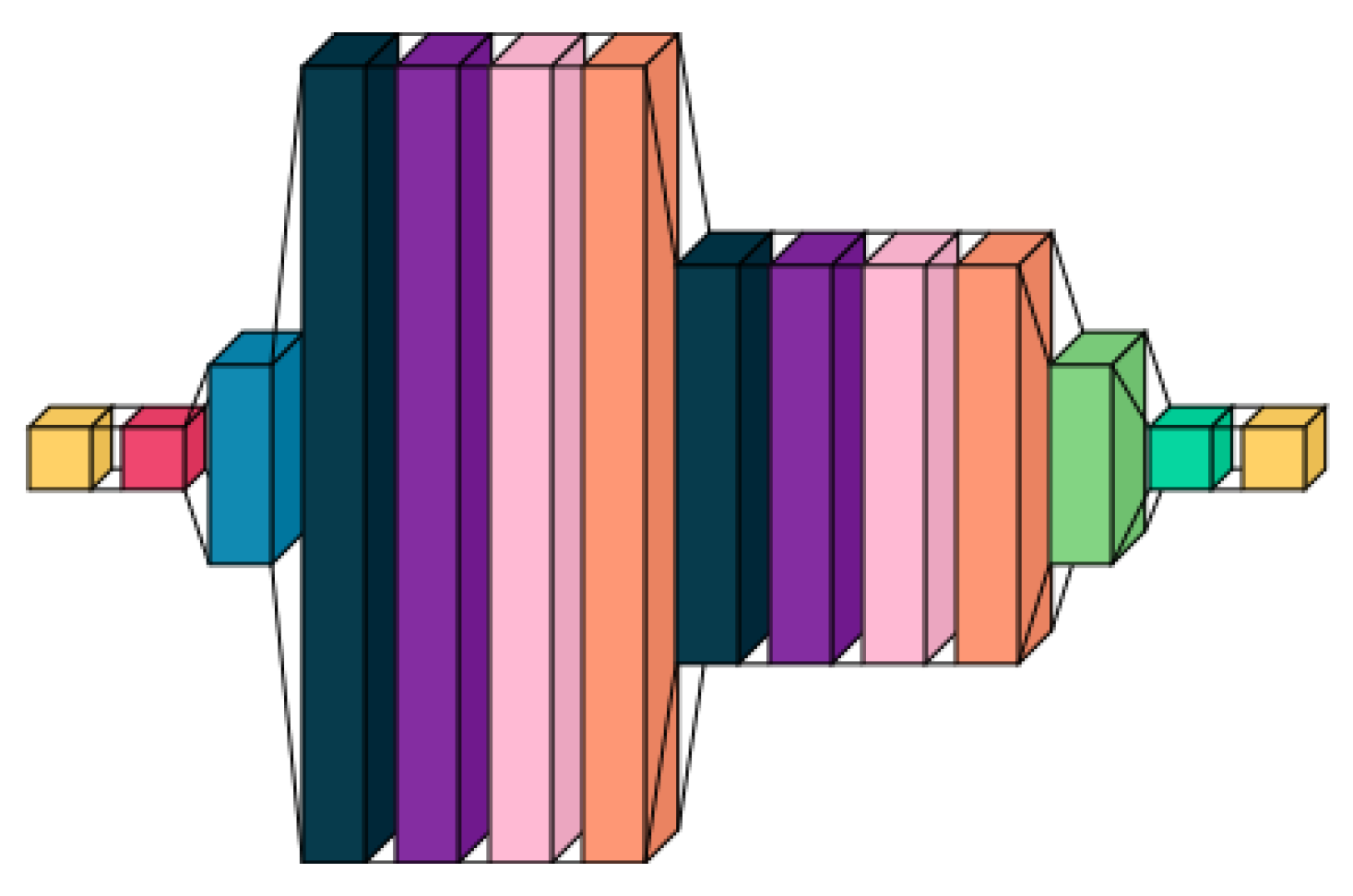
Our introduced malware detection framework utilizes a dense neural network (DNN) structure augmented with sophisticated deep learning methods to effectively and reliably detect malware. The system starts with two unique input layers: an auxiliary input layer that captures supplementary features such as metadata and file attributes, and another input layer for textual data that processes sequences of API calls or machine instructions. These sequences play a vital role in the recognition of malware through behavioral analysis. The neural network acts as a feature extractor, which is then followed by independent classifiers in distinct pipelines.
Input Processing
The input is indicated as (Very First Yellow Block) , with N representing the number of samples and F representing the number of features. This input goes through multiple dense layers. Following the initial dense layer, which consists of 52 units and uses a linear activation function, there is an additional dense layer with the same setup. Each dense layer is followed by a batch normalization layer to enhance the stability and speed of the training. Mathematically,
, where W and b represent the weights and biases of the dense layer, and denotes the activation function (ReLU). The batch normalization layer adjusts H to have a mean of 0 and a variance of 1, that is,
. ReLU activation functions are employed post-batch normalization to add nonlinearity, and dropout layers are included to mitigate overfitting.
- N: number of samples (individual files being analyzed)
- F: number of features extracted from each file
- : real number values
- W: weight matrix
- b: bias vector
- : activation function (ReLU)
- H: dense layer output
- : batch mean
- : batch variance
- : small constant for numerical stability
Attention Layer
The architecture incorporates a multi-head attention mechanism (The Dark Blue Block) to grasp long-term dependencies and contextual data. The self-attention can be formulated as:
where denotes the query, key, and value matrices, and is the dimensionality of the keys. The multi-head attention mechanism aggregates several self-attention heads.
- Q: Query matrix (learned representation of input)
- K: Key matrix (learned representation for matching)
- V: Value matrix (learned representation for output)
- : Dimension of key vectors
Custom Capsule Layer and Convolutional Layers
A specialized capsule layer manages spatial hierarchies and preserves spatial relationships ( The Prussian Blue and following 3 blocks). Calculate capsules from inputs : Convolutional layers identify local patterns and decrease spatial dimensions. The convolution operation is characterized as , where W denotes the filter, x represents the input, b is the bias and f is the activation function.
- : input vector to capsule
- : output vector
- : magnitude of input vector
LSTM Layers
LSTM layers ( The Medium Prussian Blue and following 3 blocks) manage different input sizes and timing patterns by capturing sequential dependencies:
- : input gate
- : forget gate
- : output gate
- : cell state
- : hidden state
- ⊙: element-wise multiplication
Feature Extraction and Classification Pipelines
The output of the neural network (The Light Green Block) is used as a feature extractor. This extracted feature set is then passed to different classification models using the Function Transformer to create separate pipelines:
Figure 1.
Feature Extraction Model.
Equations
A. Input Processing
- The input, denoted as , where N is the number of samples and F is the number of features, is processed through dense layers and batch normalization:where W and b are weights and biases of the dense layer, and is the activation function.
- Batch normalization:normalizes H to stabilize and accelerate training.
- N: number of samples (individual files being analyzed)
- F: number of features extracted from each file
- : real number values
- W: weight matrix
- b: bias vector
- : activation function (ReLU)
- H: dense layer output
- : batch mean
- : batch variance
- : small constant for numerical stability
B. Data Processing
- Global max pooling:reduces dimensionality while preserving important features.
C. Attention Layer
- The model incorporates a self-attention and Multi-Headed Attention layer to capture long-range dependencies:
- Self-attention:enhances focus on relevant parts of the input sequence.
- Multi-head attention:weighs different parts of the sequence differently.
- Q: Query matrix (learned representation of input)
- K: Key matrix (learned representation for matching)
- V: Value matrix (learned representation for output)
- : Dimension of key vectors
D. Capsule Layer
- A capsule layer maintains spatial relationships:preserves structure in the input data.
- : input vector to capsule
- : output vector
- : magnitude of input vector
E. LSTM Layers
- LSTM layers capture sequential dependencies:model sequential patterns and update state.
- : input gate
- : forget gate
- : output gate
- : cell state
- : hidden state
- ⊙: element-wise multiplication
F. Feature Extraction and Classification Pipelines
- The output features of the neural network:
- These features are then passed to different classifiers using Function Transformer to create separate pipelines:
Experimental Setup
The suggested method for identifying harmful files via machine learning utilizes a thorough and adaptable strategy applicable to all file formats. The main objective is to format the model as a binary classification task aimed at categorizing files as either malicious or benign (goodware). The dataset includes feature vectors gathered from different file types, where each vector signifies particular file characteristics, such as metadata, structure, content patterns, or other unique attributes.
The model’s architecture starts with an auxiliary input layer that handles these extracted feature vectors. Following this are dense (fully connected) layers, each integrated with batch normalization to standardize the activations. This approach ensures the training process is efficient and robust, reducing issues such as vanishing or exploding gradients. Incorporating ReLU (Rectified Linear Unit) activation functions introduces non-linearity, enabling the model to learn intricate and subtle patterns related to file behavior. To avoid overfitting, dropout layers are carefully positioned after the dense layers, randomly disabling a subset of neurons during each training cycle. This helps the model generalize better to new data, which is crucial given the natural variability of file types.
To better augment the model’s capacity to detect complex patterns in the data, the architecture incorporates a transformer encoder. This layer integrates an attention mechanism that allows the model to dynamically focus on various segments of the input sequence. The attention mechanism is especially proficient at identifying critical features that could signify malicious actions. The addition of global max pooling layers minimizes the data’s dimensionality by selecting the most pertinent features, whereas multi-head attention layers assist the model in capturing multiple facets of the data concurrently.
The model integrates convolutional operations via a Conv1D (1D Convolutional) layer, succeeded by a bespoke capsule layer. This capsule layer is essential for maintaining spatial hierarchies and feature relationships, enabling the model to comprehend the internal structures of files, which is often crucial for differentiating between malicious and benign files. The output from the capsule layer is flattened, allowing it to merge smoothly with the subsequent layers and aiding in the uninterrupted flow of information through the network.
Temporal sequences and changing patterns in file behaviors are captured with LSTM (Long Short-Term Memory) layers. These layers are essential for files where sequential data, like timestamped events or incremental actions, is crucial for detecting malicious activities. Additionally, graph layers are incorporated into the architecture to represent complex feature interactions. Often, the interrelation between various file attributes can suggest malicious intent, and graph-based models enhance the understanding of these connections.
To integrate the various features and representations acquired by different segments of the model, concatenation layers are implemented. These layers amalgamate the outputs from multiple sections of the model, guaranteeing a thorough and enriched final representation of the input. Additional dense layers, featuring batch normalization, ReLU activation, and dropout, further enhance and process these learned features before they are relayed to the final output layer.
The output layer has two units and leverages a softmax activation function to generate probabilistic outputs. These outputs indicate the chances of a file being either malicious or benign. Given that this is a binary classification task, softmax guarantees that the two probabilities add up to one, offering an interpretable outcome that can be used for classification by applying a threshold.
To train and evaluate, the model follows a supervised learning approach. The dataset is partitioned into three segments: train, validation, and test sets. The training subset is used to fit the model, whereas the validation subset assists in tuning hyperparameters and avoiding overfitting via early stopping. The test subset, which contains samples from diverse sources like private malware repositories, is kept for the ultimate model assessment.
To evaluate the model’s performance, four primary metrics are employed: accuracy, recall, F1-score, and ROC-AUC. Accuracy indicates the overall correctness of the model, whereas recall emphasizes the model’s capacity to accurately detect malicious files. The F1-score, which is the harmonic mean of precision and recall, provides a balanced perspective on the trade-off between false positives and false negatives, a critical aspect in malware detection. ROC-AUC assesses the model’s ability to differentiate between classes at various thresholds, providing insights into its discriminatory effectiveness.
Accuracy
The accuracy of the model is given by:
where:
- is the number of true positives (correctly classified malware),
- is the number of true negatives (correctly classified goodware),
- is the number of false positives (benign files incorrectly classified as malware),
- is the number of false negatives (malicious files incorrectly classified as benign).
Recall
Recall (or True Positive Rate) is given by:
This metric measures the model’s ability to correctly identify malware.
Precision
Precision is defined as:
This metric measures the proportion of true positives among all files predicted as malware.
F1-Score
The F1-Score, which balances precision and recall, is calculated as:
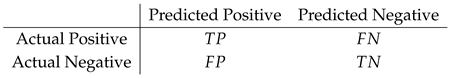
Finally, confusion matrices are utilized to analyze the distribution of true positives, true negatives, false positives, and false negatives. Since malware is treated as the positive class, the confusion matrix helps in understanding the occurrence of false positives and false negatives, allowing for targeted adjustments to minimize misclassifications. By combining neural network architectures with classical machine learning techniques such as Support Vector Machines, Random Forest, and Multilayer Perceptron, the framework offers a robust solution for detecting malicious files across a wide variety of file types.
Confusion Matrix
The confusion matrix helps visualize the performance of the classification model. For binary classification, the confusion matrix is defined as:
 where:
where:- (True Positive) is the number of correctly classified malware,
- (False Negative) is the number of malware incorrectly classified as benign,
- (False Positive) is the number of benign files incorrectly classified as malware,
- (True Negative) is the number of correctly classified benign files.
Results
Validation Results
In order to assess the performance of various machine learning algorithms, a validation phase was conducted. This phase involved testing Support Vector Machine (SVM), Random Forest (RF), and Multilayer Perceptron (MLP) algorithms over the validation dataset, with the goal of selecting the most promising models for the subsequent testing phase. The evaluation metrics used include Accuracy, Precision, Recall, F1-Score, and ROC-AUC.
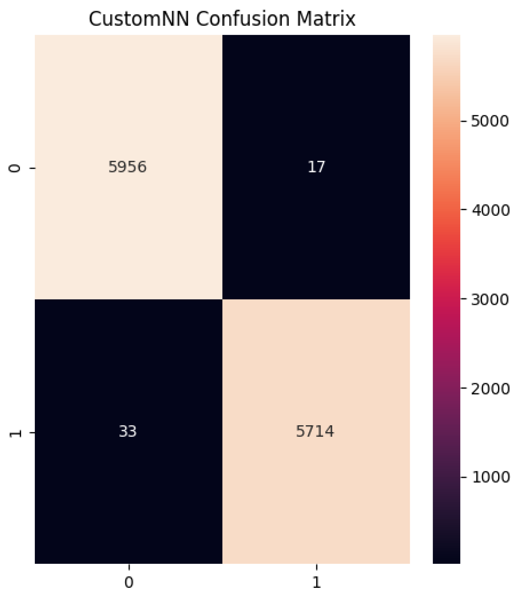
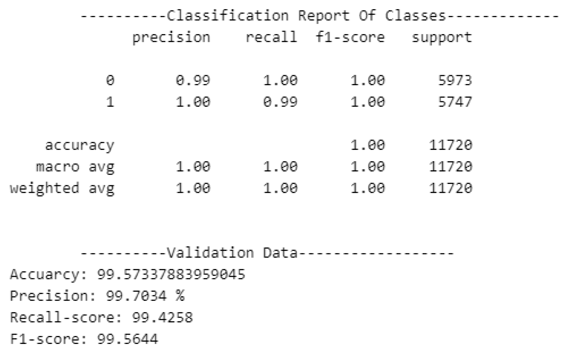
As shown in Figure 3, the Random Forest model produced outstanding results in the validation phase, achieving near-perfect accuracy, recall, and F1-scores. Notably, the system’s performance across classes (0 for goodware and 1 for malware) indicated excellent precision and recall values, suggesting that the RF classifier can detect malware efficiently with minimal false positives or false negatives.
The Random Forest achieved the highest precision (99.7034%), a recall score of 99.4258%, and an F1-Score of 99.5644%. These results surpass the SVM and even slightly outperform the MLP classifier, particularly in terms of precision. The metrics suggest that the Random Forest classifier is the most reliable for malware detection on the validation dataset.
Figure 3.
Classification Report for Random Forest in the Validation Phase.
Test Results
For the testing phase, a fresh set of malware samples was collected from private repositories, and goodware was obtained from the eDonkey/Kad network using eMule. This approach ensured that the dataset used in testing was entirely distinct from the training and validation datasets. By adopting different sources, the model’s performance in a real-world setting was emulated, with special attention given to the robustness of the system over time.
Performance metrics for the test phase reveal that the Support Vector Machine (SVM) algorithm’s performance drastically worsened when compared to the validation phase. This indicates that SVM is unsuitable for malware detection in this context. On the other hand, both Random Forest and Multilayer Perceptron exhibited excellent generalization, with MLP slightly outperforming Random Forest across several metrics, including False Positives and False Negatives.
Moreover, MLP slightly surpassed RF in terms of prediction time, making it more efficient in a practical setting. Given the high recall of both RF and MLP and the minimal False Negative rates, both classifiers are recommended for real-time malware detection. However, MLP’s superior handling of False Positives and marginally faster prediction times make it the more robust solution.

Table 1.
Performance comparison in test phase.
| Algorithm | Accuracy | Recall | F1-Score | ROC-AUC |
|---|---|---|---|---|
| MLP | 0.96 | 0.967 | 0.96 | 0.98 |
Conclusions
Utilizing dense neural networks, specialized capsule layers, and attention mechanisms, our architecture provides a robust method for malware detection. It adeptly identifies both local and global patterns, differentiating between benign and harmful files, even in adversarial situations. The neural network acts as a feature extractor, and through a Function Transformer, we develop distinct pipelines where the neural network is shared across all pipelines, with other models in the pipeline including Random Forest, Decision Tree, Logistic Regression, and Gaussian Naive Bayes.
Future Work
To improve the accuracy of the project, it is crucial to invest time in recreating an enterprise environment for dependable data collection and practical testing. Furthermore, exploring the training of multi-attention head transformers for URL detection, modifying the model for other forms of malicious threats or creating new models, acquiring and retraining the model with larger datasets, enhancing the prevention engine to generate more dynamic rule outputs, and integrating real-time prevention mechanisms via host-based network monitors are important steps.
References
- Nataraj, L.; Karthikeyan, S.; Jacob, G.; Manjunath, B. Malware images: Visualization and automatic classification. Proceedings of the 8th International Symposium on Visualization for Cyber Security 2011. [Google Scholar] [CrossRef]
- Vasan, D.; Alazab, M.; Safaei, B. Image-based malware classification using convolutional neural networks. Journal of Computer Virology and Hacking Techniques 2020, 16, 283–297. [Google Scholar]
- Ferrag, M.A.; Maglaras, L.; Moschoyiannis, S.; Janicke, H. Deep learning for cyber security intrusion detection: Approaches, datasets, and comparative study. Journal of Information Security and Applications 2020, 50, 102419. [Google Scholar] [CrossRef]
- Wang, X.; Zhao, Y.; Liang, Y. A bibliometric analysis of deep learning for malware detection research. IEEE Access 2018, 6, 33311–33321. [Google Scholar]
- Gharibian, S.; Ghorbani, A.A. A comparison of machine learning and deep learning approaches for malware detection. Security and Privacy Journal 2015. [Google Scholar]
- Hou, X.; Zhou, C.; Duan, L. A categorization of deep learning-based methods for malware detection. Journal of Computer Virology and Hacking Techniques 2016. [Google Scholar]
- Ye, Y.; Wang, D.; Li, T. Hybrid deep learning models for malware detection. IEEE Transactions on Information Forensics and Security 2019, 15, 3265–3277. [Google Scholar]
- Saxe, J.; Berlin, K. Deep neural network-based malware classification using binary file representations. Proceedings of the 10th International Conference on Malicious and Unwanted Software 2015. [Google Scholar] [CrossRef]
- Huang, L.; Stokes, J.W. Long short-term memory networks for dynamic malware analysis. Proceedings of the 25th USENIX Security Symposium 2016. [Google Scholar]
- Shahriar, H.; Klintic, G. Dynamic analysis of evasive malware using RNNs. Journal of Cyber Security 2016. [Google Scholar]
- Al-Qatf, M.; Lasheng, Y.; Mohamad, N. Deep learning approach for malware detection in IoT systems. Future Generation Computer Systems 2018, 91, 91–98. [Google Scholar]
- Jin, Z.; Yan, C.; Yue, J. Towards unsupervised anomaly detection in malware detection. Computers & Security 2018, 75, 14–29. [Google Scholar]
- Kumar, A.; Chen, Y. Detecting malware using generative adversarial networks. IEEE Symposium on Security and Privacy 2017. [Google Scholar]
- David, O.; Netanyahu, N.S. Deep learning for detecting malware. Proceedings of the 28th IEEE Computer Security Foundations Symposium 2015. [Google Scholar]
- Kim, H.; Lee, D. Static malware detection using memory-efficient CNNs. IEEE Transactions on Cybernetics 2020. [Google Scholar]
- Siddiqui, S.; Qureshi, M.F. A lightweight deep learning framework for mobile malware detection. Journal of Mobile Networks and Applications 2019, 24, 1023–1032. [Google Scholar]
- Al-Garadi, M.A.; Mohammed, A.; Guizani, M. A survey on deep learning techniques in cybersecurity and malware detection. IEEE Communications Surveys & Tutorials 2020, 22, 1940–1971. [Google Scholar]
- Pham, Q.; Yun, I.D. Hybrid CNN-LSTM model for malware detection. Proceedings of the IEEE Conference on Computer Vision and Pattern Recognition 2017. [Google Scholar]
- Tobiyama, S.; Yamada, H. Dynamic malware behavior analysis using attention-based LSTM. Proceedings of the 33rd Annual Computer Security Applications Conference 2016. [Google Scholar]
- Luo, X.; Yan, J. Automatic feature extraction for malware detection. Journal of Cyber Security Technology 2017, 1, 123–134. [Google Scholar]
- Xu, T.; Wang, P.; Liu, B. Enhancing malware detection with graph neural networks. IEEE Transactions on Neural Networks and Learning Systems 2020. [Google Scholar]
- Li, F.; Zhang, P. Learning adaptive malware detection models using reinforcement learning. Proceedings of the 14th ACM ASIA Conference on Computer and Communications Security 2018. [Google Scholar]
- Zhao, Y.; Qin, J. A dynamic deep learning model for malware detection. IEEE Access 2019, 7, 54543–54554. [Google Scholar]
- Sung, E.; Kim, D.S. Multi-task learning for detecting multiple malware families. Security and Privacy in Computing Systems 2016, 10–18. [Google Scholar]
- Zhou, X.; Xiao, X. Deep ensemble model for malware detection across multiple vectors. IEEE Access 2018, 6, 70571–70580. [Google Scholar]
- Berman, R.; Weck, R. Adversarial resilience in malware detection using deep learning. IEEE Transactions on Information Forensics and Security 2020. [Google Scholar]
- Wu, J.; Zhang, X. A survey on convolutional neural networks in cybersecurity. Journal of Cyber Security 2017, 42, 116–130. [Google Scholar]
- Pektas, A.; Acarman, T. Hybrid CNN-GRU architecture for malware detection. IEEE Transactions on Cybernetics 2018. [Google Scholar]
- Zhang, H.; Chen, K. Detection of malware using transfer learning. IEEE Transactions on Big Data 2019. [Google Scholar]
- Chen, J.; Wu, Y. An end-to-end deep learning approach for malware classification. IEEE Access 2020, 8, 1234–1245. [Google Scholar]
Figure 2.
Classification Report for Random Forest in the Validation Phase.
Disclaimer/Publisher’s Note: The statements, opinions and data contained in all publications are solely those of the individual author(s) and contributor(s) and not of MDPI and/or the editor(s). MDPI and/or the editor(s) disclaim responsibility for any injury to people or property resulting from any ideas, methods, instructions or products referred to in the content. |
© 2025 by the authors. Licensee MDPI, Basel, Switzerland. This article is an open access article distributed under the terms and conditions of the Creative Commons Attribution (CC BY) license (http://creativecommons.org/licenses/by/4.0/).
Copyright: This open access article is published under a Creative Commons CC BY 4.0 license, which permit the free download, distribution, and reuse, provided that the author and preprint are cited in any reuse.


