Submitted:
23 January 2025
Posted:
24 January 2025
You are already at the latest version
Abstract
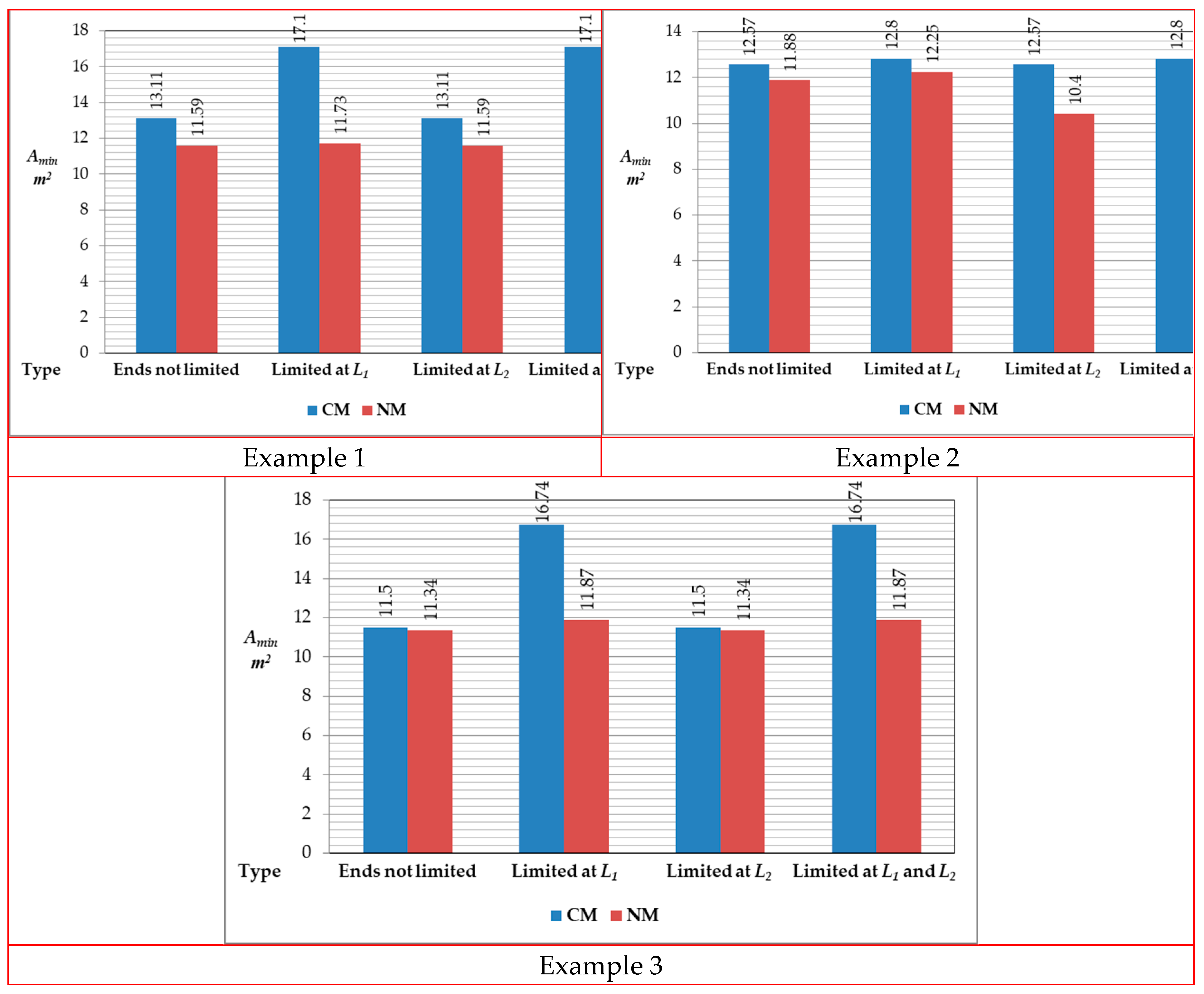
This study shows an optimal model to obtain the minimum contact surface with the ground for T-shaped combined footings, taking into account that the surface works partially under compression, this is, a part of the surface under the footing in contact with the ground is under compression and the other part the pressure is zero (linear pressure on the ground). There are works that show the minimum surface for T-shaped combined footings, but the surface beneath the footing in contact with the ground works entirely in compression. The model is developed by integration and/or by the geometric properties of a pyramid with a triangular-based to obtain the equations of the resultant force and the two moments (X and Y axes) for the fifteen cases of biaxial bending and three special cases of uniaxial bending (My1 and My2 are equals to zero). Three numerical examples are presented with the same data: Example 1 is for different bending moments; Example 2 is for bending moments Mx1 and Mx2 equals to zero; Example 3 is for bending moments My1 and My2 equals to zero. Also, a comparison is made with the current model (area works completely under compression) and the new model (area works partially under compression). The results show that savings of up to 31.40% can be achieved in the area of contact with the ground. In this way, the minimum surface model will be of great help to foundation engineering specialists.
Keywords:
MSC: 32A40; 51E99; 90C90
1. Introduction
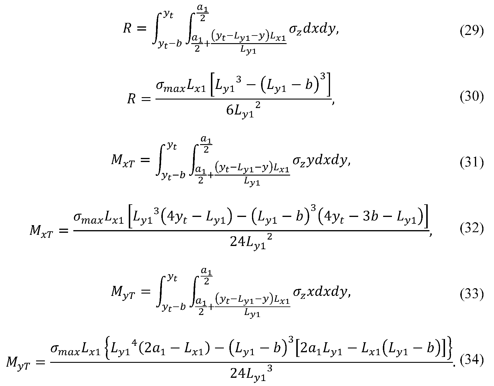
2. Formulation of the Model
2.1. Biaxial Bending
2.1.1. Case I
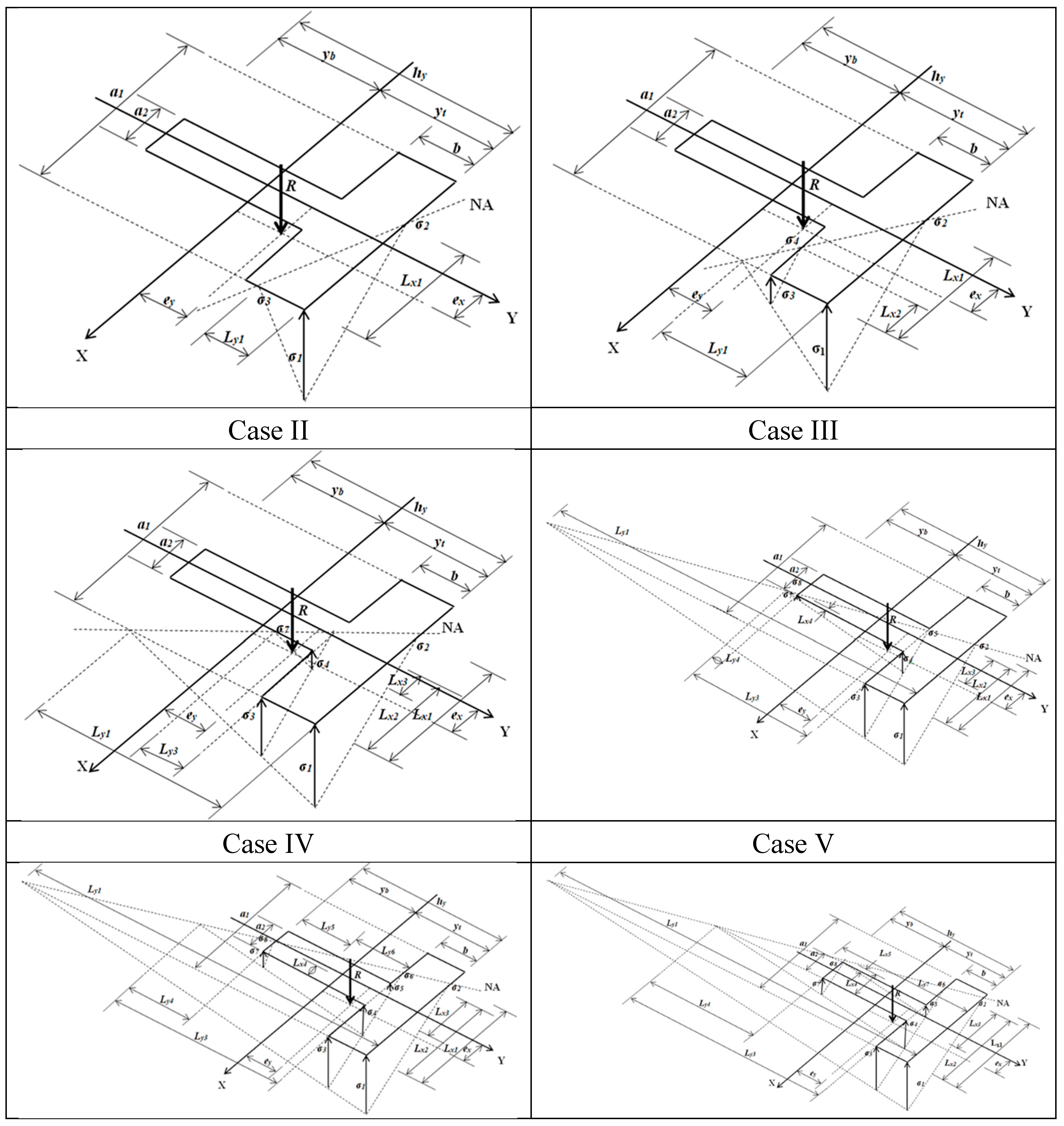
2.1.2. Case II
2.1.3. Case III
2.1.4. Case IV
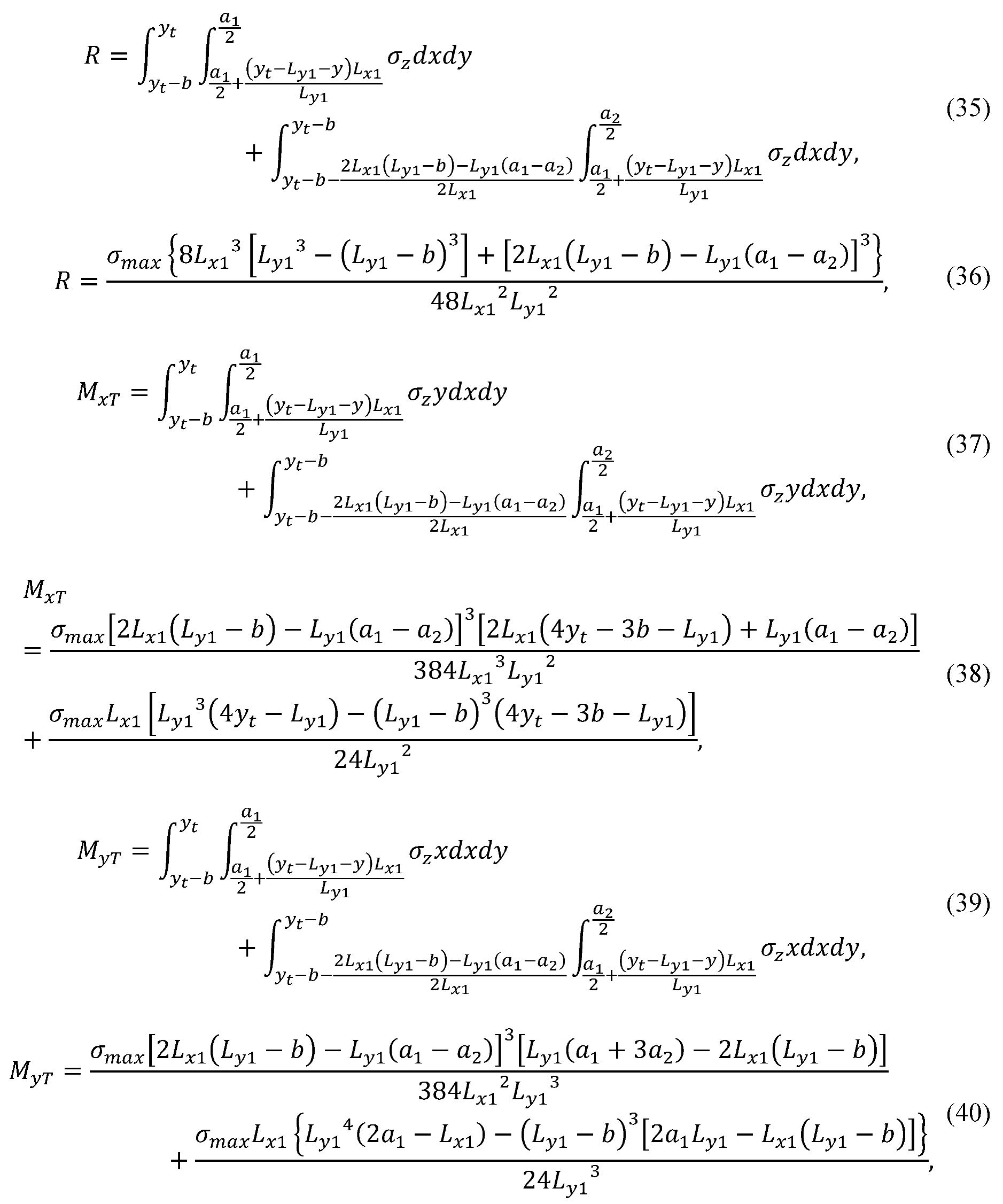
2.1.5. Case V
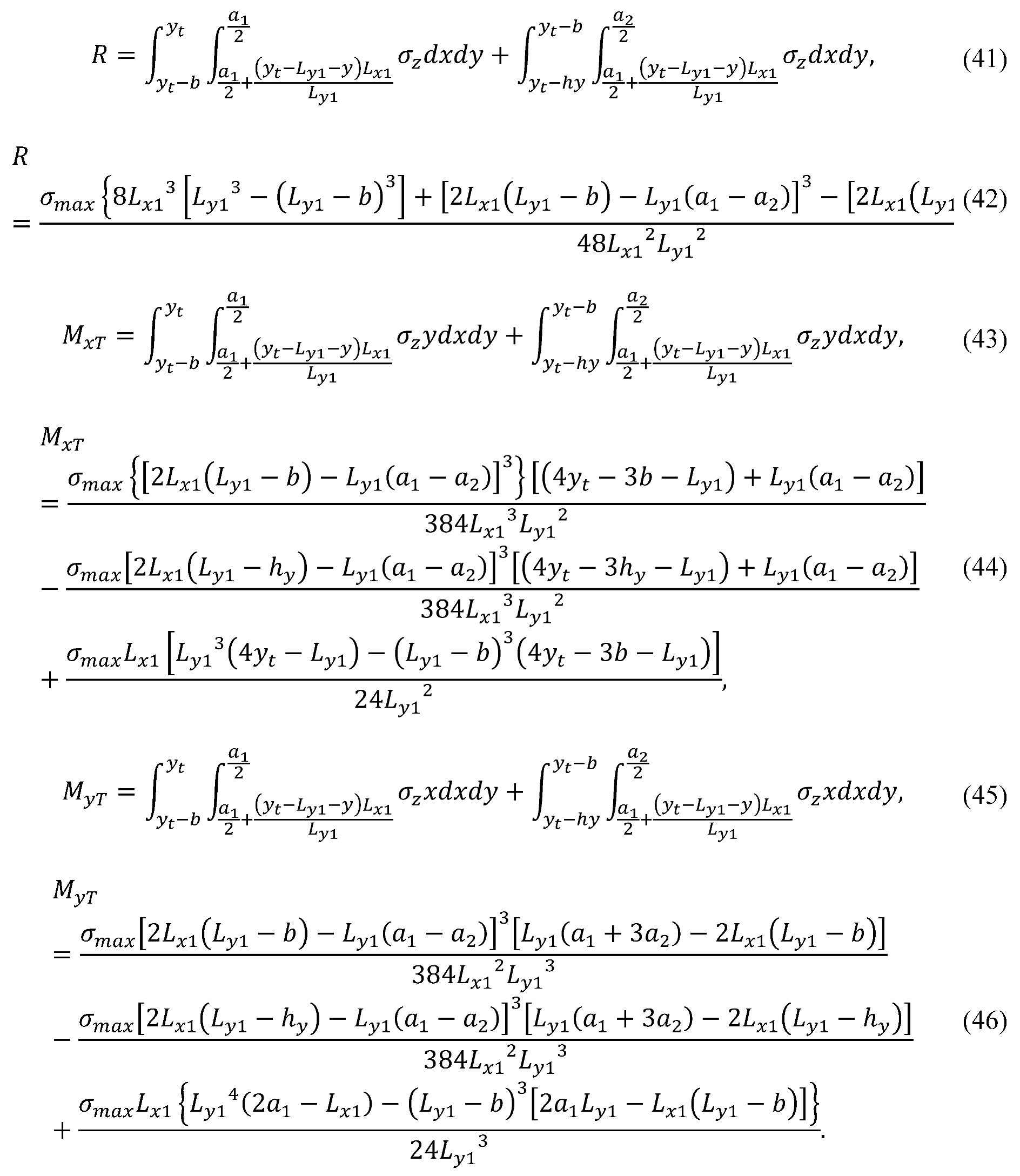
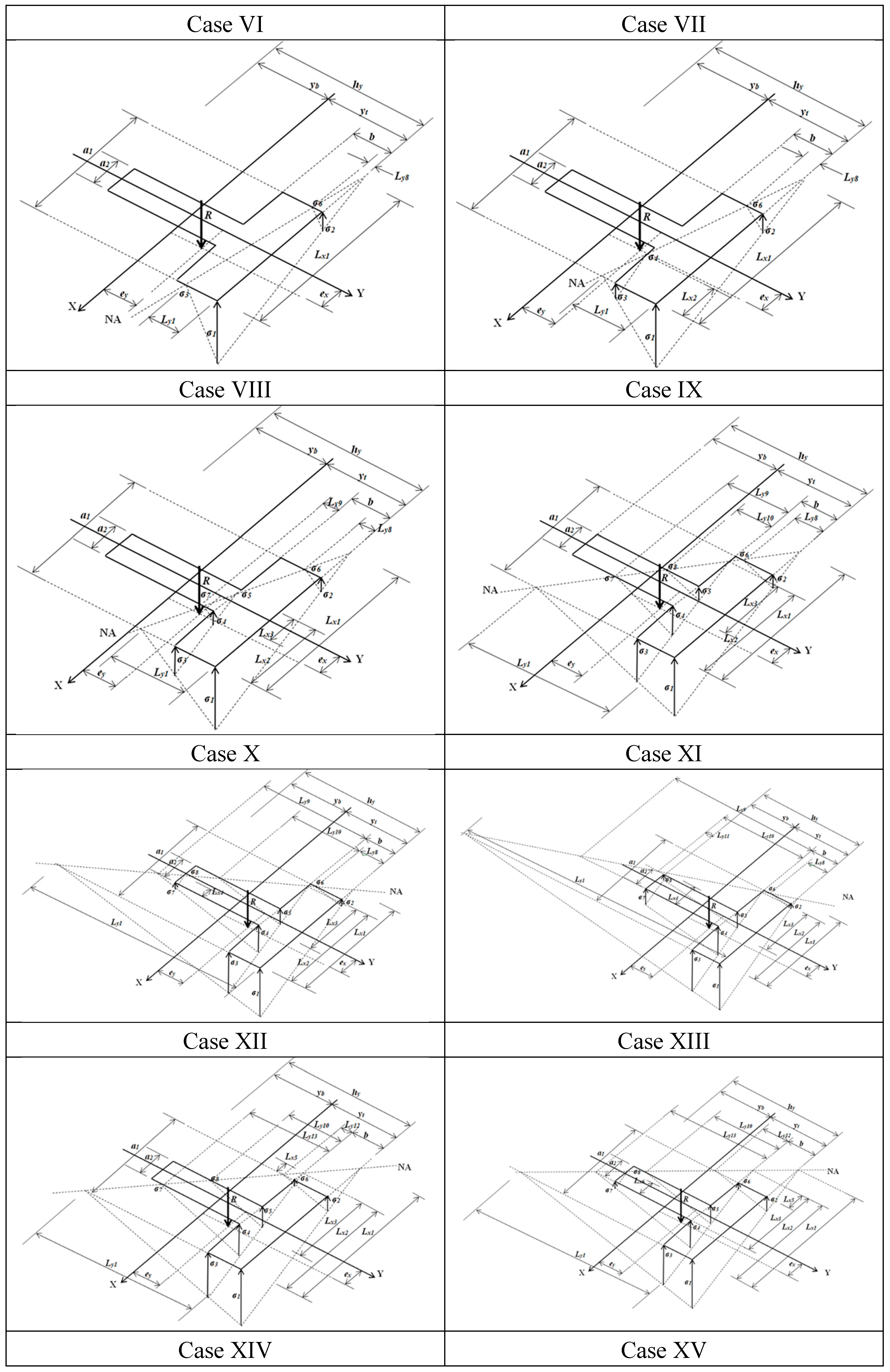
2.1.6. Case VI
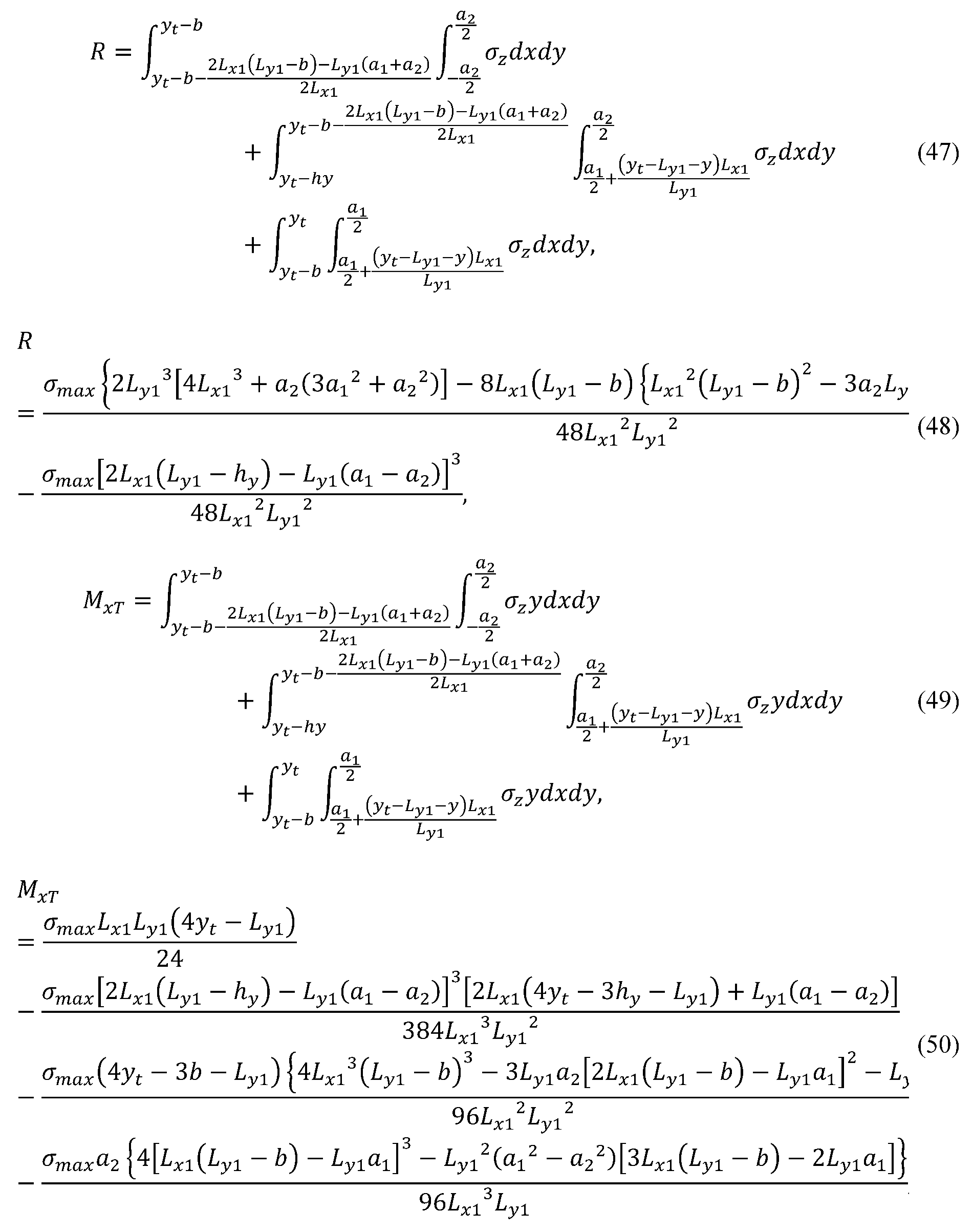
2.1.7. Case VII
2.1.8. Case VIII
2.1.9. Case IX
2.1.10. Case X
2.1.11. Case XI
2.1.12. Case XII
2.1.13. Case XIII
2.1.14. Case XIV
2.1.15. Case XV
2.2. Special Cases
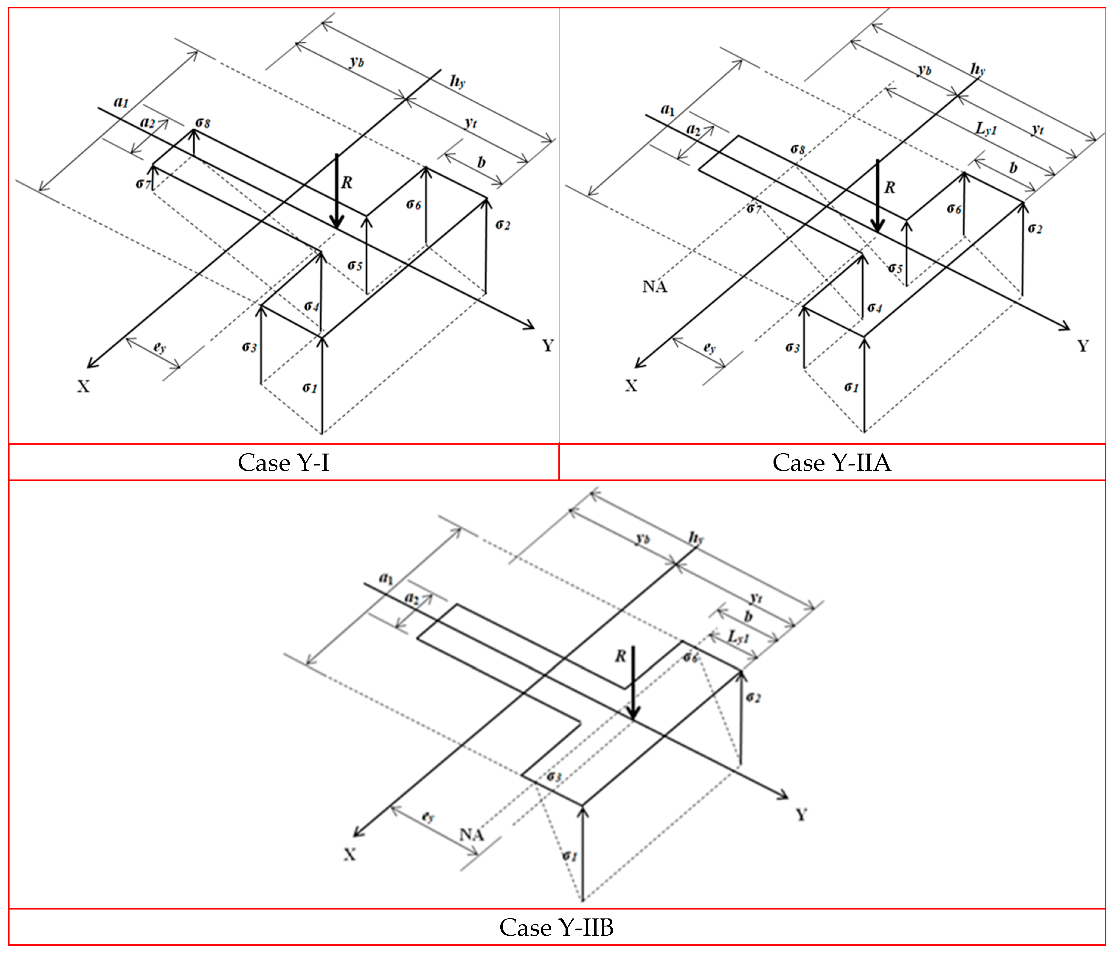
2.2.1. Case Y
2.2.2. Case X
2.3. Minimum Surface for T-Shaped Combined Footings
3. Numerical Examples
4. Results
5. Conclusions
Author Contributions
Funding
Data Availability Statement
Acknowledgments
Conflicts of Interest
References
- Bowles, J.E. Foundation analysis and design; McGraw-Hill, New York, USA, 2001.
- Shahin, M.A.; Cheung, E.M. Stochastic design charts for bearing capacity of strip footings. Geomech. Eng. 2011, 3, 153-167. [CrossRef]
- Dixit, M.S.; Patil K.A. Experimental estimate of Nγ values and corresponding settlements for square footings on finite layer of sand. Geomech. Eng. 2013, 5, 363-377. [CrossRef]
- ErzÍn, Y.; Gul, T.O. The use of neural networks for the prediction of the settlement of pad footings on cohesionless soils based on standard penetration test. Geomech. Eng. 2013, 5, 541-564. [CrossRef]
- Colmenares, J.E.; Kang, S-R.; Shin, Y-J.; Shin, J-H. Ultimate bearing capacity of conical shell foundations. Struct. Eng. Mech. 2014, 52, 507-523. [CrossRef]
- Cure, E.; Sadoglu, E.; Turker, E.; Uzuner, B.A. Decrease trends of ultimate loads of eccentrically loaded model strip footings close to a slope. Geomech. Eng. 2014, 6, 469-485. [CrossRef]
- Fattah, M.Y.; Yousif, M.A.; Al-Tameemi, S.M.K. Effect of pile group geometry on bearing capacity of piled raft foundations”, Struct. Eng. Mech. 2015, 54, 829-853. [CrossRef]
- Uncuoğlu, E. The bearing capacity of square footings on a sand layer overlying clay”, Geomech. Eng. 2015, 9, 287-311. [CrossRef]
- Anil, Ö.; Akbaş, S.O.; BabagĪray, S.; Gel, A.C.; Durucan, C. Experimental and finite element analyses of footings of varying shapes on sand”, Geomech. Eng. 2017, 12, 223-238. [CrossRef]
- Khatri, V.N.; Debbarma, S.P.; Dutta, R.K.; Mohanty, B. Pressure-settlement behavior of square and rectangular skirted footings resting on sand. Geomech. Eng. 2017, 12, 689-705. [CrossRef]
- Mohebkhah, A. Bearing capacity of strip footings on a stone masonry trench in clay. Geomech. Eng. 2017, 13, 255-267. [CrossRef]
- Zhang, W.-X.; Wu, H.; Hwang, H.-J.; Zhang, J.-Y.; Chen, B.; Yi, W.-J. Bearing behavior of reinforced concrete column-isolated footing substructures. Eng. Struct. 2019, 200, 109744. [CrossRef]
- Turedi, Y.; Emirler, B.; Ornek, M.; Yildiz, A. Determination of the bearing capacity of model ring footings: Experimental and numerical investigations. Geomech. Eng. 2019, 18, 29-39. [CrossRef]
- Gnananandarao, T.; Khatri, V.N.; Dutta, R.K. Bearing capacity and settlement prediction of multi-edge skirted footings resting onsand. Ing. Investig. 2020, 40, 9-21. [CrossRef]
- Gör, M. Analyzing the bearing capacity of shallow foundations on two-layered soil using two novel cosmology-based optimization techniques. Smart Struct. Syst. 2022, 29, 513-522. [CrossRef]
- Chaabani, W.; Remadna, M.S.; Abu-Farsakh, M. Numerical Modeling of the Ultimate Bearing Capacity of Strip Footings on Reinforced Sand Layer Overlying Clay with Voids. Infrastructures 2023, 8, 3. [CrossRef]
- Vitone, D.M.A.; Valsangkar, A.J. Stresses from loads over rectangular areas. J. Geotech. Geoenviron. 1986, 112, 961-964. [CrossRef]
- Michalowski, R.L. Upper-bound load estimates on square and rectangular footings. Géotechnique. 2001, 51, 787-798. [CrossRef]
- Özmen, G. Determination of base stresses in rectangular footings under biaxial bending. Teknik Dergi Digest. 2011, 22, 1519-1535. http://www.imo.org.tr/resimler/dosya_ekler/7b559795bd3f63b_ek.pdf?dergi=472.
- Aydogdu, I. New Iterative method to Calculate Base Stress of Footings under Biaxial Bending. IJEAS. 2016, 8, 40-48. [CrossRef]
- Girgin, K. Simplified formulations for the determination of rotational spring constants in rigid spread footings resting on tensionless soil. JCEM. 2017, 23, 464-474. [CrossRef]
- Al-Gahtani, H.J.; Adekunle, S.K. A boundary-type approach for the computation of vertical stresses in soil due to arbitrarily shaped foundations. World J. Eng. 2019, 16, 419-426. [CrossRef]
- Rawat, S.; Mittal, R.K.; Muthukumar, G. Isolated Rectangular Footings under Biaxial Bending: A Critical Appraisal and Simplified Analysis Methodology. Pract. Period. Struct. Des. Const. 2020, 25. [CrossRef]
- López-Machado, N.A.; Perez, G.; Castro, C.; Perez, J.C.V.; López-Machado, L.J.; Alviar-Malabet, J.D.; Romero-Romero, C.A.; Guerrero-Cuasapaz, D.P.; Montesinos-Machado, V.V. A Structural Design Comparison Between Two Reinforced Concrete Regular 6-Level Buildings using Soil-Structure Interaction in Linear Range. Ing. Investig. 2022, 42, e86819. [CrossRef]
- Lezgy-Nazargah, M.; Mamazizi, A.; Khosravi, H. Analysis of shallow footings rested on tensionless foundations using a mixed finite element model. Struct. Eng. Mech. 2022, 81, 379-394. [CrossRef]
- Teng, W.C. Foundation Design; Prentice-Hall Inc.: New Delhi, India, 1979.
- Highter, W.H.; Anders, J.C. Dimensioning footings subjected to eccentric loads. J. Geotech. Geoenviron. 1985, 111, 659-665. [CrossRef]
- Galvis, F.A.; Smith-Pardo, P.J. Axial load biaxial moment interaction (PMM) diagrams for shallow foundations: Design aids, experimental verification, and examples. Eng. Struct. 2020, 213, 110582. [CrossRef]
- Rodriguez-Gutierrez, J.A.; Aristizabal-Ochoa, J.D. Rigid spread footings resting on soil subjected to axial load and biaxial bending. I: Simplified analytical method. Int. J. Geomech. 2013, 13, 109-119. [CrossRef]
- Rodriguez-Gutierrez, J.A.; Aristizabal-Ochoa, J.D. Rigid spread footings resting on soil subjected to axial load and biaxial bending. II: Design aids. Int. J. Geomech. 2013, 13, 120-131. [CrossRef]
- Maheshwari, P.; Khatri, S. Influence of inclusion of geosynthetic layer on response of combined footings on stone column reinforced earth beds. Geomech. Eng. 2012, 4, 263-279. [CrossRef]
- Konapure, C.G.; Vivek, B. Analysis of Combined rectangular footing by Winkler’s Model and Finite Element Method. International JEIT. 2013, 3, 128-132. https://www.ijeit.com/Vol%203/Issue%205/IJEIT1412201311_21.pdf.
- Vivek, B.; Arkal, L.S.; Bandgar, R.V.; Kalekhan, F.A.S. Comparative Study on Conventional and Simplified Elastic Analysis of Rectangular Combined Footing. Int. J. Res. Eng. Technol.,¿ 2014, 3, 422-427. https://ijret.org/volumes/2014v03/i04/IJRET20140304076.pdf.
- Ravi Kumar Reddy, C.; Satish Kumar, M.; Kondala Rao, M.; Gopika, N. Numerical Analysis of Rectangular Combined Footings Resting on Soil for Contact Pressure. Int. J. Civil Engi. Technol. 2018, 9, 1425-1431. http://iaeme.com/Home/issue/IJCIET?Volume=9&Issue=9.
- Kashani, A.R.; Camp, C.V.; Akhani, M.; Ebrahimi, S. Optimum design of combined footings using swarm intelligence-based algorithms. Adv. Eng. Soft. 2022, 169, 103140. [CrossRef]
- Al-Douri, E.M.F. Optimum design of trapezoidal combined footings. Tikrit J. Eng. Sci. 2007, 14, 85–115. [CrossRef]
- Luévanos-Rojas, A. Optimization for trapezoidal combined footings: Optimal design. Adv. Concrete Constr., Int. J. 2023, 16, 21-34. [CrossRef]
- Luévanos-Rojas, A.; López-Chavarría, S.; Medina-Elizondo, M. A new model for T-shaped combined footings Part I: Optimal dimensioning. Geomech. Eng. 2018, 14, 51-60. [CrossRef]
- Luévanos-Rojas, A.; López-Chavarría, S.; Medina-Elizondo, M. A new model for T-shaped combined footings Part II: Mathematical model for design. Geomech. Eng. 2018, 14, 61-69. http://dx.doi.org/10.12989/gae.2018.14.1.061.
- Moreno-Landeros, V.M.; Luévanos-Rojas, A.; SantiagoHurtado, G.; López-León, L.D.; Olguin-Coca, F.J.; López-León, A.L.; Landa-Gómez, A.E. Optimal Cost Design of RC T-Shaped Combined Footings. Buildings 2024, 14, 3688. [CrossRef]
- Aishwarya, K.M.; Balaji, N.C. Analysis and design of eccentrically loaded corner combined footing for rectangular columns. International Conference on Advances in Sustainable Construction Materials, Guntur, India, 18-19 March 2022. [CrossRef]
- Luévanos-Rojas, A.; Santiago-Hurtado, G.; Moreno-Landeros, V.M.; Olguin-Coca, F.J.; López-León, L.D.; Diaz-Gurrola, E.R. Mathematical Modeling of the Optimal Cost for the Design of Strap Combined Footings. Mathematics 2024, 12, 294. [CrossRef]

| Case | Equations |
| I | Equations (1) to (5), (7) to (9), (15) to (22), 0 ≤ σ1 to σ8 ≤ σmax |
| II | Equations (1), (2), (7) to (9), (24), (26), (28), Ly1 ≤ b, Lx1 ≤ a1 |
| III | Equations (1), (2), (7) to (9), (30), (32), (34), Ly1 ≥ b, Lx1 ≤ a1 |
| IV | Equations (1), (2), (7) to (9), (36), (38), (40), Ly1 ≥ b, Lx1 ≤ a1 |
| V | Equations (1), (2), (7) to (9), (42), (44), (46), Ly1 ≥ hy, Lx1 ≤ a1 |
| VI | Equations (1), (2), (7) to (9), (48), (50), (52), Ly1 ≥ hy, Lx1 ≤ a1 |
| VII | Equations (1), (2), (7) to (9), (54), (56), (58), Ly1 ≥ hy, Lx1 ≤ a1 |
| VIII | Equations (1), (2), (7) to (9), (60), (62), (64), Ly1 ≤ b, Lx1 ≥ a1 |
| IX | Equations (1), (2), (7) to (9), (66), (68), (70), Ly1 ≥ b, Lx1 ≥ a1 |
| X | Equations (1), (2), (7) to (9), (72), (74), (76), Ly1 ≥ b, Lx1 ≥ a1 |
| XI | Equations (1), (2), (7) to (9), (78), (80), (82), Ly1 ≥ b, Lx1 ≥ a1 |
| XII | Equations (1), (2), (7) to (9), (84), (86), (88), Ly1 ≥ b, Lx1 ≥ a1 |
| XIII | Equations (1), (2), (7) to (9), (90), (92), (94), Ly1 ≥ b, Lx1 ≥ a1 |
| XIV | Equations (1), (2), (7) to (9), (96), (98), (100), Ly1 ≥ b, Lx1 ≥ a1 |
| XV | Equations (1), (2), (7) to (9), (102), (104), (106), Ly1 ≥ b, Lx1 ≥ a1 |
| Case | Equations |
| Y-I | Equations (1) to (5), (7) to (9), (15) to (22), 0 ≤ σ1 to σ8 ≤ σmax |
| Y-IIA | Equations (1), (2), (7) to (9), (111) to (113), Ly1 ≥ b, Ly1 ≤ hy |
| Y-IIB | Equations (1), (2), (7) to (9), (115) to (117), Ly1 ≤ b |
| Case |
Amin m2 |
|||
| Ends not limited | Limited at L1 | Limited at L2 | Limited at L1 and L2 | |
| I | 13.11 | 17.10 | 13.11 | 17.10 |
| II | 45.00 | * | * | * |
| III | 15.85 | * | 15.85 | * |
| IV | 21.93 | * | * | * |
| V | 15.62 | * | 15.62 | * |
| VI | 11.59 | 11.73 | 11.59 | 15.51 |
| VII | 15.53 | * | 15.53 | * |
| VIII | 23.45 | 22.36 | 23.45 | 22.36 |
| IX | 12.61 | 16.78 | 12.61 | 16.78 |
| X | 14.09 | 14.46 | 14.09 | 14.46 |
| XI | 12.98 | 16.58 | 12.98 | 16.58 |
| XII | 14.94 | * | 14.94 | * |
| XIII | 12.88 | 16.46 | 12.88 | 16.46 |
| XIV | 13.12 | 13.44 | 13.12 | 13.44 |
| XV | 12.71 | * | 12.71 | * |
| Case |
Amin m2 |
|||
| Ends not limited | Limited at L1 | Limited at L2 | Limited at L1 and L2 | |
| I | 12.57 | 12.80 | 12.57 | 12.80 |
| II | 45.00 | * | * | * |
| III | 15.55 | * | 15.53 | * |
| IV | 21.91 | * | * | * |
| V | 15.26 | * | 15.26 | * |
| VI | 15.37 | 12.25 | 12.90 | 12.90 |
| VII | 15.06 | * | 15.05 | * |
| VIII | 22.45 | 22.45 | 22.45 | 22.45 |
| IX | 12.56 | 15.82 | 12.56 | 15.82 |
| X | 13.61 | 13.79 | 13.61 | 13.79 |
| XI | 15.66 | 15.48 | 10.40 | 15.48 |
| XII | 13.15 | * | 13.51 | * |
| XIII | 12.56 | 15.45 | 12.56 | 15.45 |
| XIV | 12.68 | 12.82 | 12.68 | 12.82 |
| XV | 11.88 | 12.78 | 11.14 | 12.16 |
| Case |
Amin m2 |
|||
| Ends not limited | Limited at L1 | Limited at L2 | Limited at L1 and L2 | |
| YI | 11.50 | 16.74 | 11.50 | 16.74 |
| YIIA | 11.34 | 11.87 | 11.34 | 11.87 |
| YIIB | 15.00 | 18.70 | 15.00 | 18.70 |
| Case |
R kN |
MxT kN-m |
MyT kN-m |
L1 m |
L2 m |
Lx1 m |
Ly1 m |
a1 m |
a2 m |
b m |
hy m |
yt m |
Amin m2 |
| Ends not limited | |||||||||||||
| VI | 1500 | 2034.12 | 400 | 0.20 | 0.20 | 0.92 | 6.40 | 3.38 | 1.00 | 2.18 | 6.40 | 2.26 | 11.59 |
| Limited footing at L1 | |||||||||||||
| VI | 1500 | 2663.63 | 400 | 0.20 | 1.19 | 0.92 | 7.39 | 3.32 | 1.00 | 1.87 | 7.39 | 2.68 | 11.73 |
| Limited footing at L2 | |||||||||||||
| VI | 1500 | 2034.12 | 400 | 0.20 | 0.20 | 0.92 | 6.40 | 3.38 | 1.00 | 2.18 | 6.40 | 2.26 | 11.59 |
| Limited footing at L1 and L2 | |||||||||||||
| XIV | 1500 | 1328.82 | 400 | 0.20 | 0.20 | 21.83 | 6.83 | 8.04 | 1.00 | 1.00 | 6.40 | 1.79 | 13.44 |
| Case |
R kN |
MxT kN-m |
MyT kN-m |
L1 m |
L2 m |
Lx1 m |
Ly1 m |
a1 m |
a2 m |
b m |
hy m |
yt m |
Amin m2 |
| Ends not limited | |||||||||||||
| XV | 1500 | 1095.78 | 400 | 0.25 | 0.20 | 50.00 | 5.54 | 6.44 | 1.00 | 1.00 | 6.45 | 1.98 | 11.88 |
| Limited footing at L1 | |||||||||||||
| VI | 1500 | 4437.68 | 400 | 0.20 | 3.78 | 0.92 | 9.98 | 3.27 | 1.00 | 1.00 | 9.98 | 4.16 | 12.25 |
| Limited footing at L2 | |||||||||||||
| XI | 1500 | 0 | 400 | 4.20 | 0.20 | 8.40 | 20.05 | 1.00 | 1.00 | 10.40 | 10.40 | 5.20 | 10.40 |
| Limited footing at L1 and L2 | |||||||||||||
| XV | 1500 | 1081.82 | 400 | 0.20 | 0.20 | 38.73 | 5.50 | 6.76 | 1.00 | 1.00 | 6.40 | 1.92 | 12.16 |
| Case |
R kN |
MxT kN-m |
MyT kN-m |
L1 m |
L2 m |
Ly1 m |
a1 m |
a2 m |
b m |
hy m |
yt m |
Amin m2 |
| Ends not limited | ||||||||||||
| YIIA | 1500 | 1476.28 | 0 | 0.50 | 0.20 | 6.44 | 5.64 | 1.00 | 1.00 | 6.70 | 2.18 | 11.34 |
| Limited footing at L1 | ||||||||||||
| YIIA | 1500 | 1582.81 | 0 | 0.20 | 0.20 | 5.12 | 6.47 | 1.00 | 1.00 | 6.40 | 1.96 | 11.87 |
| Limited footing at L2 | ||||||||||||
| YIIA | 1500 | 1476.28 | 0 | 0.50 | 0.20 | 6.44 | 5.64 | 1.00 | 1.00 | 6.70 | 2.18 | 11.34 |
| Limited footing at L1 and L2 | ||||||||||||
| YIIA | 1500 | 1582.81 | 0 | 0.20 | 0.20 | 5.12 | 6.47 | 1.00 | 1.00 | 6.40 | 1.96 | 11.87 |
Disclaimer/Publisher’s Note: The statements, opinions and data contained in all publications are solely those of the individual author(s) and contributor(s) and not of MDPI and/or the editor(s). MDPI and/or the editor(s) disclaim responsibility for any injury to people or property resulting from any ideas, methods, instructions or products referred to in the content. |
© 2025 by the authors. Licensee MDPI, Basel, Switzerland. This article is an open access article distributed under the terms and conditions of the Creative Commons Attribution (CC BY) license (http://creativecommons.org/licenses/by/4.0/).


