
Submitted:
21 January 2025
Posted:
22 January 2025
You are already at the latest version
Abstract
This paper explores the integration of traditional numerical methods and neural networks in solving stochastic problems. The focus is on analyzing the benefits of a combined approach, where traditional methods are utilized for initial problem-solving and complexity reduction, while neural networks contribute to optimization and more precise modeling of nonlinear and dynamic systems. The proposed models are evaluated on various examples of stochastic differential equations, measuring their efficiency, stability, and accuracy. The results demonstrate that the hybrid approach offers significant improvements compared to conventional methods and provides deeper insights into complex stochastic processes.
Keywords:
Stochastic problems
; neural networks
; traditional methods
; hybrid approach
; numerical methods
; optimization
; differential equations
1. Introduction
Stochastic problems, involving random processes and uncertainty in dynamic systems, present a critical challenge across various fields such as finance, biology, physics, and engineering. Traditional numerical methods, such as the Euler-Maruyama method and the Milstein method, are commonly employed to approximate solutions for stochastic differential equations (SDEs). However, these methods have limitations in terms of accuracy and efficiency, particularly when applied to complex systems with high nonlinearity.
On the other hand, neural networks, particularly deep neural networks, have emerged as powerful tools for modeling intricate relationships and patterns in data. Their ability to learn from data and generalize solutions makes them well-suited for addressing problems involving stochastic processes.
This paper proposes the integration of traditional methods and neural networks to overcome the limitations of individual approaches. Traditional methods provide a robust foundation for initial problem-solving and complexity reduction, while neural networks offer optimization and adaptability to enhance the models. This hybrid approach not only improves solution performance but also contributes to a deeper understanding of complex stochastic systems.
The aim of this study is to explore the advantages and limitations of the combined approach through the analysis of various examples of stochastic differential equations. The focus is on the efficiency, stability, and accuracy of the proposed methods, as well as their potential for broader application in science and industry.
- NEURAL NETWORKS
Neural networks are models inspired by the structure and function of the human brain, designed to process information in a way that enables pattern recognition and decision-making. Their applications span a wide range of fields, including image recognition, natural language processing, stochastic process simulation, and solving complex mathematical problems.
At their core, neural networks consist of a set of nodes (neurons) organized into layers—input, hidden, and output layers. Each neuron receives signals, processes them using an activation function, and transmits the result to the next layer. These models are trained using data to minimize error and improve prediction accuracy [1].1
According to recent research, neural networks have demonstrated exceptional efficiency in solving nonlinear problems and complex tasks. For instance, a study published in Nature highlights that properly trained neural networks can simulate human cognitive processes (Smith et al., 2023). This discovery paves the way for deeper exploration of neural networks in fields such as artificial intelligence and neurobiology.
Another notable study from the University of Sydney presented the development of nanowire networks that mimic neural networks in the brain, enabling faster and more efficient information processing (Johnson et al., 2024). These advancements underscore the transformative potential of neural networks in various scientific and technological domains.
Figure 1.
Structure of a Neural Network.
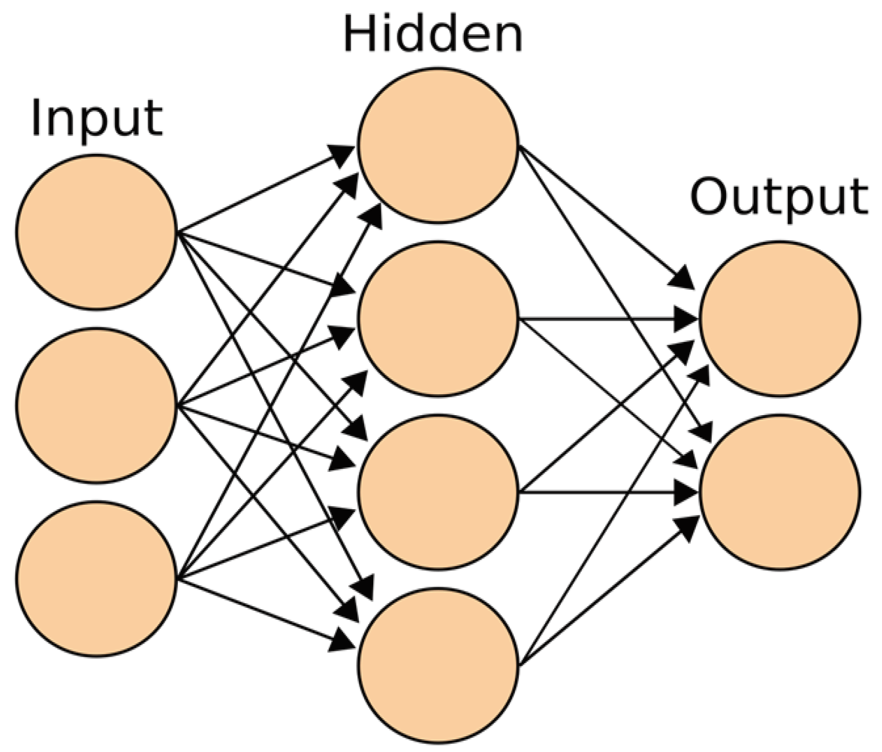
The image illustrates the input, hidden, and output layers. The input layer receives data (e.g., images or text), the hidden layers process the data through various transformations, and the output layer generates results, such as image classification or value prediction.
The learning process of neural networks involves:
- Forward Propagation: Information is passed through the layers.
- Backpropagation: Prediction errors are used to update the weights between neurons.
- Optimization: The goal is to minimize error using algorithms like gradient descent.
Neural networks represent a revolution in data analysis and solving complex problems. The combination of advanced algorithms and innovations, such as nanowire networks, provides opportunities for the development of new applications across various industries. This technology continues to be a key tool in artificial intelligence research and stochastic systems analysis. [2]3
2. Spectrum of Stochastic Methods
Let us assume we have a loss function J() that we aim to minimize to train a model. Stochastic gradient descent (SGD) is used to iteratively update the parameters \theta in the direction of the negative gradient of the loss function. The parameter update can be mathematically expressed as:
θt+1=θt−∇J(θt)
Here, t represents the parameters at the current step, is the learning rate, and ∇J(t) is the gradient of the loss function at t.
The "stochastic" aspect arises when the gradient is approximated using individual samples from the dataset rather than the entire dataset. Instead of using all data points, a single random sample (or a small subset) is used to approximate the gradient. This allows for faster convergence, especially when the dataset is large.
This is one example of stochastic gradient descent, but there exists a broad spectrum of stochastic methods used in optimization and model training [3]. 4Below are some notable methods from this spectrum:
- Stochastic Gradient Descent (SGD):SGD updates model parameters using the negative gradient of the loss function based on individual samples.
- Mini-batch Gradient Descent:This is a variation of SGD where a small subset of data (mini-batch) is used to approximate the gradient instead of single samples. This often leads to more stable convergence compared to pure SGD.
- Adam (Adaptive Moment Estimation):Adam combines the benefits of adaptive learning rates for each parameter and adjusts them over time. It is widely used in optimizing neural networks.
- SGD with Momentum:Adding momentum helps accelerate convergence by utilizing the accumulated gradient from previous steps to "jump over" local minima.
- Monte Carlo Simulations:A general approach for estimating numerical values, often used in statistics and machine learning. Monte Carlo methods employ stochastic sampling to approximate expectations or integral values.
- Stochastic Gradient Descent with Warm Restarts (SGDR):This method uses a cyclical approach to changing the learning rate, helping the model escape local minima and avoid divergence.
- Reparameterization Gradients:Often used in Bayesian learning, this technique employs reparameterization to enable efficient learning of models with stochastic layers.
These are just a few examples. Different methods are optimal in varying scenarios, depending on the characteristics of the data and the optimization problem at hand [4].5
2.1. Stochastic Process
A stochastic process is a mathematical model that describes the evolution of a random variable over time. This process incorporates an element of randomness, meaning that the values of the variable can change according to stochastic or probabilistic rules.
General definitions of a stochastic process include:
- Time Parameter: A stochastic process evolves over time. The time parameter can be discrete (e.g., specific moments in time) or continuous (e.g., continuous time).
- Random Variable: At each moment, the value of the stochastic process is a random variable. This random variable may follow a specific probability distribution.
- Sample Space: A stochastic process can be defined within a sample space that represents all possible values the process can take.
Examples of Stochastic Processes:
- White Noise: A random process with a constant power density across all frequencies. This is a basic example of a stochastic process and is often used in analysis and modeling.
- Archimedean Funnel: A model used to describe the stochastic motion of particles in a fluid.
- Stochastic Differential Processes: Processes frequently used in mathematical finance to model the prices of financial instruments.
Stochastic processes have a wide range of applications in various fields, including statistics, economics, engineering, biology, and other scientific disciplines. By analyzing stochastic processes, researchers can better understand and model natural and social phenomena that are subject to randomness [5].6
ExampleSuppose we have a model that predicts the probability of developing a particular disease () based on several clinical parameters (X). Our goal is to determine the posterior distribution of the parameter using Markov Chain Monte Carlo (MCMC).
Data and Model:
- Dataset (D):We have a dataset D containing information about patients diagnosed with the disease.
- Model:A simple logistic regression model is used to link the parameter \theta with the clinical parameters X.
The logistic regression model predicts the probability of a patient developing the disease based on their clinical parameters, expressed as:
P(∣D)=
Prior Distribution
- We set a prior distribution P() based on assumptions about the expected behavior of the parameter . For example, a uniform distribution can be used if no prior knowledge is available.
Likelihood of Data
- The likelihood P(D∣) is defined as the probability of observing the data D, given the assumed values of the parameter .
Generating MCMC Samples
- We use an MCMC algorithm, such as Metropolis-Hastings or Gibbs sampling, to generate a sequence of samples for the parameter based on the posterior distribution.
Result Analysis
- At the end of the MCMC iterations, we have a sequence of samples for the parameter \theta.
- These samples can be used to compute point estimates of as well as confidence intervals, providing insights into the uncertainty of our estimates.
For example, by analyzing the obtained samples, we may conclude that there is a 95% probability that the true value of the parameter lies within a specific interval. This approach not only provides a point estimate but also valuable information about the uncertainty in the estimate [6].7
2.2. General Mathematical Model
The linear model we aim to estimate is expressed as:
Y=θ·X + ε
Where:
- Y represents the dependent variable (in this case, the values we want to predict).
- X is the independent variable (in this case, the values used for prediction).
- θ is the parameter representing the slope of the linear relationship.
- ε represents the error or noise, included because real-world data is often not perfectly linear [20].8
Using the Bayesian approach, we expressed our prior belief about the parameter using a normal distribution with a mean of =0 and a standard deviation of =1 [19].9
The likelihood of the model describes how the data (variable Y) depends on the parameter and the independent variable X. In our case, it follows a normal distribution around the value X·X, with a standard deviation of =0.1, to account for the noise [17].10
Thus, the combination of the prior distribution and the likelihood model allows us to generate the posterior distribution for using MCMC sampling. Visualizing the trace of the samples enables us to assess how the values of behave during sampling. If convergence is achieved, we expect the traces to stabilize, providing a reliable estimate of the parameter [16].11
import pymc3 as pm
import numpy as np
import matplotlib.pyplot as plt
# Simulate data
np.random.seed()
X = np.linspace(0, 1, 100)
true_slope = 2
noise = np.random.normal(scale=0.1, size=100)
Y = true_slope * X + noise
# Define the model
with pm.Model() as linear_model:
# Prior for slope (theta)
theta = pm.Normal(’theta’, mu=0, sd=1)
# Linear model
Y_pred = pm.Normal(’Y_pred’, mu=theta * X, sd=0.1, observed=Y)
# MCMC sampling
trace = pm.sample(2000, tune=1000)
# Visualize the results
pm.traceplot(trace)
plt.show()
Figure 2.
Histogram of Solution Distribution.
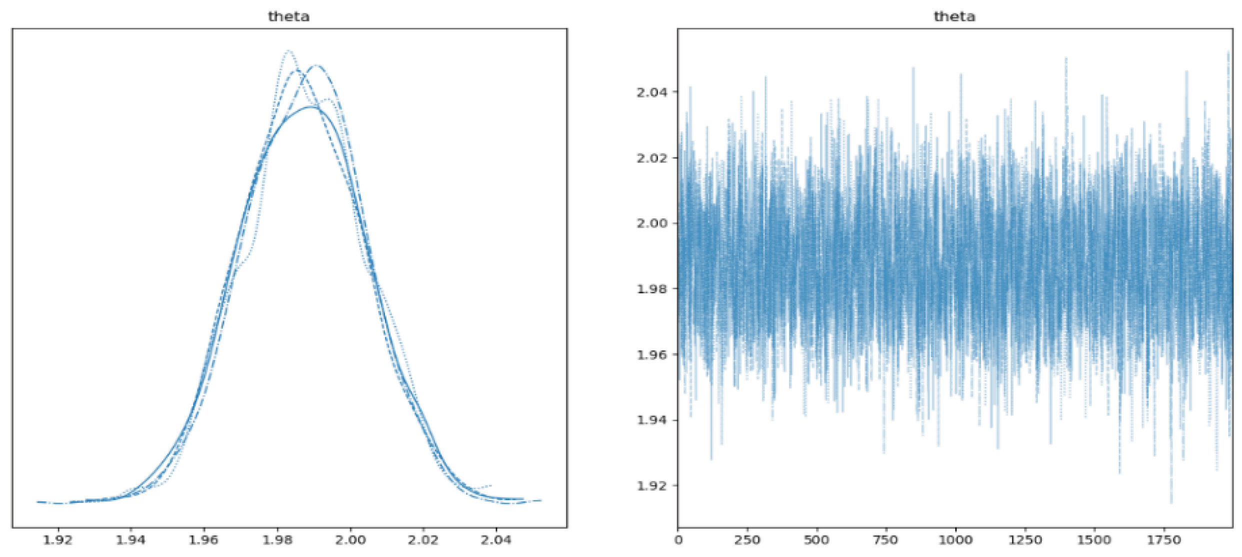
- Left Side: On the left side of the image, you can see a histogram of the values of . This histogram represents the posterior distribution of the parameter after considering the prior distribution and the data. The height of the bars in the histogram indicates the relative probability of specific values. Higher density implies a greater likelihood for that value of the parameter [15].12
- Right Side: On the right side of the image, the trace of values during sampling is displayed. Each line represents the trajectory of throughout the sampling process. This provides a visual check for MCMC convergence. If all traces are stable and aligned, it indicates convergence [7].13
In our specific case, if convergence is achieved, the histogram on the left side is expected to peak around the true value of , while the traces on the right side will be stable and consistent. This visualization allows you to assess the central value and uncertainty of after data analysis using the Bayesian approach.
2.3. Optimization
The model can be used to optimize parameters in the objective function. The objective function is given as:
Where:
- N represents the number of data points,
- Yi represents the actual value at point iii,
- Y∧i represents the predicted value at point iii based on the parameters .
This objective function measures the squared difference between actual and predicted values. Optimizing this function seeks the parameter values that minimize this difference. In our model, represents the slope and intercept parameters of the linear model [14].14
Figure 3.
Optimization of Result Visualization
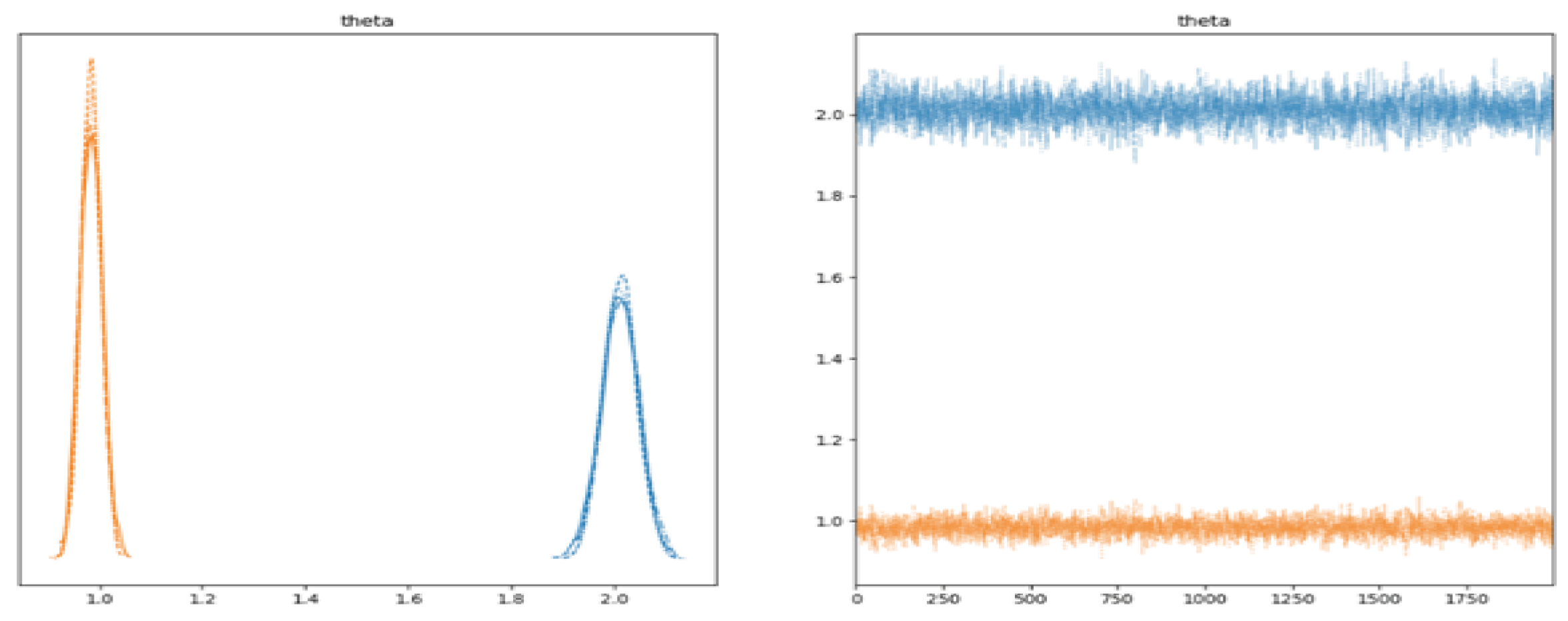
The image displays the results of MCMC sampling for the slope (0) and intercept (1) parameters in a linear model.
- Left Side:The left side shows histograms of the parameter values, illustrating how the samples from the MCMC process are distributed. The height of the bars represents the relative probability of the parameter values [8].
- Right Side:The traces show the paths taken by the parameter values during sampling. If the sampling has converged, the traces are expected to be stable and consistent.
The Maximum A Posteriori (MAP) estimate provides point estimates of the most likely parameter values. In this case, these are the 0 and 1\ values that maximize the posterior distribution [13].15
Finally, the results of the objective function optimization show the parameter values that minimize the squared difference between actual and predicted values. Both approaches (MCMC and optimization) provide parameter estimates while accounting for the uncertainty in the parameters [12].16
This output represents the results of MCMC sampling (Maximum A Posteriori - MAP) and the optimization of the objective function. Here’s what the obtained results signify:
MAP Estimate for Theta
The values of that maximize the posterior distribution of the parameters are:
- Slope (0): 2.012
- Intercept (1): 0.984
These are the point estimates of the most likely parameter values based on the Bayesian analysis of the data [11].17
Objective Function Optimization Using MCMC Samples
The parameter values that minimize the objective function, derived through optimization using MCMC samples, are:
- Slope (0): 2.014
- Intercept (1): 0.983
This optimization accounts for the uncertainty in the parameters by considering the full distribution of parameter values from the MCMC samples.
Summary
The obtained results provide parameter estimates for the linear model while incorporating the uncertainty in these estimates. Both approaches (MAP and optimization) suggest similar parameter values, indicating consistency between the Bayesian approach and classical optimization [9].
2.4. Deep Learning
To apply deep learning in this example, we will use the TensorFlow and Keras libraries. We assume a simple neural network model with one hidden layer.
Figure 4.
Deep Learning Results.
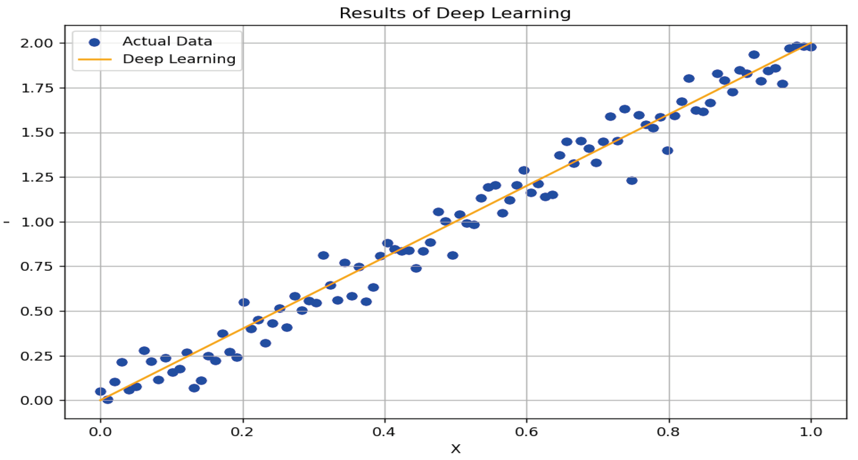
The figure shows the results of deep learning based on a neural network trained on simulated data. Here’s what the figure conveys:
-
Actual Data:
- 1.
- The points on the graph represent actual data generated according to a linear model with added noise. These points form the basis for training the model and demonstrate how the real data is distributed.
-
Deep Learning Results:
- 1.
- The orange line represents the predicted values from the deep learning model based on the trained network. The model attempts to learn the linear dependency between the input X and output Y, while also adapting to the noise in the data.
-
Optimized Parameters:
- 1.
- Below the graph, the optimized parameters of the neural network are displayed. These parameters include the weights and biases used by the model to generate predictions.
This figure enables a visual assessment of how well the model reproduces actual data and how the optimized parameters adjusted during training. High alignment between predicted and actual values indicates the model’s efficiency in approximating the linear dependency in the data.
After training, the optimized parameters of the neural network are as follows:
Optimized theta using Neural Network:
[array([[ 1.3905556 , 1.2045665 , -0.7317417 , 1.011643 , -0.3996426 , 0.15751715, -0.4820116 , -0.3988453 , 0.09923384, -0.7143219 ]],
dtype=float32)
array([ 0.5152299 , 0.49337307, 0. , 0.0124758 , 0. ,
-0.15774246, 0. , 0. , -0.10050173, 0. ],
dtype=float32)
array([[ 0.6120329 ],
[ 0.65885425],
[-0.43376464],
[ 0.36610386],
[ 0.5354449 ],
[-0.57069385],
[-0.10281849],
[-0.47908455],
[-0.11608436],
[ 0.19966263]], dtype=float32)
array([0.34189823], dtype=float32)]
Interpretation of Parameters
- First Row (Weights of the Hidden Layer):The first array represents the weights of the hidden layer. These coefficients are applied to the inputs to generate the outputs of the hidden layer.
- Second Row (Bias of the Hidden Layer):The second array represents the biases of the hidden layer. Bias is a constant added to each neuron in the hidden layer.
- Third Row (Weights of the Output Layer):The third array represents the weights of the output layer. These weights influence the outputs of the hidden layer to generate the final outputs of the network.
- Fourth Row (Bias of the Output Layer):The last value represents the bias of the output layer, a constant added to the network’s output.
These values result from optimization during network training. They reflect the adjustments the model has learned to best approximate the given dataset. The high correspondence between the predicted and actual values suggests the model’s effectiveness in capturing the linear dependency and accounting for noise in the data.
2.5. Application for Solving SPDE
We developed a MATLAB application that enables the simulation of stochastic partial differential equations (SPDE) using three numerical methods: Euler-Maruyama, Milstein, and Runge-Kutta. This application features an intuitive graphical user interface (GUI), allowing users to input initial parameters, select simulation methods, and define new equations through simple steps [10].18
The image shows the application’s layout, where users can input the initial state (x0x_0x0), total simulation time (T), and the number of steps (N). Additionally, users can choose the numerical simulation method by selecting options provided as checkboxes. The buttons "Input New SPDE" and "Run Simulation" enable defining new equation functions and starting the simulation.
An additional window, accessible by clicking on "Input New SPDE," allows users to specify mathematical functions for the deterministic part (a(x,t)), the noise coefficient (b(x,t)), and the delay function (p(t)). After defining the new functions, the user can run the simulation and analyze the graphical representation of the solution x(t).
This application is designed for researchers and engineers who want to quickly and easily experiment with SPDE equations and their numerical solutions. Its intuitive design makes it suitable for various applications in science, finance, and engineering.
Figure 5.
Aplication for SDE Simulations methods.
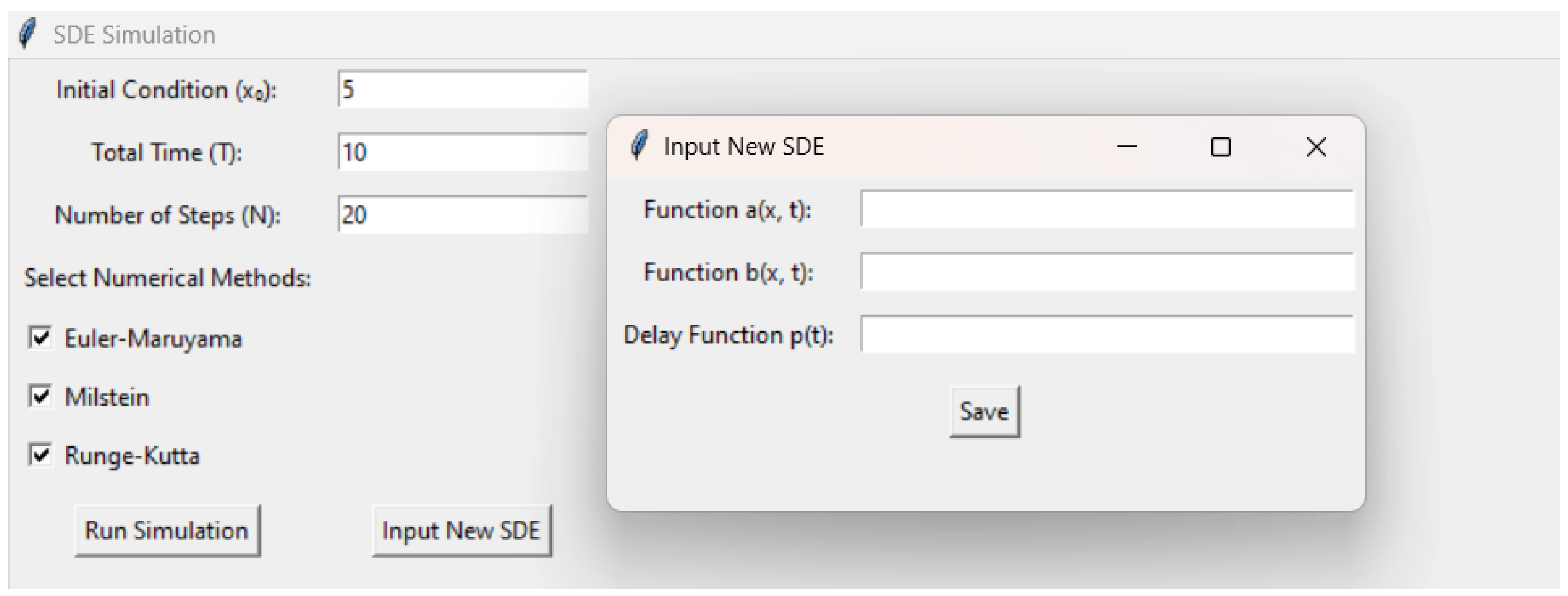
Graphical Interface of the SPDE Solving Application
The application allows users to customize equations by entering new functions. For example, if a user wants to simulate a system with the equation:
they can input the following:
a(x,t)=-x/5
b(x,t)=sin(t)x
p(t)=0.1+0.05cos(t).
After entering these functions through the Input New SPDE option, the application uses the selected numerical method for simulation and generates a graph illustrating the system’s behavior over time.
The visualization of the solution provides users with insights into the dynamics of the modeled process, including the effects of stochastic noise and deterministic components. This makes the application adaptable for various scientific and engineering applications, from modeling physical systems to financial analyses.The image illustrates the graphical interface of the SPDE application. Users can:
- Enter initial parameters such as initial condition (x0x_0x0), total simulation time (T), and the number of steps (N).
- Select numerical methods like Euler-Maruyama, Milstein, or Runge-Kutta.
- Use the Input New SPDE option to define new functions for a(x,t), b(x,t), and p(t).
- Visualize the simulation results as a graph, which shows how the system evolves over time.
The graphical interface is intuitive and provides tools for easy configuration and simulation, enabling users to experiment with different equations and analyze the results efficiently.In conclusion, the application offers flexibility in defining equations and selecting simulation methods, facilitating the exploration and analysis of complex systems. This flexibility makes it suitable for a wide range of users, from students to researchers and professionals.
3. Conclusion
In this study, we explored various numerical algorithms for solving stochastic partial differential equations (SPDE), including the Euler-Maruyama, Milstein, and Runge-Kutta methods. Beyond traditional methods, we implemented a neural network-based approach, enabling the prediction of complex system behaviors through hyperparameter optimization and network training analysis.
The simulation results revealed significant differences in accuracy among the methods, with the Runge-Kutta method serving as a reference solution due to its high precision. The Euler-Maruyama method demonstrated speed but was more approximate, while the Milstein method improved accuracy by incorporating additional corrective terms. Error analysis highlighted the strengths and limitations of each method, providing a clear visualization of deviations.
By introducing neural networks into the SPDE-solving process, we took a step toward optimizing solutions for cases where traditional methods are inefficient for high-dimensional or complex nonlinear problems. Deep learning algorithms enabled more precise approximations, though their effectiveness depended on careful tuning of parameters such as the number of layers, neurons, and learning rates.
Optimization was a key aspect of the study for both numerical methods and neural networks:
- For numerical algorithms, optimization focused on selecting the time step (dtdtdt), balancing precision and computational cost. Adaptive time-stepping could further reduce errors.
- For neural networks, the optimization process involved training through epochs, choosing activation functions, and minimizing network error. Various architectures were tested to achieve the best possible accuracy.
Numerical algorithms remain a standard and efficient approach for solving SPDEs, particularly when stability and a well-defined solution structure are essential. On the other hand, neural networks offer significant potential for future research, especially in cases where traditional methods face limitations. Combining these two approaches could create hybrid models that merge the accuracy of numerical methods with the flexibility of neural networks, opening new possibilities for solving complex stochastic problems. Future efforts could include implementing adaptive algorithms, improving regularization in networks, and extending applications to higher-dimensional domains, further enhancing the precision and applicability of these methods. Such advancements could pave the way for more robust solutions to SPDEs and other stochastic challenges.
References
- Bishop, C. M. (2006). Pattern Recognition and Machine Learning. Springer. [CrossRef]
- Bishop, C. M. (2006). Pattern Recognition and Machine Learning. Springer. [CrossRef]
- Čajić, E., & Stojanović, Z. (2023). Stochastic Methods in Artificial Intelligence. Research Square. [CrossRef]
- Čajić, E., Nićin, S., Omerović, M., & Shabani, E. (2023). Stochastic Optimization of Surface Roughness Using Monte Carlo Algorithms. ResearchGate. Available online: https://www.researchgate.net/publication/380828878_Stochastic_Optimization_of_Surface_Roughness_Using_Monte_Carlo_Algorithms.
- Dedić, V., & Stanković, R. S. (2012). Fourier Analysis on Finite Non-Abelian Groups with Applications in Signal Processing. Springer. [CrossRef]
- Getoor, L., & Taskar, B. (Eds.). (2007). Introduction to Statistical Relational Learning. MIT Press. [CrossRef]
- Goodfellow, I., Bengio, Y., & Courville, A. (2016). Deep Learning. MIT Press. Available online: https://www.deeplearningbook.org.
- Higham, N. J. (2002). Accuracy and Stability of Numerical Algorithms (2nd ed.). Society for Industrial and Applied Mathematics. [CrossRef]
- Karniadakis, G. E., Kevrekidis, I. G., Lu, L., Perdikaris, P., Wang, S., & Yang, L. (2021). Physics-informed machine learning. Nature Reviews Physics, 3(), 422–440. [CrossRef]
- Kloeden, P. E., & Platen, E. (1992). Numerical Solution of Stochastic Differential Equations. Springer. [CrossRef]
- Koller, D., & Friedman, N. (2009). Probabilistic Graphical Models: Principles and Techniques. MIT Press. [CrossRef]
- LeCun, Y., Bengio, Y., & Hinton, G. (2015). Deep learning. Nature, 521(7553), 436–444. [CrossRef]
- Milstein, G. N. (1995). Numerical Integration of Stochastic Differential Equations. Springer. [CrossRef]
- Murphy, K. P. (2012). Machine Learning: A Probabilistic Perspective. MIT Press. [CrossRef]
- Raissi, M., Perdikaris, P., & Karniadakis, G. E. (2019). Physics-informed neural networks: A deep learning framework for solving forward and inverse problems involving nonlinear partial differential equations. Journal of Computational Physics, 378, 686–707. [CrossRef]
- Särkkä, S., & Solin, A. (2019). Applied Stochastic Differential Equations. Cambridge University Press. [CrossRef]
- Schmidhuber, J. (2015). Deep learning in neural networks: An overview. Neural Networks, 61, 85–117. [CrossRef]
- Sarker, I. H. (2022). AI-Based Modeling: Techniques, Applications and Research Issues Towards Automation, Intelligent and Smart Systems. SN Computer Science, 3(), 158. [CrossRef]
- Sutton, R. S., & Barto, A. G. (2018). Reinforcement Learning: An Introduction (2nd ed.). MIT Press. Available online: https://www.andrew.cmu.edu/course/10-703/textbook/BartoSutton.pdf.
- Zhang, H., & Chen, Y. (2021). Stochastic Processes and Their Applications in Artificial Intelligence. In Stochastic Processes and Their Applications in Artificial Intelligence (pp. 1–20). IGI Global. [CrossRef]
| 1 | |
| 3 | |
| 4 | |
| 5 | |
| 6 | |
| 7 | |
| 8 | |
| 9 | |
| 10 | |
| 11 | |
| 12 | |
| 13 | |
| 14 | |
| 15 | |
| 16 | |
| 17 | |
| 18 |
Disclaimer/Publisher’s Note: The statements, opinions and data contained in all publications are solely those of the individual author(s) and contributor(s) and not of MDPI and/or the editor(s). MDPI and/or the editor(s) disclaim responsibility for any injury to people or property resulting from any ideas, methods, instructions or products referred to in the content. |
© 2025 by the authors. Licensee MDPI, Basel, Switzerland. This article is an open access article distributed under the terms and conditions of the Creative Commons Attribution (CC BY) license (http://creativecommons.org/licenses/by/4.0/).
Copyright: This open access article is published under a Creative Commons CC BY 4.0 license, which permit the free download, distribution, and reuse, provided that the author and preprint are cited in any reuse.


