
Submitted:
22 January 2025
Posted:
22 January 2025
You are already at the latest version
Abstract
Traditional methods of electroencephalograms(EEG) data augmentation, such as segmentation-reassembly and noise mixing, suffer from data distortion that can alter the original temporal and spatial feature distributions of the brain signals. Deep learning-based methods for generating augmentation EEG data, such as Generative Adversarial Networks (GANs) and Variational Autoencoders (VAEs), have shown promising performance but require a large number of comparative learning samples for model training. To address these issues, this paper introduces an EEG data augmentation method based on Gaussian Mixture Model microstates, which retains the spatiotemporal dynamic features of the EEG signals in the generated data. The method first performs Gaussian mixture clustering on data samples of the same class, using the product of the probability coefficients and weight matrices of each Gaussian model as corresponding microstate features. Next, it randomly selects two EEG data samples of the same type, analyzes the similarity of the main components of the microstate features, and swaps the similar main components to form new Gaussian mixture model features. Finally, new data is generated according to the Gaussian mixture model using the respective model probabilities, weights, means, and variances. Experimental results on publicly available datasets demonstrate that the proposed method effectively characterizes the original data's spatiotemporal and microstate features, improving the accuracy of subject task classification.
Keywords:
EEG
; Gaussian mixture model
; microstate
; feature
; data augmentation
1. Introduction
Electroencephalograms (EEG) are biological signals generated by brain neural activity, reflecting the physiological state of the brain. EEGs record the spontaneous and rhythmic electrical activity of groups of brain cells through electrodes. Due to their safety, portability, ease of use, high temporal resolution, and low cost, EEGs are widely used in medical and cognitive neuroscience research fields [1].
However, commonly used scalp EEG signals exhibit characteristics such as nonlinearity, non-stationarity, broad frequency bands, and a low signal-to-noise ratio (SNR) [2]. These traits pose significant challenges for research and application. Firstly, the potential signals from within the skull are conducted through layers of tissues, fluids, bones, etc., to reach the scalp, where they are easily interfered with by physiological and non-physiological signals, reducing SNR [3]. Secondly, due to the high level of attention required during data collection, it is difficult to obtain large amounts of brain data, leading to small sample characteristics [4]. Thirdly, the signal data changes over time and is non-stationary and nonlinear [5,6], resulting in poor generalization performance of computational models for EEG processing. Fourthly, there are significant individual differences in EEG signals, further limiting the generalization performance of EEG processing models.EEG models trained on specific individuals may perform poorly on new individuals [7,8]. Additionally, a large amount of redundant information or non-specific information unrelated to the target interferes with the key physiological information in the EEG signals. Therefore, it is necessary to increase samples, denoise, and transform EEG data to generate new datasets with better diversity and robustness, thereby improving model generalization, reducing overfitting, and enhancing model analysis accuracy.
Traditional EEG data augmentation methods mainly include the following:
Firstly, methods based on data morphology changes [9,10]. These methods simulate the effects of factors such as head movement and muscle tension on EEG data, generating data with better representation of temporal and frequency variations based on the original EEG data . However, these geometrically transformed data may destroy the time domain and frequency features [11,12].
Secondly, methods based on signal segmentation and recombination [13,14,15,16]. This method segments specific time window EEG data according to the temporal characteristics of the EEG signal and reconstructs new data by randomly selecting fragments. Assuming is an EEG signal set with a specific category, (i=1…N, = N indicates the total number of samples), where N represents the number of sampling points in each sample. Each EEG waveform is divided into k non-overlapping consecutive segments, forming a dataset containing data fragments. New EEG samples are then generated by randomly concatenating K segments from , repeating the operation until the desired number of signals is obtained.These methods are intuitive and simple but may exacerbate model overfitting due to the similarity after augmentation [17,18,19,20]. Another common method is adding noise. This method adds random matrices from Gaussian distributions (Gaussian or salt-and-pepper noise) to the original EEG data to simulate real-world noise interference for data augmentation. This method can effectively increase dataset diversity and improve model robustness [21,22,23]. However, introducing artifacts in the original signal makes it difficult to verify the true psychological state response of the new EEG signal, complicating model accuracy validation.
Thirdly, methods based on data transfer. This method transfers existing same-type EEG data to new environments to improve model performance. It usually uses auxiliary data from the source domain to support training in similar domains. This method may lead to data distortion and affect model accuracy [24].
Fourthly, methods based on data generation. There are two main types here: Variational Autoencoders (VAE), consisting of an encoder and a decoder, where the encoder converts original data into latent data, and the decoder maps latent data back to real data. To generate new data, VAE randomly samples points from the learned latent space and passes these samples through the decoder network to reconstruct them as new samples. The drawback of this method is the need for a large number of data samples [25,26]. Generative Adversarial Networks (GAN) and their variants can generate synthetic data through training generative and discriminative networks [27,28,29]. The generative network accepts random noise from a specific distribution (e.g., Gaussian) and attempts to generate realistic-like synthetic data, while the discriminative network is trained to classify between real and synthetic data. These two networks are adversarial; after sufficient training, the generative network produces similar signals. [30,31,32] The common drawback of these methods is that they require a certain amount of data to support the adversarial training of generators and discriminators, which conflicts with the goal of data augmentation on small training sets, and also consumes substantial computational resources and presents replication difficulties [33,34,35].
Existing methods for increasing EEG data samples either require a large number of comparison learning samples or generate new data that alters the original EEG’s spatiotemporal features, leading to data distortion. Researching a new data augmentation method that does not require extensive original data samples while preserving the spatiotemporal dynamic features of similar EEG signals is significant for improving EEG processing algorithms.
Microstate analysis is one of the EEG signal analysis methods, capable of characterizing quasi-steady-state scalp potential fields on a sub-second scale and retaining the temporal dynamics and spatial information of scalp potential distributions, representing a novel form of EEG signal quantification with potential neurophysiological relevance [36,37]. Our paper reconstructs new EEG data based on Gaussian microstate features. Firstly, Gaussian Mixture Models (GMM) decompose same-type sample EEG signals to obtain microstate feature parameters for each sample, using the probability of Gaussian submodels. Secondly, random selection of two same-type samples analyzes the similarity of principal components, and exchanges and reassembles principal components with similar features to form new submodel probabilities. Finally, new data is generated based on submodel probabilities, weight values, means, and variances.
(1) Proposing an EEG data augmentation method based on GMM microstate feature reconstruction. Firstly, GMM clustering is performed on same-type data samples to obtain microstate features of each sample type, using Gaussian submodel probabilities. Secondly, random selection of two same-type samples analyzes the similarity of principal components and exchanges principal components with similar features to form new submodel probabilities. Finally, new data is generated based on submodel probabilities, weights, means, and variances.
(2) By analyzing the newly added EEG samples and original EEG samples from traditional EEG data augmentation methods in terms of time and space features, we demonstrate the differences in spatiotemporal features among the methods.
(3) Classification tasks are performed on EEG generated by traditional methods and the method proposed in this paper to compare improvements in classification performance.
The rest of this paper is organized as follows. Section 2 mainly introduces our proposed method and experimental data, including the implementation of Gaussian microstate feature reconstruction. Section 3 primarily discusses experiments and results. Section 4 discusses and analyzes experimental results. Finally, Section 5 summarizes this work.
2. Materials and Methods
2.1. The BCI Competition IV Dataset 2a
The publicly available dataset BCI Competition IV 2a is an electroencephalogram (EEG) dataset based on visually induced motor imagery, collected by the American Enco company [38]. The experiment was conducted with 9 participants, each completing two sessions. Each session included data from 4 categories, with 7 trials per category. Therefore, each participant contributed a total of 288 trials, comprising 72 trials for left-hand motor imagery, 72 trials for right-hand motor imagery, 72 trials for feet motor imagery, and 72 trials for tongue motor imagery.
Data preprocessing: The EEG dataset is pre-processed using Python 3.8.8 and the MNE 0.23.4 toolkit.Baseline Correction, Principal Component Analysis (PCA), and Artifact Rejection preprocessing steps are detailed in the article [39] published by Liao et al.
2.2. EEG Microstates and Gaussian Microstate
2.2.1. EEG Microstates
Originating from Lehmann et al. in 1987, multi-channel EEG recordings can be composed of a series of quasi-stable microstates, each characterized by the topological structure of the entire channel terrain map [36,37]. This representation is an effective method that helps us understand the dynamic processes of the brain during information processing, as well as functional changes under different tasks and states. It holds significant importance for fields such as cognitive neuroscience, clinical diagnosis, and rehabilitation therapy. As shown in Figure 1, EEG microstate analysis includes the following steps:
Microstate Feature Extraction: Key features such as duration, frequency of occurrence, and spatial distribution are extracted from each microstate. These features can reflect functional changes in the brain under different tasks and states.
Microstate Detection: EEG signals are divided into different microstates through specific algorithms (such as clustering analysis). Each microstate represents a transient functional state of the brain, usually lasting from tens to hundreds of milliseconds.
Statistical Analysis: Extracted microstate features are statistically analyzed to reveal patterns and differences in brain activity under different conditions. For example, comparing microstate features under different cognitive tasks or pathological states can help study abnormalities and plasticity of brain function.
Result Interpretation: Based on the results of statistical analysis, combined with knowledge from neuroscience and psychology, changes in brain activity are interpreted and inferred. This aids in our better understanding of the brain’s functions and structure, as well as its role in cognitive and behavioral processes.
2.2.2. Gaussian Microstate
Gaussian Mixture Model-Based EEG Microstates, a distinction from Traditional EEG Microstates Unlike traditional EEG microstates, Gaussian Mixture Model (GMM)-based EEG microstates are distinguished by their use of GMM to decompose EEG microstates into a mixture representation rather than a unique one-hot representation. It has been proven that the classification capability of the GMM-based microstate model under MI tasks is Augmentation [39].
As shown in Table 1, taking a ten-component Gaussian Mixture Model (GMM) as an example, the preprocessed electroencephalogram (EEG) data serves as the input to the model and is a three-dimensional dataset. Here, N represents the number of sensors on the EEG device, corresponding to the variable ’channel’ in the table; T is the number of sampling points per sample, corresponding to the variable ’n_samples’ in the table. The variable ’n_components’ indicates the number of submodels in the GMM, which is set to 10.
Ultimately, the multi-channel EEG data is decomposed into a linear combination of multiple Gaussian submodels. Similar to the one-hot representation model for MI EEG, the GMM mixture representation model extracts dynamic statistical features based on the probability of each submodel. These features include three characteristics as shown in Figure 2: duration, frequency of occurrence, and coverage.
2.3. Gaussian Mixture Model-Based EEG Data Augmentation Method
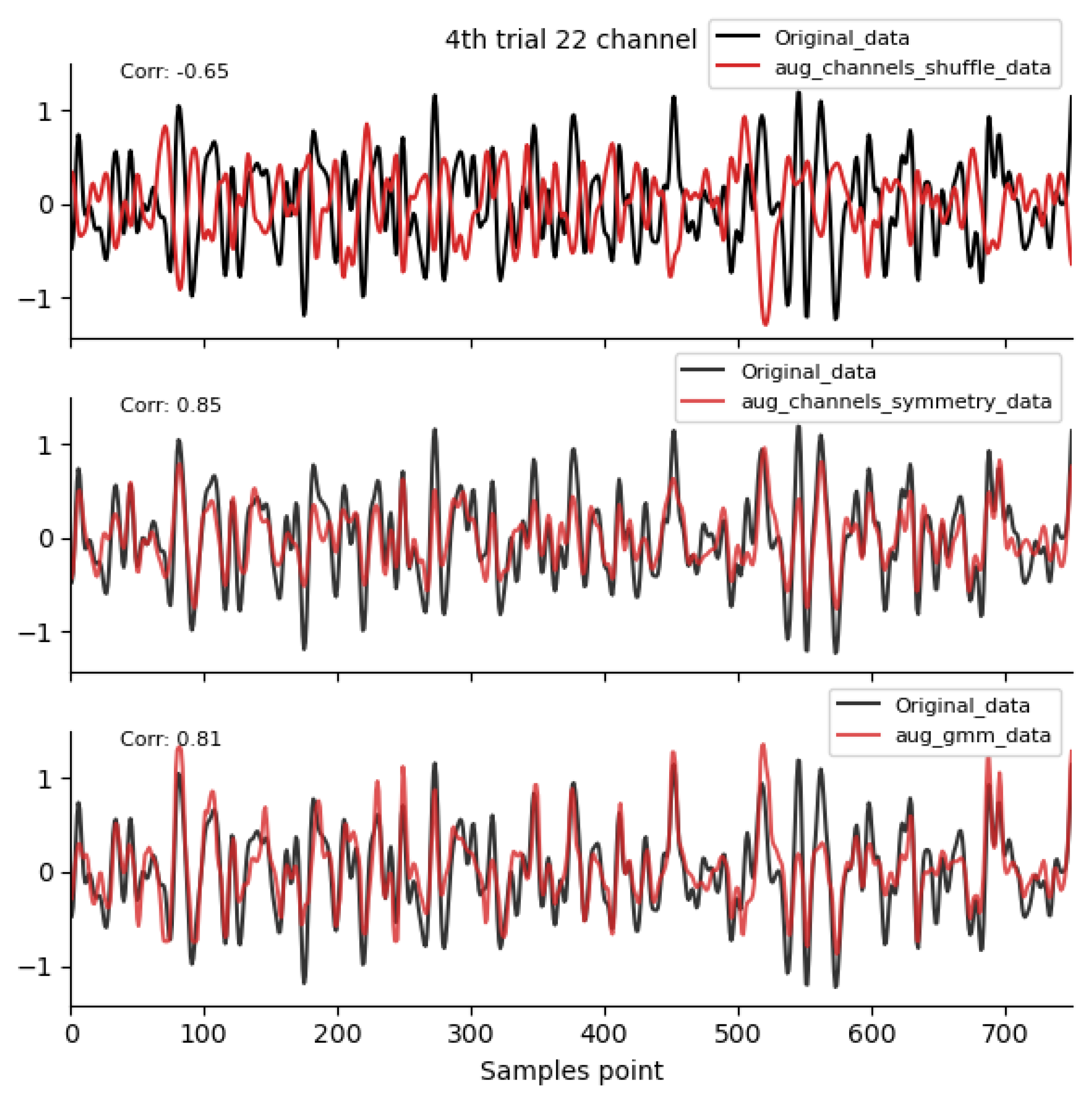
This paper decomposes EEG microstates into a mixture representation, meaning that each sampling point of the multi-channel raw EEG data sample can be decomposed into a linear combination of multiple Gaussian distributions. The duration and frequency or coverage of each Gaussian submodel at each sampling point form the microstate features, encompassing spatiotemporal dynamic information. Then, points with the same feature across different samples are randomly exchanged while maintaining the overall characteristics of the samples. This is followed by inverse reconstruction to synthesize new EEG data. The overall principle is shown in Figure 3, and the algorithm is presented in Table 1. This method increases data diversity and complexity by combining the original EEG signals with noise or distortion signals generated by GMM (Gaussian Mixture Model). As illustrated by the aug_gmm waveform curve in Figure 6 and the brain topographic maps in Figure 10, the signal exhibits more uncertain variations. This approach helps the model learn more robust feature representations, enhancing its ability to recognize different physiological states or cognitive processes.
2.3.1. Gaussian Microstate Decomposition
As shown in Figure 3a, during the decomposition process, we first preprocess the original EEG data, then apply Gaussian Mixture Model clustering to calculate the product matrix of weights and probabilities for adjacent data points with the same label. Points with a similarity coefficient greater than a threshold are exchanged to obtain a new microstate feature matrix. The steps are as follows:
Step 1: Preprocess the original data with filtering, denoising, and other operations.
Step 2: Conduct Gaussian clustering on the data based on labels to obtain the probability, weight, mean, and variance for each category.
Step 3: Multiply the weight of each sample by the probability matrix to obtain the microstate feature matrix.
Step 4: Calculate the similarity coefficients of the microstate feature matrix points for adjacent data with the same label. For points with a similarity coefficient greater than 0.8, exchange their positions to generate a new microstate feature matrix. The purpose is to reduce overfitting in the generated data.
2.3.2. Gaussian Microstate Reconstruction
As shown in Figure 3b, during the reconstruction process, we set a random seed to ensure the reproducibility of the results. For each sample, a channel is randomly selected, and the original data and fitted data are exchanged for that channel, ultimately generating new EEG data. The steps are as follows:
Step 1: Combine the microstate feature matrix with the mean and variance to refit the EEG data.
Step 2: Set a random seed to ensure the reproducibility of the results.
Step 3: Randomly select a channel for each sample according to a certain probability.
Step 4: Exchange the original data and fitted data for the corresponding channel.
Step 5: Reconstruct to obtain new EEG data.
2.4. Other Augmentation Methods
To evaluate the effectiveness of the EEG data augmentation method proposed in this paper, we employed nine different data augmentation techniques. These techniques cover time domain, frequency domain, spatial domain, or other comprehensive transformations.
Figure 4.
Time-domain augmentation method waveform diagram.Data source: Subject 1, Trial 4, Left-hand Motor Imagery, Channel 22.
Figure 4.
Time-domain augmentation method waveform diagram.Data source: Subject 1, Trial 4, Left-hand Motor Imagery, Channel 22.
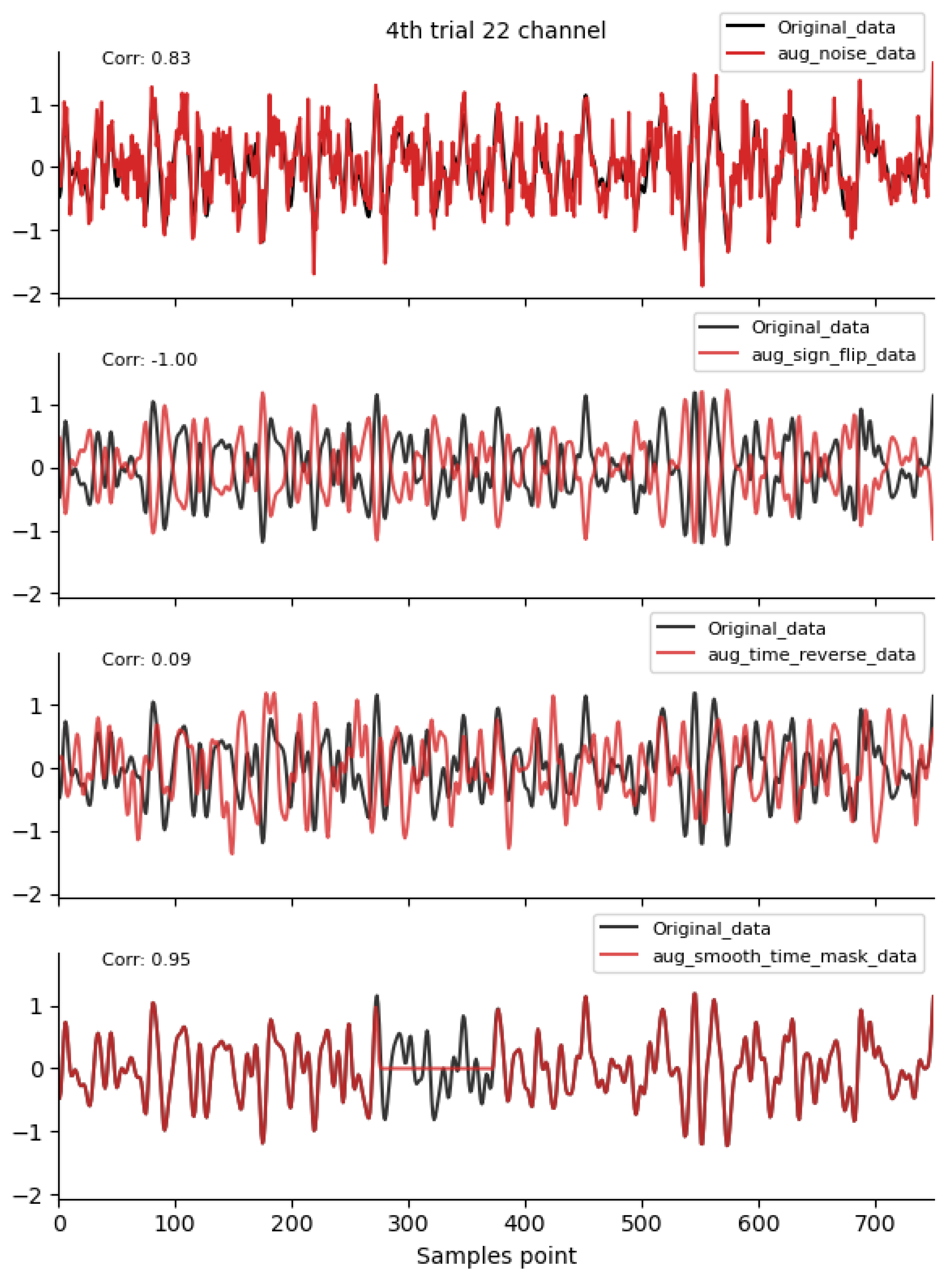
Figure 5.
Frequency-Domain augmentation method waveform diagram.Data source: Subject 1, Trial 4, Left-hand Motor Imagery, Channel 22.
Figure 5.
Frequency-Domain augmentation method waveform diagram.Data source: Subject 1, Trial 4, Left-hand Motor Imagery, Channel 22.
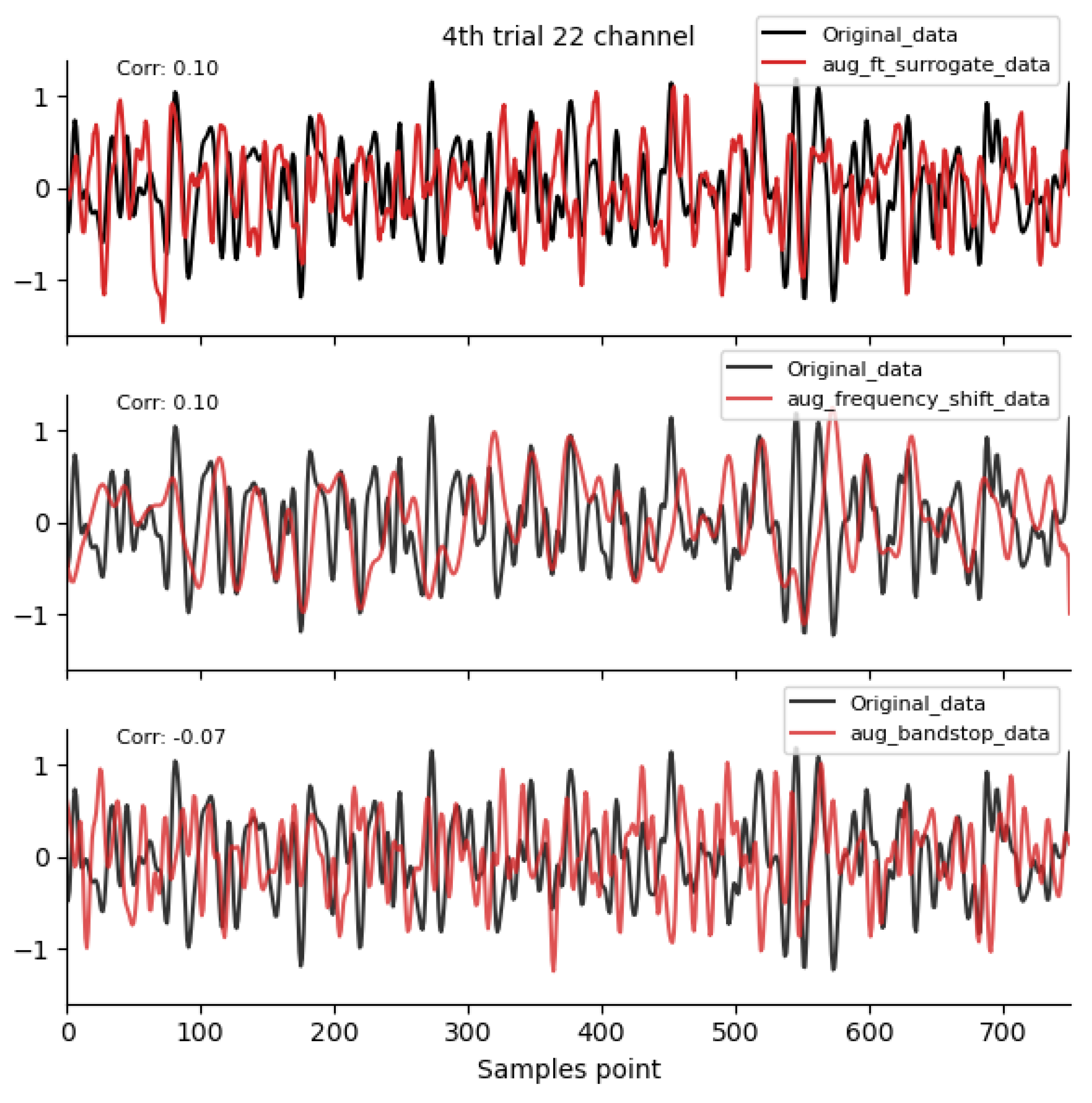
Figure 6.
Spatial-Domain and GMM augmentation methods waveform diagram.Data source: Subject 1, Trial 4, Left-hand Motor Imagery, Channel 22.
Figure 6.
Spatial-Domain and GMM augmentation methods waveform diagram.Data source: Subject 1, Trial 4, Left-hand Motor Imagery, Channel 22.
2.4.1. Time-Domain Augmentation Methods
Noise Addition: By superimposing noise signals onto the original signal, we simulate interference and distortion in real-world environments [22,23]. This accounts for variations in different environments, device differences, or signal transmission disturbances. As shown by the aug_noise curve in Figure 4, the waveform changes after adding noise. The brain topographic maps in Figure 7 reflect how the intensity and distribution of signals in different regions are affected by noise to varying degrees, thereby increasing data complexity and diversity. This helps the model learn more robust feature representations, enhancing its ability to recognize different physiological states or cognitive processes.
Assuming the original signal is , where t represents time, and represents noise, which could be Gaussian white noise, uniform white noise, salt-and-pepper noise, etc. The augmented signal can be expressed as:
Time Reverse: By reversing the signal in time, we increase data diversity [23]. This is demonstrated by the aug_time _reverse curve in Figure 4. The mathematical representation is relatively straightforward, primarily involving reversing the time sequence of the signal.
Assuming the original signal is , where t represents time, the time-reversed signal can be expressed as:
Time Masking: By randomly selecting a continuous segment on the time axis and setting its values to zero, we simulate noise or distortion [23].As shown by the aug_smooth _time_mask curve in Figure 4, the signal is completely set to zero within a certain time interval. This treatment may appear as a sudden drop or disappearance of signal intensity in specific regions during the corresponding time intervals in the brain topographic maps in Figure 5, thereby simulating signal interference or loss scenarios.
Assuming the original signal is , where t represents time, the mathematical representation of the symmetric transformation is:
where is the masking function, taking values of 0 or 1.
Sign Flip: By flipping the sign of the signal, we convert positive signals to negative and vice versa [23]. As shown by the aug_sign_flip curve in Figure 4, the waveform undergoes a reversal between positive and negative values. In the brain topographic maps in Figure 7, this change manifests as an opposite distribution of positive and negative signals in certain regions compared to the original signal, increasing data diversity.
Assuming the original signal is , where t represents time, the mathematical representation of the sign flip transformation is:
2.4.2. Frequency-Domain Augmentation Methods
Frequency Shift: By shifting the frequency of the signal, we alter its frequency components [23]. As shown by the aug_frequency_shift curve in Figure 5, the frequency components of the waveform undergo a shift. In the brain topographic maps in Figure 8, this may reflect changes in the spatial distribution of different frequency components, indicating that the dominant frequencies in certain regions differ from the original signal, thereby simulating different physiological states or cognitive processes.
Assuming the original signal is and is the amount of frequency shift, the mathematical representation of the frequency shift transformation is:
Fourier Transform Surrogate: By computing the Fourier transform of the EEG signal and generating a surrogate signal, we alter the frequency-domain characteristics of the signal [17]. As shown by the aug_ft_surrogate curve in Figure 5, the waveform undergoes changes in its frequency components. In the brain topographic maps in Figure 8, this may reflect variations in the spatial distribution of different frequency components, aiding the model in learning richer frequency-domain information.
Assuming is the original signal and is the frequency-domain signal after the Fourier transform, the mathematical representation of the Fourier transform is:
Bandstop Filter: A signal processing technique used to block signals within a specific frequency range while allowing other frequencies to pass through [23]. It is useful in many applications, such as removing power line noise from electrocardiogram (ECG) signals or eliminating interference in specific frequency bands in electroencephalogram (EEG) signals. This is demonstrated by the aug_bandstop_filter curve in Figure 5. The transfer function of a bandstop filter typically consists of two low-pass filters and one high-pass filter.
Assuming we have a bandstop filter with a center frequency of fc and a bandwidth of B, its transfer function can be expressed as:
where: is the transfer function of the low-pass filter with a cutoff frequency of . is the transfer function of the high-pass filter with a cutoff frequency of .
2.4.3. Spatial-Domain Augmentation Methods
Channel Symmetry: This method involves applying a form of symmetric transformation to signals recorded from different electrodes [19]. As shown by the aug_channels_symmetry curve in Figure 6, this may result in waveforms exhibiting some degree of symmetry between different electrodes. In the brain topographic maps in Figure 9, this change may cause the signal distribution between different regions to exhibit symmetric patterns, aiding the model in learning the interrelationships and independence among various channels.
Assuming the original signal is , where t represents time and i indicates the electrode number, the mathematical representation of the symmetric transformation is:
where n is the total number of electrodes.
Channel Shuffle: By randomly shuffling the order of signals recorded from different electrodes, we alter the correspondence between the electrodes [20]. As shown by the aug_channels_shuffle curve in Figure 6, this results in changes to the correspondence between waveforms across different electrodes. In the brain topographic maps in Figure 9, this change may cause the signal distribution in different regions to become chaotic or disordered, increasing the complexity and diversity of the data.
Assuming the original signal is , where t represents time and i indicates the electrode number, the mathematical representation of the shuffling transformation is:
where is a random permutation function.
3. Experiment and Results
3.1. Comparison of Data Characteristics Generated by Different Augmentation Methods
Figure 4 shows the time-domain waveforms of the first participant, the first trial, imagined left-hand movement, and channel 22 for data generated by ten EEG data augmentation methods. Figure 10 displays the brain topographic maps of the first subject, the fourth trial, imagined left-hand movement, and frequency bands 0–4 Hz (Delta), 4–8 Hz (Theta), 8–13 Hz (Alpha), and 13–30 Hz (Beta) for data generated by the same ten EEG data augmentation methods.
Figure 7.
Time-domain augmentation method for brain topographic maps using left-hand motor imagery.Data source: Subject 1, Trial 4.
Figure 7.
Time-domain augmentation method for brain topographic maps using left-hand motor imagery.Data source: Subject 1, Trial 4.
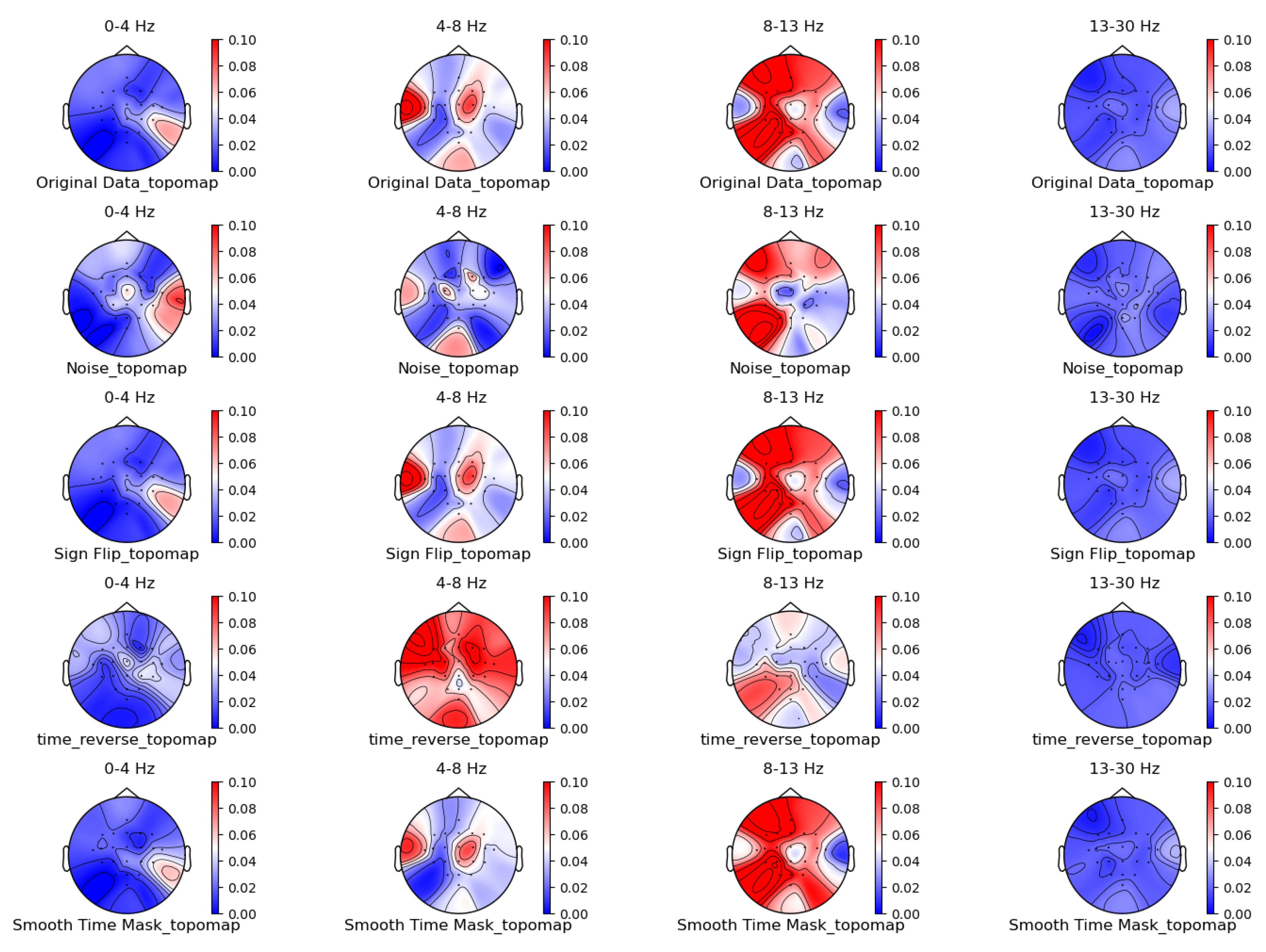
Figure 8.
Frequency-Domain augmentation method for brain topographic maps using left-hand motor imagery.Data source: Subject 1, Trial 4.
Figure 8.
Frequency-Domain augmentation method for brain topographic maps using left-hand motor imagery.Data source: Subject 1, Trial 4.
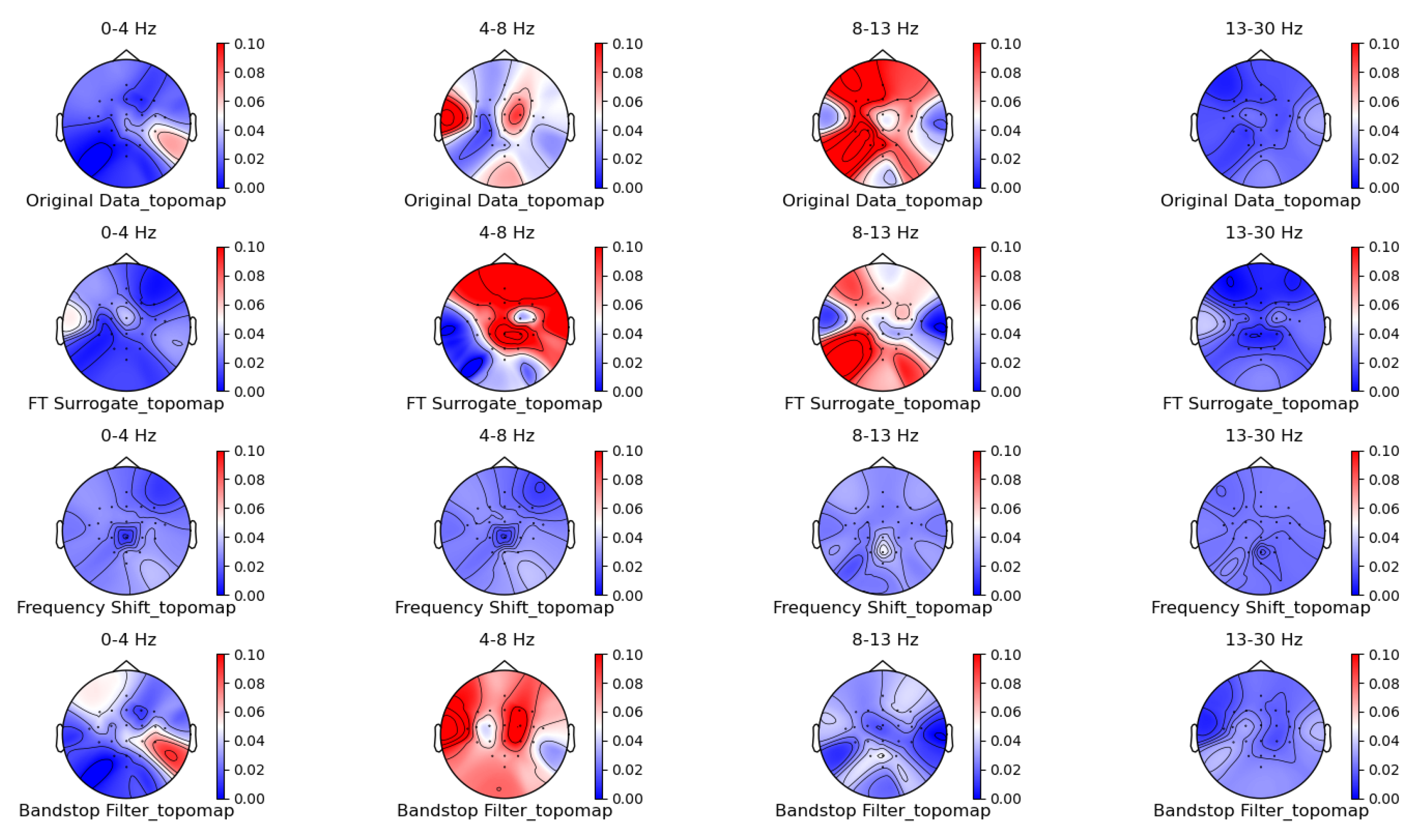
Figure 9.
Spatial-Domain augmentation method for brain topographic maps using left-hand motor imagery.Data source: Subject 1, Trial 4.
Figure 9.
Spatial-Domain augmentation method for brain topographic maps using left-hand motor imagery.Data source: Subject 1, Trial 4.
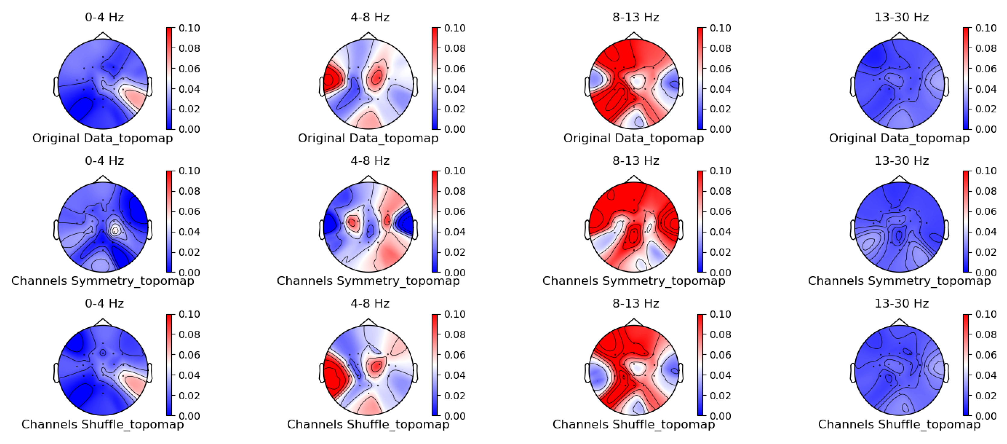
Figure 10.
GMM augmentation method for brain topographic maps using left-hand motor imagery.Data source: Subject 1, Trial 4, Left-hand Motor Imagery.
Figure 10.
GMM augmentation method for brain topographic maps using left-hand motor imagery.Data source: Subject 1, Trial 4, Left-hand Motor Imagery.
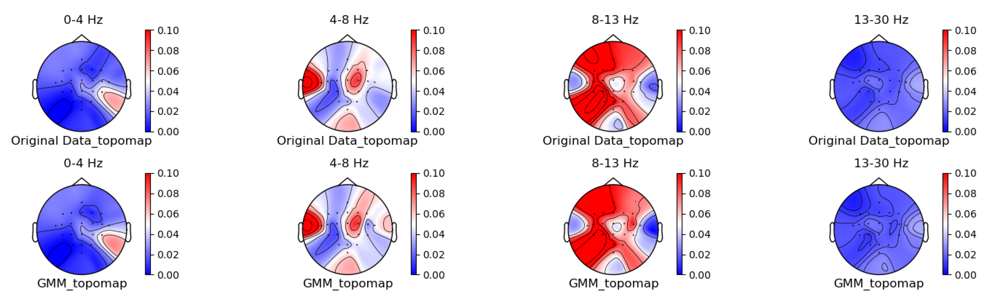
From the original data brain topographic maps, it is evident that different frequency bands exhibit significant variations in activity across various brain regions. Specifically, the wave band (8-13 Hz) shows the most pronounced activity in the frontal and occipital lobes. The activation of these areas is closely related to the planning, simulation, and execution of imagined left-hand movements. In contrast, other frequency bands such as waves, waves, and waves show relatively weaker activity during imagined left-hand movement tasks and have less distinct associations with specific brain regions compared to the wave band.
Looking at the brain topographic maps from each augmentation method, methods such as signal flipping, time masking, channel shuffling, and GMM generally maintain characteristics similar to those of the original data brain topographic maps. Other augmentation methods exhibit larger deviations.
Of course, the above description is based on a general understanding. Due to significant individual differences, actual research results often vary greatly depending on factors such as specific task requirements, personal physiological characteristics, psychological states, and the analytical methods used for data analysis.
3.2. Comparison of the Effectiveness of Data Generated by Different Augmentation Methods on Classification Models
To accurately assess the performance of each data augmentation method on various models, we will employ a 5-fold cross-validation approach. Specifically, for each participant, the dataset is divided into five subsets. Each time, one subset is used as the test set and the remaining subsets are used as the training set. This process is repeated k times, and the average classification accuracy for each participant under the model is calculated. Finally, the average classification accuracy across nine participants is computed as the performance metric.
For each model (FBCSP, LSTM, EEGNet, ShallowNet, Deep4Net), we record the average classification accuracy of each data augmentation method across nine participants. As shown in Table 2.
Through the analysis of the average classification accuracies of different augmentation methods across five models, we obtained the following results:
GMM Augmentation: It achieved the highest average accuracy of 80.64% with a standard deviation of 2.11, indicating that among all augmentation methods, GMM Augmentation provided the best performance improvement. It delivered the highest average classification accuracy on all models, particularly excelling on Deep4Net.
FT Surrogate: The average accuracy was 78.90% with a standard deviation of 3.55, making it the second-best enhancement method, closely approaching the performance of GMM Augmentation. This method significantly improved the accuracy on FBCSP and Deep4Net but had minimal impact on EEGNet.
Time Reverse: The average accuracy was 78.72% with a standard deviation of 1.45. This method performed well across all models and also showed relatively good stability in terms of data consistency, although it had a narrow range and limited variation.
Sign Flip: The average accuracy was 78.89% with a standard deviation of 4.01, similar to Channel Symmetry, and demonstrated good consistency. While it performed well on ShallowNet and Deep4Net, its improvements on FBCSP and EEGNet were minimal.
Noise Addition: The average accuracy was 78.53% with a standard deviation of 4.10, performing well overall and significantly enhancing the accuracy on FBCSP and EEGNet, but having almost no effect on ShallowNet while showing significant improvement on Deep4Net.
Time Masking:The average accuracy was 78.39% with a standard deviation of 2.67. Although ranked middling overall, it improved performance on all models, especially on ShallowNet and Deep4Net.
Bandstop Filter: The average accuracy was 78.20% with a standard deviation of 1.85. This method significantly Augmentation the accuracy on Deep4Net and maintained relatively stable performance.
Channel Symmetry: The average accuracy was 77.75% with a standard deviation of 3.00, indicating consistent and stable performance across all models.
Channel Shuffle: The average accuracy was 75.66% with a standard deviation of 4.52, showing the most variability among all methods. Its performance varied across models, providing some improvement on FBCSP and Deep4Net.
Frequency Shift: The average accuracy was 74.73% with a standard deviation of 4.72, similar to Noise Addition, performing well but with larger fluctuations. It performed best on FBCSP but offered limited improvements on other models.
Original: As a baseline, the average accuracy was 52.76% with a standard deviation of 8.74, the lowest among all methods.
From these analyses, it is evident that GMM Augmentation and FT Surrogate are the two most effective data augmentation methods, significantly improving the model’s classification accuracy. Time Reverse and Bandstop Filter also provided relatively stable performance improvements. In contrast, the original data (without augmentation) performed the worst, indicating that employing appropriate data augmentation techniques can significantly enhance the classification performance of models.
3.3. Comparison of Visualization Results Between Original Data and the Data Augmented Using the Gaussian Mixture Model (GMM)
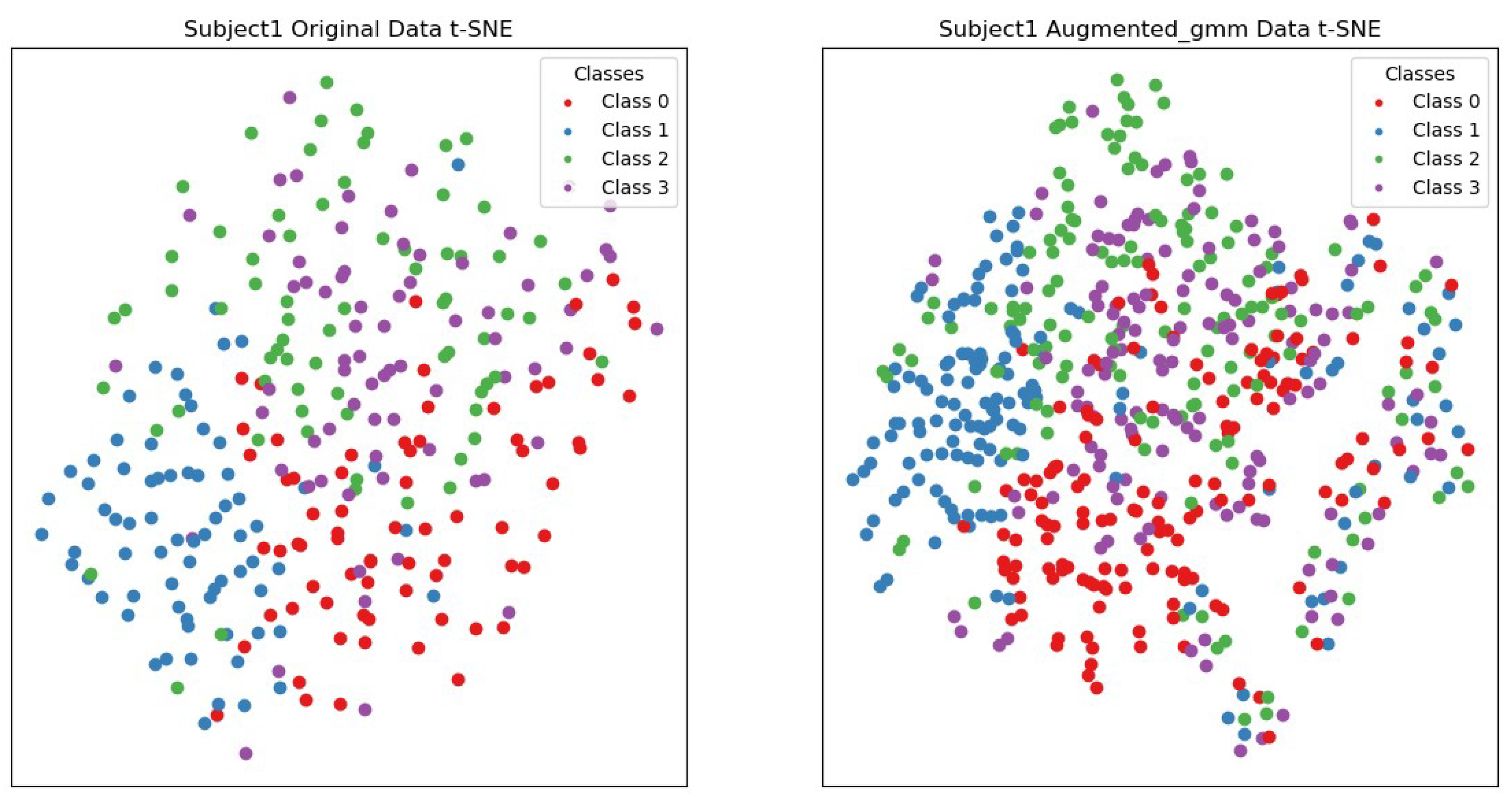
As shown in Figure 11, by comparing the t-SNE visualization of the original data and the data generated by augmentation methods for the first participant, we found that:
Figure 11.
t-SNE visualization of Subject 1’s original data and the data augmented using the Gaussian Mixture Model (GMM).Red represents the data for left-hand motor imagery, blue represents the data for right-hand motor imagery, green represents the data for both feet motor imagery, and purple represents the data for tongue motor imagery.
3.3.1. Clarity of Clusters
Original Data: In the t-SNE visualization of the original data, points from different classes do not have clear boundaries, leading to insufficient distinction between classes.
Augmentation Data: The data processed by the augmentation method described in this paper shows clearer cluster structures in t-SNE visualization. Points from each category are relatively clustered together, forming distinct clusters with certain boundaries between them. This indicates that the augmentation method effectively improves the distinguishability between different categories.
3.3.2. Local Structure Compactness
Original Data: In the t-SNE visualization of the original data, points from the same class are more dispersed and do not form tight clusters.
Augmentation Data: The data processed by the augmentation method described in this paper exhibits higher local structural compactness in t-SNE visualization. Points from the same category are closely clustered together, forming more compact clusters. This indicates that the augmentation method effectively improves the intra-class consistency.
In summary, the augmentation methods in this paper improve the visualization of the data, making points from different classes more clearly clustered together, and increasing the separation between different classes. This improvement helps enhance the performance of subsequent machine learning models, as clearer class boundaries and higher local structure compactness aid the model in learning and classifying data more accurately.
4. Discussion
The purpose of data augmentation is to improve the generalization ability of models by increasing data diversity, reduce overfitting, and ultimately enhance model performance on unseen data. Different augmentation methods can have varying impacts on model performance. In practical applications, the choice of which augmentation method to use depends on the specific classification task and objectives. Ideally, the specific impact of different augmentation methods on model performance should be evaluated through techniques such as cross-validation.
Based on the comparison of different augmentation methods and their effects on classification models discussed above, we can conclude:
(1) The method proposed in this paper demonstrates significant improvements across all models, particularly on FBCSP and Deep4Net, where the enhancements are most substantial, with increases of 11.92% and 29.84%, respectively. This indicates that the proposed method is an effective data augmentation technique that can significantly improve the generalization ability of models.
(2) Noise injection also shows considerable improvement on most models, especially on LSTM and ShallowNet, where the enhancement exceeds 30%, demonstrating the potential of noise addition in improving model robustness. However, the level of noise needs careful tuning to avoid obscuring useful information within the signal.
(3) Data expansion is beneficial for all types of models, especially for deep learning models that require large amounts of data to optimize parameters, as it can significantly improve the statistical performance of models and reduce overfitting.
(4) Combining multiple augmentation methods generally provides the best performance enhancement, but care must be taken to avoid excessive augmentation that may distort the signal, thereby reducing model performance. Therefore, the selection of augmentation methods and models needs to be carefully adjusted based on the characteristics of the data and the requirements of the task.
5. Conclusions
In this paper, we introduce an augmentation scheme based on Gaussian microstate feature reconstruction for EEG data to address issues related to the disruption of spatiotemporal dynamic features or reliance on a large number of real samples. The scheme involves Gaussian clustering of similar samples to extract mixed representations of microstates, followed by exchanging and reconstructing new Gaussian mixture model probability features based on the similarity of probability features between two samples of the same type. New sample data is generated through sampling based on probability, mean, and variance. Its performance was tested and evaluated on datasets. Experimental results demonstrate that our proposed scheme is an effective data augmentation technique in terms of motor imagery recognition accuracy, significantly enhancing the generalization ability of models.
6. Results
This section may be divided by subheadings. It should provide a concise and precise description of the experimental results, their interpretation as well as the experimental conclusions that can be drawn.
Author Contributions
Conceptualization, Z.J. and L.C.; methodology, L.C. and Z.S.; software, L.C.; validation, Z.S.,L.C. and W.C.; formal analysis, L.Y.; investigation, Z.S.; resources, Z.J.; data curation, Z.S.; writing—original draft preparation, L.C.; writing—review and editing, L.C.; visualization, L.C.and W.C.; supervision, Z.J.and W.X.; project administration, Z.J.; funding acquisition, Z.J. All authors have read and agreed to the published version of the manuscript.
Funding
This work is funded by the Special Fund for Research on National Major Research Instruments (62227801) of the Nature Science Foundation of China.
Data Availability Statement
To substantiate the uniqueness of my research, I have made the preliminary data and code snippets (if applicable) from this manuscript, along with my article published in September, publicly available on the respective websites.https://github.com/liaoliao3450/EEG-Data-Augmentation-Method: EEG Data Augmentation Method Based on the Gaussian Mixture Model.
Conflicts of Interest
The authors declare no conflicts of interest.
Abbreviations
The following abbreviations are used in this manuscript:
| EEG | Electroencephalograms |
| GNAs | Generative Adversarial Networks |
| VAEs | Ariational Autoencoders |
| SNR | Signal-to-noise Ratio |
| GMM | Gaussian Mixture Models |
References
- Abdul Hussain, A.; Singh, A.; Guesgen, H.; Lal, S. A Comprehensive Review on Critical Issues and Possible Solutions of Motor Imagery Based Electroencephalography Brain-Computer Interface. Sensors 2021, 21. [Google Scholar] [CrossRef]
- Roy, Y.; Banville, H.; Albuquerque, I.; Gramfort, A.; Falk, T.H.; Faubert, J. Deep learning-based electroencephalography analysis: a systematic review. Journal of Neural Engineering 2019, 16, 051001. [Google Scholar] [CrossRef]
- Bigdely-Shamlo, N.; Mullen, T.; Kothe, C.; Su, K.M.; Robbins, K.A. The PREP pipeline: standardized preprocessing for large-scale EEG analysis. Frontiers in Neuroinformatics 2015, 9. [Google Scholar] [CrossRef]
- Jas, M.; Engemann, D.A.; Bekhti, Y.; Raimondo, F.; Gramfort, A. Autoreject: Automated artifact rejection for MEG and EEG data. NeuroImage 2017, 159, 417–429. [Google Scholar] [CrossRef] [PubMed]
- Gramfort, A.; e, D.S.; Haueisen, J.; Hämäläinen, M.; Kowalskig, M. Time-frequency mixed-norm estimates: Sparse M/EEG imaging with non-stationary source activations. NeuroImage 2013, 70, 410–422. [Google Scholar] [CrossRef]
- Kuanar, S.; Athitsos, V.; Pradhan, N.; Mishra, A.; Rao, K. Cognitive Analysis of Working Memory Load from Eeg, by a Deep Recurrent Neural Network. In Proceedings of the 2018 IEEE International Conference on Acoustics, Speech and Signal Processing (ICASSP); 2018; pp. 2576–2580. [Google Scholar] [CrossRef]
- Gramfort, A.; Strohmeier, D.; J. Haueisen e, f.; d, M.H.; g, M.K. Brain–machine interfaces from motor to mood. Nature Neuroscience 2019, 22, 1554–1564. [CrossRef] [PubMed]
- Sani1, O.; Yang1, Y.; Lee1, M.; Dawes2, H.; Chang2, E.; Shanechi1, M. Neural Decoding and Control of Mood to Treat Neuropsychiatric Disorders. Biological Psychiatry 2020, 87, s95–s96. [Google Scholar] [CrossRef]
- Sakai, A.; Minoda, Y.; Morikawa, K. Data augmentation methods for machine-learning-based classification of bio-signals. In Proceedings of the 2017 10th Biomedical Engineering International Conference (BMEiCON); 2017; pp. 1–4. [Google Scholar] [CrossRef]
- Krell, M.M.; Kim, S.K. Rotational data augmentation for electroencephalographic data. In Proceedings of the 2017 39th Annual International Conference of the IEEE Engineering in Medicine and Biology Society (EMBC); 2017; pp. 471–474. [Google Scholar] [CrossRef]
- Lashgari, E.; Liang, D.; Maoz, U. Data augmentation for deep-learning-based electroencephalography. Journal of Neuroscience Methods 2020, 346, 108885. [Google Scholar] [CrossRef] [PubMed]
- Um, T.T.; Pfister, F.M.J.; Pichler, D.; Endo, S.; Lang, M.; Hirche, S.; Fietzek, U.; Kulić, D. Data augmentation of wearable sensor data for parkinson’s disease monitoring using convolutional neural networks. In Proceedings of the Proceedings of the 19th ACM International Conference on Multimodal Interaction, New York, NY, USA, 2017; ICMI ’17, p. 216–220. [CrossRef]
- Lotte.; Fabien. Signal Processing Approaches to Minimize or Suppress Calibration Time in Oscillatory Activity-Based Brain–Computer Interfaces. Proceedings of the IEEE 2015, 103, 871–890. [CrossRef]
- Pei, Y.; Luo, Z.; Yan, Y.; Yan, H.; Jiang, J.; Li, W.; Xie, L.; Yin, E. Data Augmentation: Using Channel-Level Recombination to Improve Classification Performance for Motor Imagery EEG. Proceedings of the IEEE 2021, 15, 645–952. [Google Scholar] [CrossRef]
- Kim, S.J.; Lee, D.H.; Choi, Y.W. CropCat: Data Augmentation for Smoothing the Feature Distribution of EEG Signals. In Proceedings of the 2023 11th International Winter Conference on Brain-Computer Interface (BCI); 2023; pp. 1–4. [Google Scholar] [CrossRef]
- Y, L.; LZ, Z.; ZY, W.; BL, L. Data augmentation for enhancing EEG-based emotion recognition with deep generative models. Journal of neural engineering 2020, 17. [Google Scholar] [CrossRef]
- Schwabedal, J.T.C.; Snyder, J.C.; Cakmak, A.; Nemati, S.; Clifford, G.D. Addressing Class Imbalance in Classification Problems of Noisy Signals by using Fourier Transform Surrogates. ArXiv, 2018; 1–8. [Google Scholar] [CrossRef]
- Rommel, C.; Moreau, T.; Gramfort, A. CADDA: Class-wise Automatic Differentiable Data Augmentation for EEG Signals. ArXiv, 2021; abs/2106.13695. [Google Scholar]
- Deiss, O.; Biswal, S.; Jing, J.; Sun, H.; Westover, M.B.; Sun, J. HAMLET: Interpretable Human And Machine co-LEarning Technique. ArXiv 2018, 238–253. [Google Scholar] [CrossRef]
- Saeed, A.; Grangier, D.; Pietquin, O.; Zeghidour, N. Learning From Heterogeneous Eeg Signals with Differentiable Channel Reordering. In Proceedings of the ICASSP 2021 - 2021 IEEE International Conference on Acoustics, Speech and Signal Processing (ICASSP); 2021; pp. 1255–1259. [Google Scholar] [CrossRef]
- Chawla, N.V.; Bowyer, K.W.; Hall, L.O.; Kegelmeyer, W.P. SMOTE: synthetic minority over-sampling technique. J. Artif. Int. Res. 2002, 16, 321–357. [Google Scholar] [CrossRef]
- Wang, F.; Zhong, S.h.; Peng, J.; Jiang, J.; Liu, Y. Data Augmentation for EEG-Based Emotion Recognition with Deep Convolutional Neural Networks. In Proceedings of the MultiMedia Modeling, Cham; 2018; pp. 82–93. [Google Scholar] [CrossRef]
- Mohsenvand, M.N.; Izadi, M.R.; Maes, P. Contrastive Representation Learning for Electroencephalogram Classification. In Proceedings of the Proceedings of the Machine Learning for Health NeurIPSWorkshop; Alsentzer, E.; McDermott, M.B.A.; Falck, F.; Sarkar, S.K.; Roy, S.; Hyland, S.L., Eds. PMLR, 11 Dec 2020, Vol. 136, Proceedings of Machine Learning Research, pp. 238–253.
- Pan, S.J.; Yang, Q. A Survey on Transfer Learning. IEEE Transactions on Knowledge and Data Engineering 2010, 22, 1345–1359. [Google Scholar] [CrossRef]
- Li, Y.; Huang, J.; Zhou, H.; Zhong, N. Human Emotion Recognition with Electroencephalographic Multidimensional Features by Hybrid Deep Neural Networks. Applied Sciences 2017, 7. [Google Scholar] [CrossRef]
- Fu, R.; Wang, Y.; Jia, C. A new data augmentation method for EEG features based on the hybrid model of broad-deep networks. Expert Systems with Applications 2022, 202, 117386. [Google Scholar] [CrossRef]
- Arjovsky, M.; Chintala, S.; Bottou, L. Wasserstein generative adversarial networks. In Proceedings of the Proceedings of the 34th International Conference on Machine Learning - Volume 70. JMLR.org, 2017, ICML’17, p. 214–223. [CrossRef]
- Gulrajani, I.; Ahmed, F.; Arjovsky, M.; Dumoulin, V.; Courville, A. Improved training of wasserstein GANs. In Proceedings of the Proceedings of the 31st International Conference on Neural Information Processing Systems, Red Hook, NY, USA, 2017; NIPS’17, p. 5769–5779. [CrossRef]
- Mao, X.; Li, Q.; Xie, H.; Lau, R.Y.; Wang, Z.; Smolley, S.P. Least Squares Generative Adversarial Networks. In Proceedings of the 2017 IEEE International Conference on Computer Vision (ICCV); 2017; pp. 2813–2821. [Google Scholar] [CrossRef]
- Hartmann, K.G.; Schirrmeister, R.T.; Ball, T. EEG-GAN: Generative adversarial networks for electroencephalograhic (EEG) brain signals. ArXiv 2018. [Google Scholar] [CrossRef]
- Luo, Y.; Lu, B.L. EEG Data Augmentation for Emotion Recognition Using a Conditional Wasserstein GAN. In Proceedings of the 2018 40th Annual International Conference of the IEEE Engineering in Medicine and Biology Society (EMBC); 2018; pp. 2535–2538. [Google Scholar] [CrossRef]
- Fahimi, F.; Dosen, S.; Ang, K.K.; Mrachacz-Kersting, N.; Guan, C. Generative Adversarial Networks-Based Data Augmentation for Brain–Computer Interface. IEEE Transactions on Neural Networks and Learning Systems 2021, 32, 4039–4051. [Google Scholar] [CrossRef] [PubMed]
- Ramponi, G.; Protopapas, P.; Brambilla, M.; Janssen, R. T-CGAN: Conditional Generative Adversarial Network for Data Augmentationin Noisy Time Series with Irregular Sampling. CoRR, 2018; abs/1811.08295. [Google Scholar]
- JOUR. ; Fei, Z.; Fei, Y.; Yuchen, F.; Quan, L.; Bairong, S. Electrocardiogram generation with a bidirectional LSTM-CNN generative adversarial network. Scientific Reports 2019, 9. [Google Scholar] [CrossRef]
- Bao, G.; Yan, B.; Tong, L.; Shu, J.; Wang, L.; Yang, K.; Zeng, Y. Data Augmentation for EEG-Based Emotion Recognition Using Generative Adversarial Networks. Frontiers in Computational Neuroscience 2021, 15. [Google Scholar] [CrossRef]
- Tait, L.; Zhang, J. MEG cortical microstates: Spatiotemporal characteristics, dynamic functional connectivity and stimulus-evoked responses. NeuroImage 2022, 251, 119006. [Google Scholar] [CrossRef] [PubMed]
- Liu, W.; Liu, X.; Dai, R.; Tang, X. Exploring differences between left and right hand motor imagery via spatio-temporal EEG microstate. Computer Assisted Surgery 2017, 22, 258–266. [Google Scholar] [CrossRef] [PubMed]
- Blanchard, G.; Blankertz, B. BCI Competition 2003–Data set IIa: spatial patterns of self-controlled brain rhythm modulations. IEEE Trans Biomed Eng 2004, 51, 1062–1066. [Google Scholar] [CrossRef] [PubMed]
- Liao, C.; Zhao, S.; Zhang, J. Motor Imagery Recognition Based on GMM-JCSFE Model. IEEE Transactions on Neural Systems and Rehabilitation Engineering 2024, 32, 3348–3357. [Google Scholar] [CrossRef]
- Ang, K.K.; Chin, Z.Y.; Wang, C.; Guan, C.; Zhang, H. Filter Bank Common Spatial Pattern Algorithm on BCI Competition IV Datasets 2a and 2b. Frontiers in Neuroscience 2012, 6. [Google Scholar] [CrossRef] [PubMed]
- Hochreiter, S.; Schmidhuber, J. Long Short-Term Memory. Neural Computation 1997, 9, 1735–1780. [Google Scholar] [CrossRef] [PubMed]
- Lawhern, V.J.; Solon, A.J.; Waytowich, N.R.; Gordon, S.M.; Hung, C.P.; Lance, B.J. EEGNet: a compact convolutional neural network for EEG-based brain–computer interfaces. Journal of Neural Engineering 2018, 15, 056013. [Google Scholar] [CrossRef]
- Xingfei, H.; Deyang, W.; Haiyan, L.; Fei, J.; Hongtao, L. ShallowNet: An Efficient Lightweight Text Detection Network Based on Instance Count-Aware Supervision Information. In Proceedings of the Neural Information Processing, Cham; 2021; pp. 633–644. [Google Scholar]
- Schirrmeister, R.; Gemein, L.; Eggensperger, K.; Hutter, F.; Ball, T. Deep learning with convolutional neural networks for decoding and visualization of EEG pathology. In Proceedings of the 2017 IEEE Signal Processing in Medicine and Biology Symposium (SPMB); 2017; pp. 1–7. [Google Scholar] [CrossRef]
Figure 1.
Principle diagram of EEG microstate analysis.
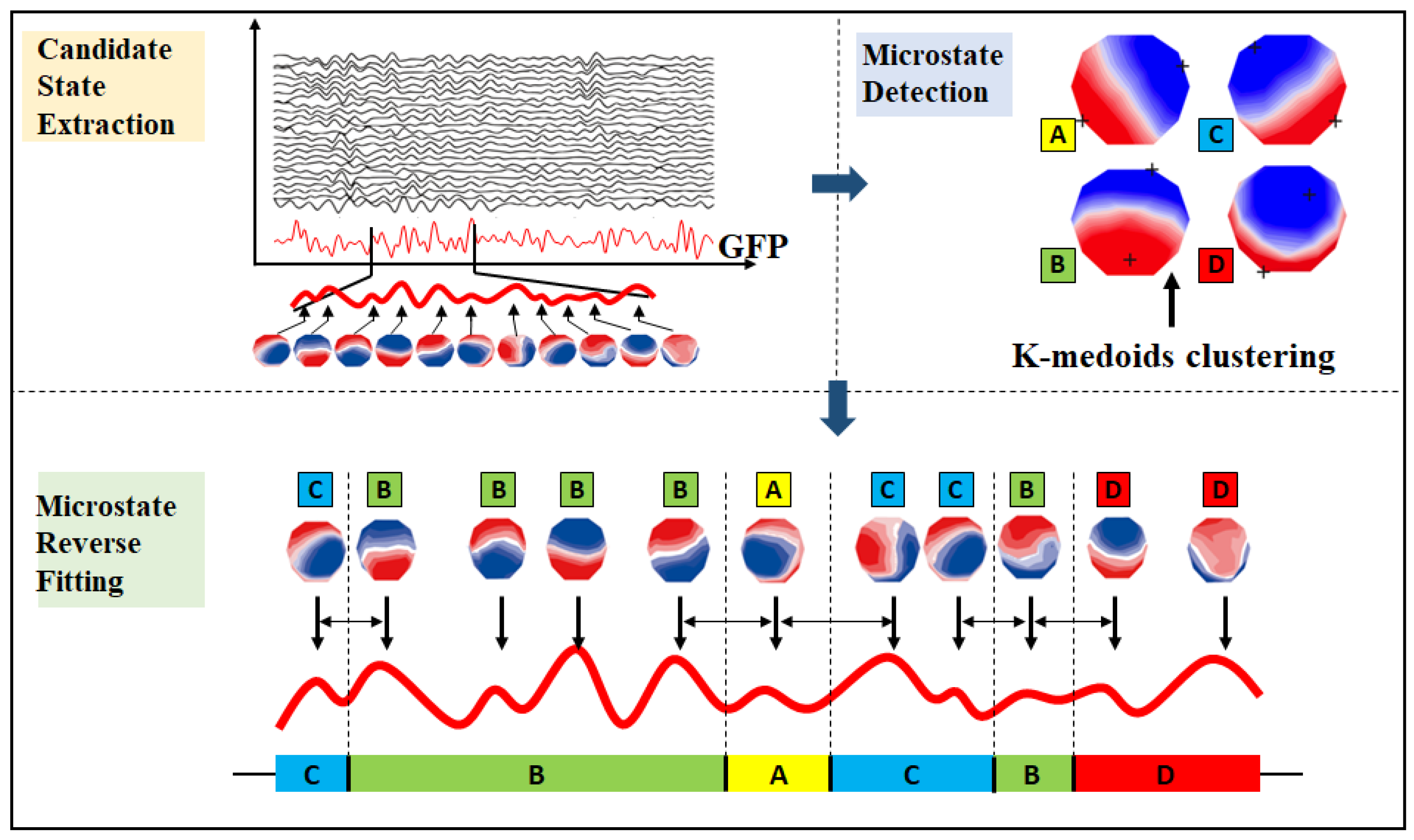
Figure 2.
Feature extraction of microstate hybrid model based on GMM.
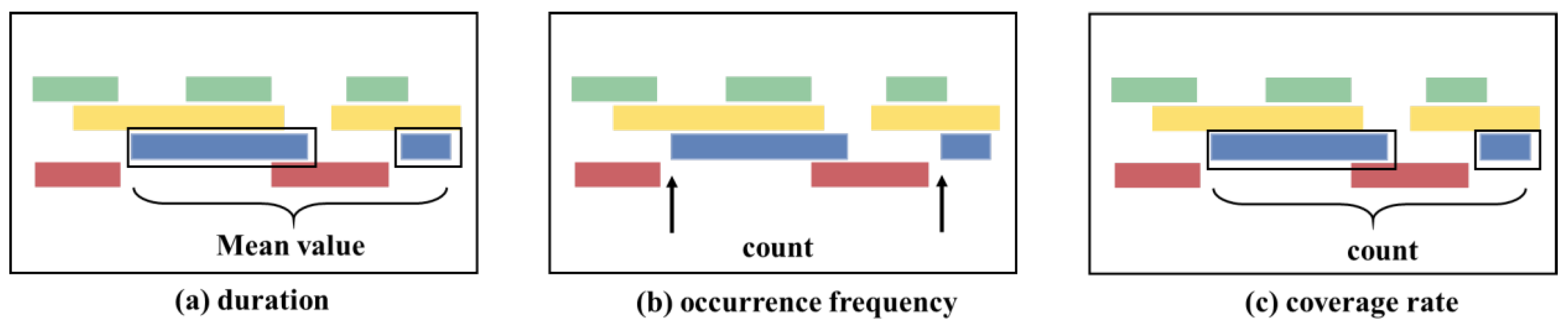
Figure 3.
Principle diagram of the EEG data augmentation method based on Gaussian mixture models.Data preprocessing mainly includes filtering(0-38HZ), segmentation and baseline correction, removing artifacts, and referencing. (a) Decomposition.First, preprocess the original EEG data, then use the Gaussian Mixture Model (GMM) for clustering. Calculate the product matrix of weights and probabilities for adjacent data points with the same label. Swap points with similarity coefficients greater than a threshold to obtain a new microstate feature matrix. (b) Reconstruction.First, set a random seed to ensure the reproducibility of results. For each sample, randomly select a channel, swap channels between the original data and the fitted data, and finally generate new EEG data.
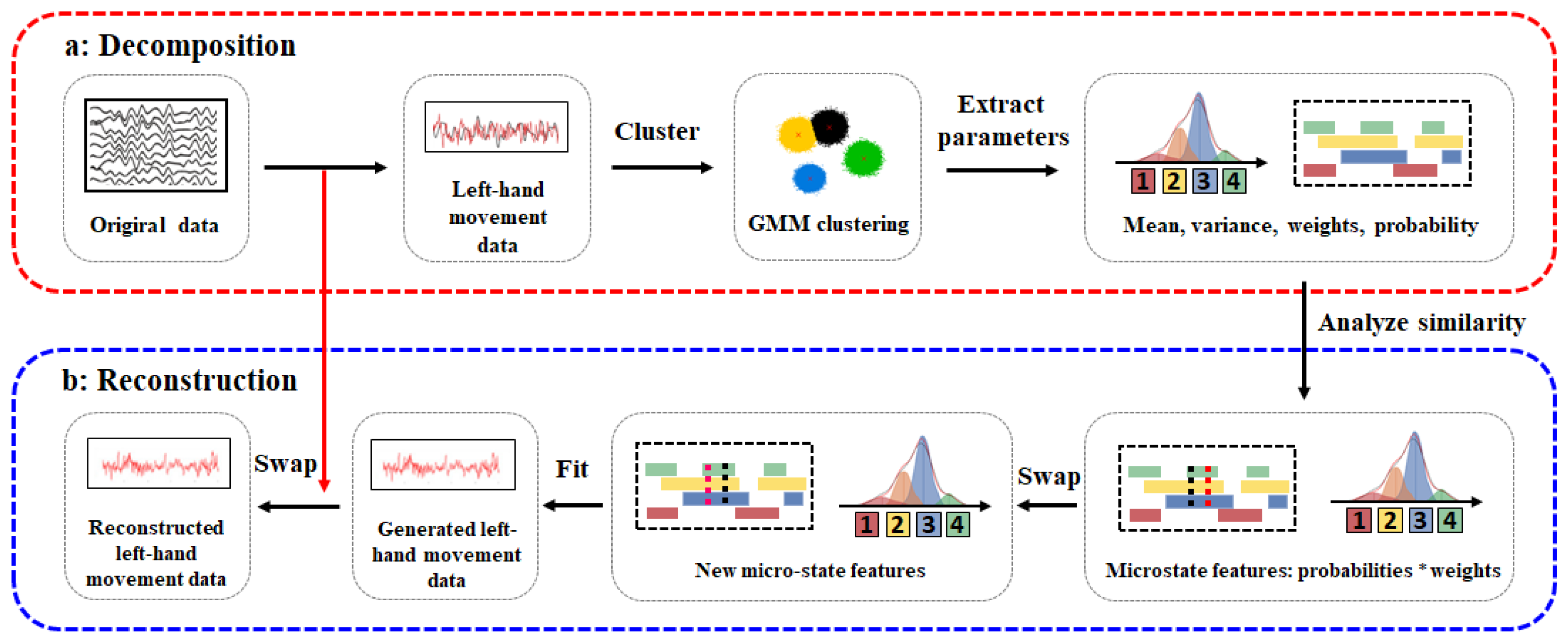

Table 1.
Algorithm Process for EEG Data Augmentation Method Based on Gaussian Mixture Model.
| Algorithm:EEG Data Augmentation Method Based on Gaussian Mixture Model |
|---|
| Input:original_data = (trial,channel,n_samples), original_labels =(trial,) |
| Output:gmm_data |
| Step1:Set model parameters.n_components = 10;random_stata = 42; = 0.8 |
| Step2:Cluster the data with the same label and calculate the microstate features |
| of each sample belonging to each cluster. |
| probs = gmm.predict_proba(original_data) |
| means = gmm.means_ |
| covariances = gmm. covariances_ |
| weights =gmm.weights_robs |
| Step3:Sampling. |
| for do |
| for do |
| for do |
| end |
| end |
| end |
| Step4:Calculate the product matrix. |
| weighted_probs_values = gmm.weights_ * probs |
| Step5:Swap similar points. |
| weighted_probs_values = swap_columns(weighted_probs_values, ) |
| Step6:Fit the data. |
| data_generate_sampel = np.matmul(weighted_probs_values ,fitted_values) |
| Step7:Swap channels and reconstruct the data. |
| gmm_data = GMM_FEATURE(probability=probability,random_state=42) |
Table 2.
Comparison of average classification accuracy in K-fold cross-validation between data generated by different augmentation methods and the original data accuracy mean on dataset .
Table 2.
Comparison of average classification accuracy in K-fold cross-validation between data generated by different augmentation methods and the original data accuracy mean on dataset .
| Method | FBCSP [40] | LSTM [41] | EEGNet [42] | ShallNet [43] | Deep4Net [44] | Avg | SD |
|---|---|---|---|---|---|---|---|
| Original data | 67.75 | 48.17 | 46.07 | 48.91 | 52.89 | 52.76 | 8.74 |
| Noise Addition | 73.22 | 80.72 | 75.29 | 80.32 | 83.08 | 78.53 | 4.10 |
| Sign Flip | 74.63 | 80.72 | 74.50 | 81.84 | 82.75 | 78.89 | 4.01 |
| Time reverse | 78.27 | 79.32 | 76.39 | 79.73 | 79.90 | 78.72 | 1.45 |
| Time Masking | 75.46 | 79.88 | 75.52 | 80.17 | 80.92 | 78.39 | 2.67 |
| FT Surrogate | 81.26 | 77.60 | 73.34 | 80.13 | 82.19 | 78.90 | 3.55 |
| Frequency Shift | 81.18 | 74.40 | 68.47 | 72.79 | 76.83 | 74.73 | 4.72 |
| Bandstop fliter | 76.32 | 78.39 | 76.98 | 78.16 | 81.13 | 78.20 | 1.85 |
| Channel Sym | 77.87 | 75.86 | 73.93 | 79.47 | 81.61 | 77.75 | 3.00 |
| Channel Shuffle | 78.59 | 76.51 | 68.29 | 75.06 | 79.86 | 75.66 | 4.52 |
| GMM Aug | 79.67 | 80.53 | 77.70 | 82.61 | 82.73 | 80.64 | 2.11 |
Disclaimer/Publisher’s Note: The statements, opinions and data contained in all publications are solely those of the individual author(s) and contributor(s) and not of MDPI and/or the editor(s). MDPI and/or the editor(s) disclaim responsibility for any injury to people or property resulting from any ideas, methods, instructions or products referred to in the content. |
© 2025 by the authors. Licensee MDPI, Basel, Switzerland. This article is an open access article distributed under the terms and conditions of the Creative Commons Attribution (CC BY) license (http://creativecommons.org/licenses/by/4.0/).
Copyright: This open access article is published under a Creative Commons CC BY 4.0 license, which permit the free download, distribution, and reuse, provided that the author and preprint are cited in any reuse.


