
Submitted:
21 January 2025
Posted:
22 January 2025
Read the latest preprint version here
Abstract
Hellenic Open University has developed Onlabs, a virtual biology laboratory designed to safely and effectively prepare its students for hands-on work in the university’s on-site labs. This platform simulates key experimental processes, such as 10x TBE solution preparation, agarose gel preparation and electrophoresis, which involve liquid transfers between bottles. However, accurately depicting liquid volumes within complex-shaped laboratory vessels, such as Erlenmeyer flasks and burettes, remains a challenge. This paper addresses this limitation by introducing a unified parametric framework for modeling circular cross-section pipes, including straight pipes with constant diameter, curved pipes with constant diameter and straight conical pipes. Analytical expressions are developed to define the position and orientation of points along a pipe's central axis, as well as the surface geometry of composite pipes formed by combining these elements in planar configurations. The primary goal is to enable the precise algorithmic generation of 3D graphics representing the surfaces of liquids within various laboratory vessels. By leveraging these parametric models, liquid volumes can be accurately visualized, reflecting the vessels’ geometries and improving the realism of simulations.
Keywords:
Fluid Simulation
; Liquid Simulation
; Virtual Labs
; Virtual Reality
1. Introduction
One of the most challenging tasks faced by science universities is ensuring effective instruction and assessment of students in using laboratory equipment and conducting experiments successfully. On-site laboratory use is accompanied by serious risks, including the potential for accidents and equipment damage. These risks often limit the extent to which students can engage in hands-on practice and experimentation, thereby restricting opportunities for learning through trial and error. Additionally, distance learning universities that provide science education encounter an added difficulty: their students are rarely, if ever, physically present at laboratory facilities, making lab-based training and evaluation even more complex.
Virtual laboratories have emerged as a promising solution to complement traditional on-site lab training. These platforms allow students to gain familiarity with specialized equipment and experimental procedures in a safe and controlled environment. Within a virtual lab, users can interact with instruments and perform experiments as often as needed, free from the fear of accidents or equipment damage. Furthermore, these platforms provide a means of evaluating students’ performance. Assessment can be carried out either by a supervising human expert or through automated evaluation tools embedded within the virtual lab software.
This dual necessity and ambition have driven the Hellenic Open University (HOU) to develop Onlabs, a 3D virtual biology laboratory designed for remote training and evaluation of undergraduate and postgraduate students in the natural sciences. The fundamental idea behind Onlabs is that students can practice and refine their laboratory skills at home, using the software, before handling actual equipment in an on-site lab setting.
1.1. About Onlabs Virtual Lab
In contrast to traditional on-site training, Onlabs allows students to experiment freely with laboratory instruments and equipment in virtually unlimited ways. They can even intentionally or unintentionally misuse equipment and learn from their mistakes without real-world consequences.
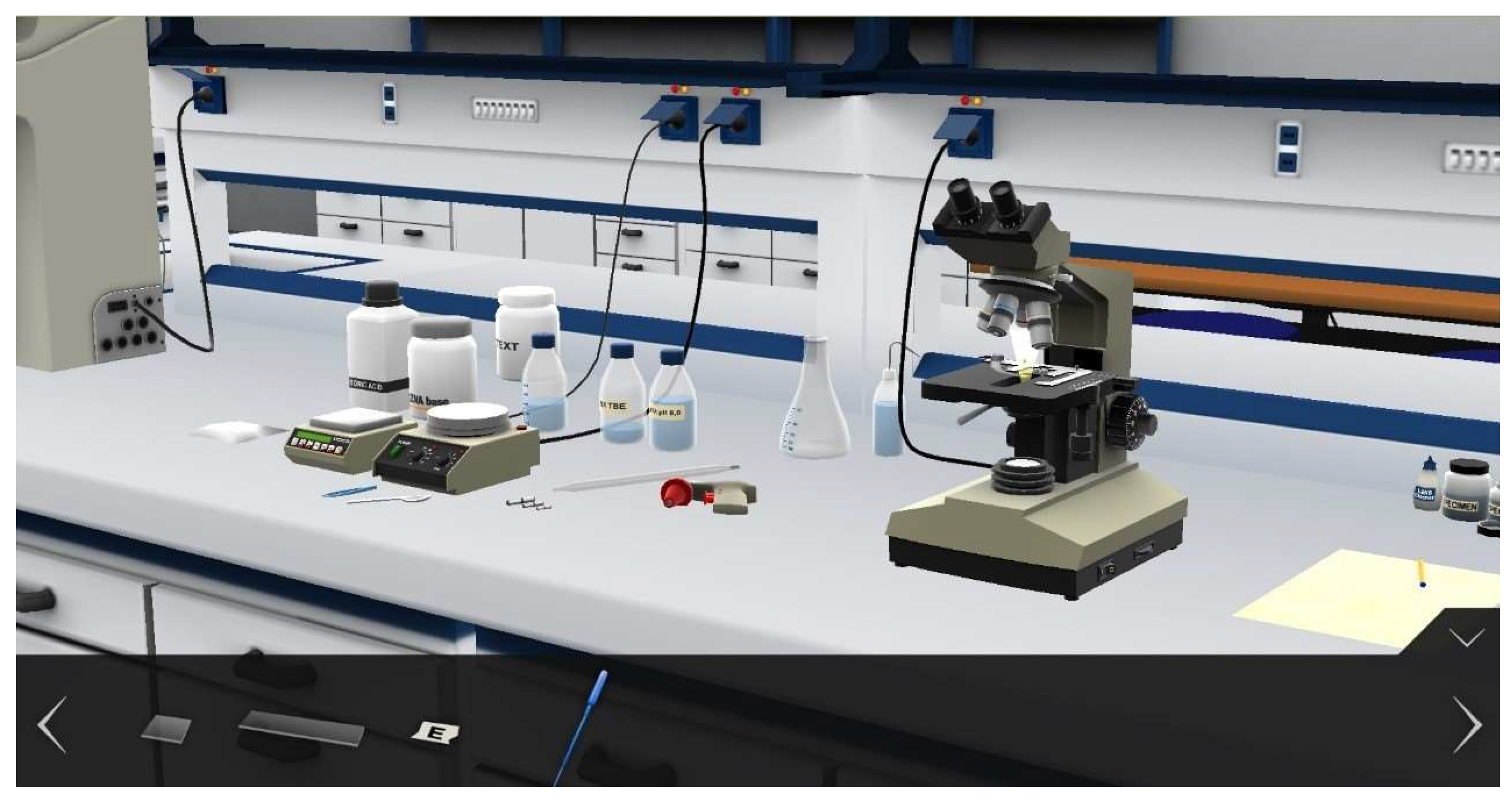
Onlabs is designed to simulate the experience of a computer game, incorporating state-of-the-art 3D graphics and interactive elements. Users can navigate the environment using a mouse and keyboard, manipulate objects, turn knobs, click switches, and more (Figure 1).
Initially, Onlabs was developed using Hive3D (https://www.eyelead.com/). However, since 2016, its development has transitioned to Unity. A variety of Onlabs versions are available on our website (http://onlabs.eap.gr/), ranging from stable releases to research prototypes. The most recent stable version (version 2.1.2) includes two distinct simulated experimental procedures: microscoping and the preparation of a 10X TBE solution. It also features three distinct play modes: instruction, experimentation, and evaluation.
In the microscoping experiment, users are required to set up a microscope, prepare a test specimen, and observe it using all objective lenses of a photonic microscope. Meanwhile, in the preparation of 500 mL of a 10X TBE solution, users measure out 17.4 grams of boric acid and 54 grams of Trizma base on an electronic scale, dissolve these powders in water using a magnetic stirrer, and then add additional water and EDTA pH 8.0 (ethylenediamine tetraacetic acid) to complete the solution.
The three play modes offer varying levels of guidance and freedom. In instruction mode, users follow voice and text prompts step by step, with the system only allowing the prescribed actions at each stage. Experimentation mode removes these restrictions, granting users full freedom to explore and perform any implemented actions. Finally, evaluation mode provides users with a numerical score reflecting how well they followed the experimental procedure and whether they successfully completed the simulation.
Onlabs version 3.0 beta introduces two updated experimental procedures that replace those in version 2.1.2. These include microscoping, as featured in previous versions, and electrophoresis, which begins with includes 500 mL of 10X TBE water solution as its first step.
For Onlabs’s conceptual design, implementation but also its evaluation by students with respect to its educational value, the reader may refer to previous publications of ours (cited on our website).
1.2. Liquid Simulation in Onlabs
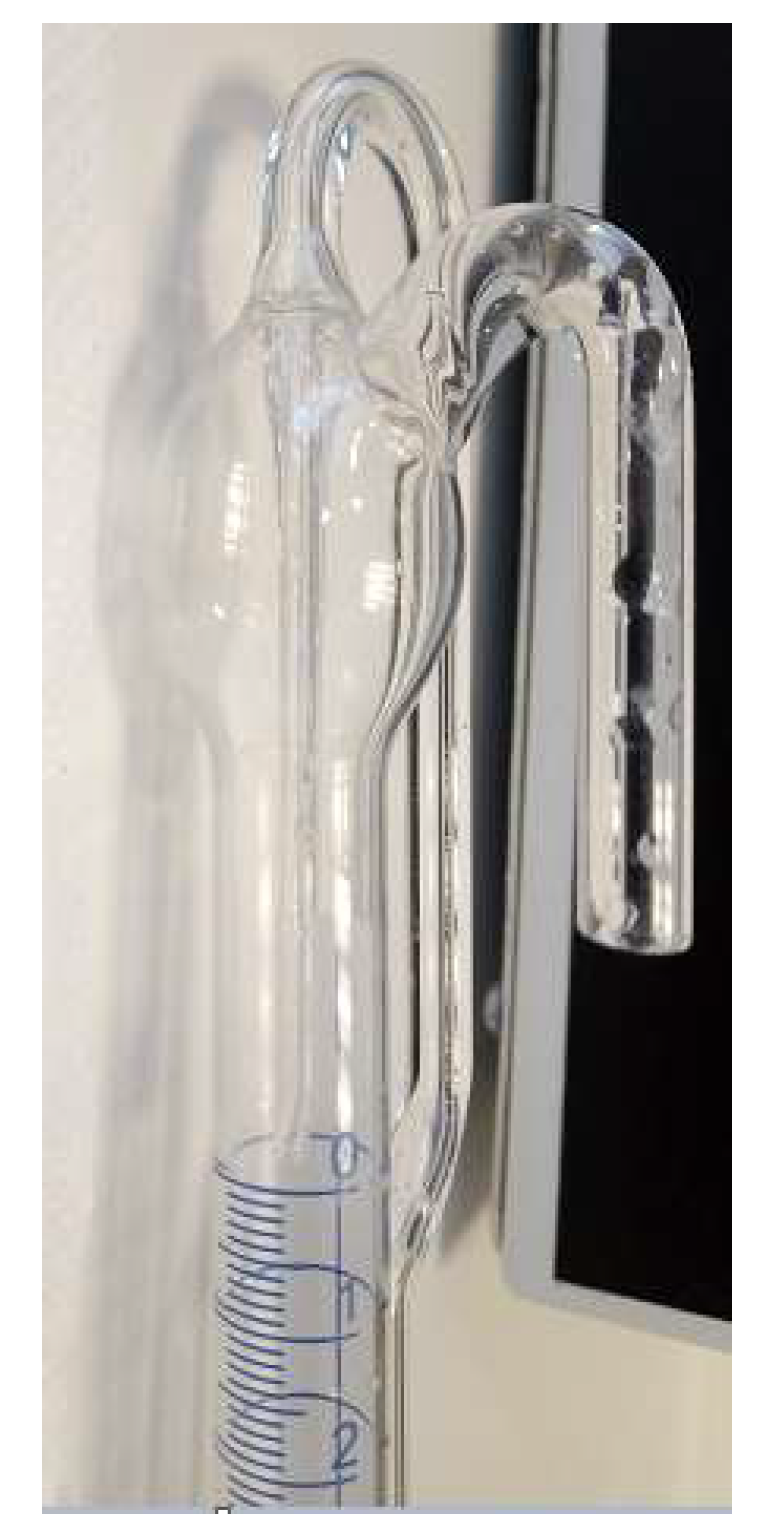
For experimental procedures such as the afore-mentioned ones of 10X TBE water solution preparation and electrophoresis, vessels of various forms are involved, such as conical flasks, being wide-necked or not, and volumetric tubes, as shown in Figures Figure 2, Figure 3 and Figure 4. Moreover, in other procedures mainly performed in a Chemistry lab, such as the determination of the rate constant of methyl acetate hydrolysis in the presence of acid, more perplexed vessels are used, like burettes, consisting of several different pipe segments being straight or curved (Figures Figure 5 and Figure 6).
Figure 2.
Conical flask.
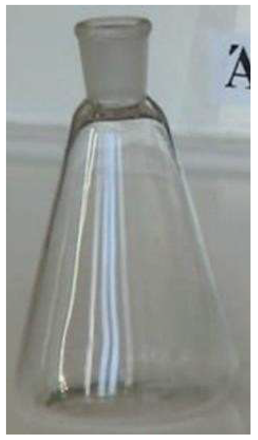
Figure 3.
Wide-necked conical flask.
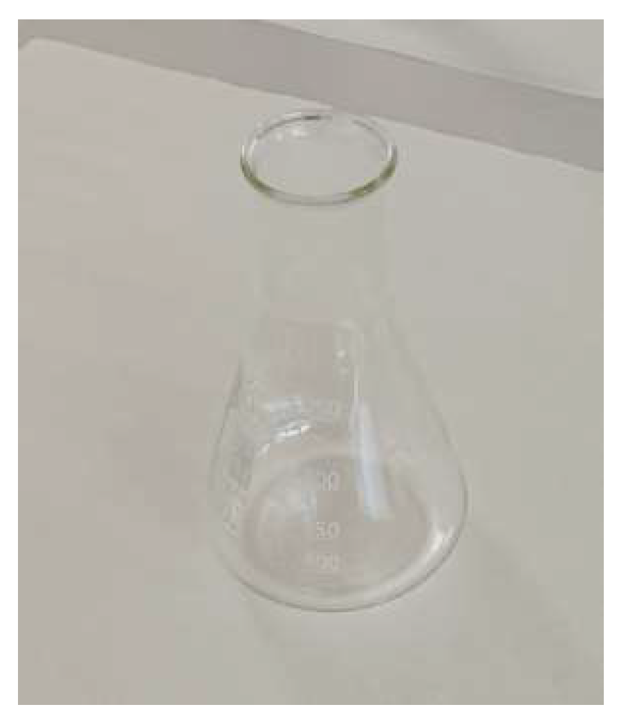
Figure 4.
Volumetric tube.
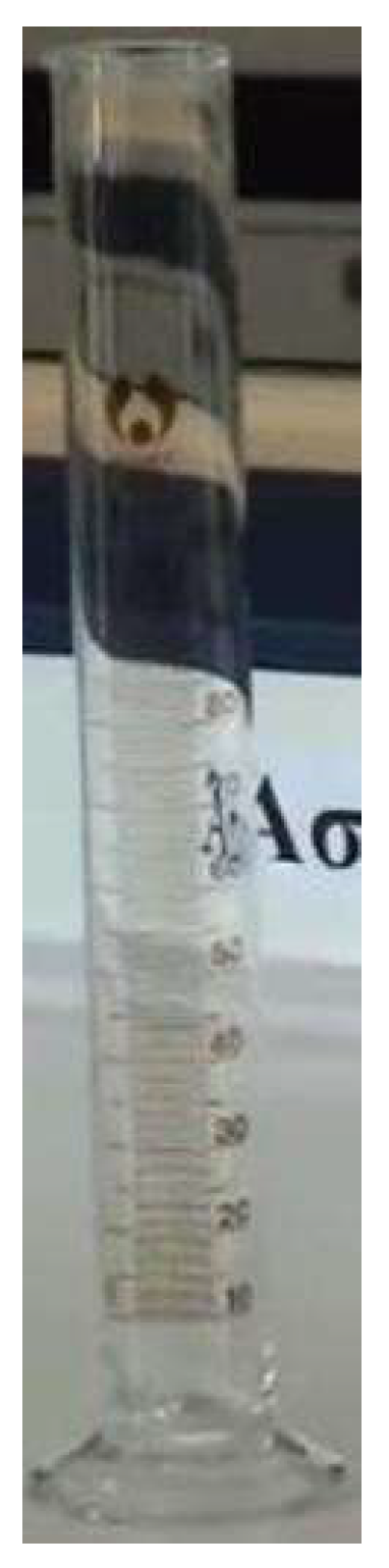
Figure 5.
Burette.
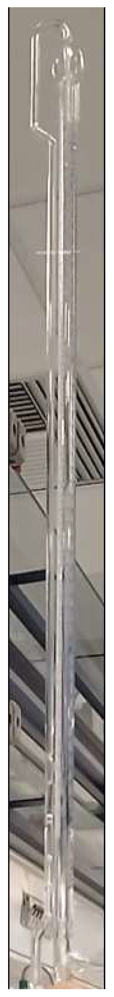
Figure 6.
Detailed view of burette’s curved pipe.
For those complex vessels, the dynamic creation in Unity (or any other 3D game engine) of the meshes corresponding to the interior liquids is obviously not an easy task. Our first technique presented in this paper tackles this problem efficiently with the use of advanced analytical geometry in the 3D space. Based on the afore-mentioned method of liquid simulation, we afterwards present a second technique which deals with the simulation of liquid transfer between the lab vessels of various shapes.
2. Background & Related Work
Over the years, various companies have made significant strides in creating interactive 3D virtual laboratories designed specifically for chemistry and biology education. These virtual labs are characterized by their incorporation of advanced graphics and cutting-edge visual effects, aiming to provide users with an immersive and engaging experience. Among the most prominent examples in this field are Labster (https://www.labster.com/) and Learnexx 3D (http://virtualsciencelab.com/index.html). These platforms have gained widespread recognition and are extensively used as training tools for both university students and laboratory professionals. Their popularity stems from their ability to simulate experimental workflows in a visually appealing and user-friendly manner.
However, it is important to note that these platforms generally do not prioritize detailed quantitative simulations. Instead, they focus on guiding users through specific actions that produce predetermined outcomes. For example, these simulations might demonstrate how to fill a bottle to capacity or measure the exact amount of a powdered substance required for a given experiment. The primary educational objective of these tools is to familiarize users with the qualitative procedural steps needed to complete an experiment successfully. In this sense, the emphasis is placed on understanding the sequence of actions rather than on achieving precise quantitative results.
On the other hand, there exists another category of chemistry simulations that shifts the focus entirely toward quantitative accuracy and precision. These simulations emphasize tasks such as exact measurements, accurate titrations, and even the inclusion of background chemical reactions. A representative application of this kind is ChemCollective Virtual Labs (https://chemcollective.org/vlabs). However, while these simulations excel in quantitative realism, they fall short in other areas. Specifically, they are typically confined to two-dimensional environments and lack the interactive depth and visual sophistication found in the first group of virtual labs. Despite their limitations, the underlying chemistry principles required to develop these simulations can often be encoded into specialized computational engines with relative ease [1].
Our goal of quantitative chemistry simulations is to address the divide between these two distinct categories of applications. By merging the advanced 3D graphics and high-quality visual effects of the first group with the quantitative precision and accuracy of the second group, we aim to deliver a comprehensive solution that incorporates the best aspects of both approaches.
Our first attempt of quantitative liquid transfer simulation within Onlabs, implemented for version 2.1 and also used in later versions, was based on scaling. Particularly, in order to simulate the aspiration and discarding of liquids from or to a cylindrical vessel with instruments like the electronic and automatic pipettes, the height of the cylinder representing the liquid inside is being increased or respectively decreased, creating the illusion that the liquid level rises or drops. In case though of a conical vessel, the cone representing the liquid inside is being split pre-runtime into several truncated cones of equal volume and the latter are successively scaled in real-time [2]. While our method deals with most of the vessels in a biology lab, it does not cover vessels and containers with irregular shapes like the ones described in the introduction. For this reason, we have developed a significantly more advanced liquid transfer simulation technique which we will present in following sections, which in turn is based on the method for liquid surface representation also presented in this paper.
In general, achieving a realistic visual outcome in liquid simulations is a rather challenging task. One widely used technique in this domain is fluid animation, which has been extensively applied in commercial computer games. This approach leverages solutions to the complex 3D Navier-Stokes Equations for fluid dynamics, combined with advanced graphical techniques for visualizing fluids. The foundational work in this area was carried out by Foster and Metaxas [3], whose contributions were heavily influenced by earlier research conducted by Harlow and Wlech [4] in the field of computational fluid dynamics. Over time, numerous advancements have been made in fluid animation. For instance, Stam [5,6] introduced an unconditionally stable model capable of producing intricate, fluid-like flows by efficiently solving the Navier-Stokes Equations, enhancing this way the realism of this kind of simulations significantly.
Another technique frequently used for realistic liquid simulation involves particle systems, which were first conceptualized by Reeves [7]. Particle systems are a versatile method employed not only for simulating liquids but also for modeling other types of fluids. These systems have become a staple in modern 3D game engines such as Unity, where they are valued for their adaptability and effectiveness in creating visually compelling fluid simulations. Clavet et al. [8] developed a particle-based method for viscoelastic fluid simulation, with which they simulated, among others, splashing of paint, mud or rain drops on moving objects as well as water fountains and pouring liquids into vessels.
In a different fashion, Medvecký-Heretik used cellular automata in order to realistically simulate liquids within the context of interactive applications (games) while also achieving low memory consumption and maintaining high frame rates [9].
Despite the advancements and widespread use of these techniques, it is notable that neither fluid animation nor particle systems have been applied to liquid simulations in the context of virtual laboratories, particularly for quantitatively modeling liquid transfers. This absence is not surprising, given the considerable costs associated with these techniques, both in terms of development time and the computational resources required during runtime. Recognizing these challenges, Onlabs has adopted a different approach to liquid transfer simulation. This alternative method circumvents the limitations of traditional techniques, offering a more practical solution tailored to the unique needs of virtual laboratory environments.
3. Materials and Methods
In this section, we describe our full technique on liquid simulation in a virtual lab. First, in sections 3.1 and 3.2, we address the problem of simulating liquids inside various vessels of complex structure by leveraging advanced analytical geometry. Thereafter, in section ..., building on that liquid simulation method, we propose another method, which deals with the simulation of liquid transfer between laboratory vessels of various shapes. The results from both of those simulation methods’ implementation under Unity/C# are presented in section 4.
3.1. Description of Pipes and Bottles with Circular Cross-Sections and Liquid Volume Representation
During the experimental procedure for determining the rate constant of methyl acetate hydrolysis in the presence of an acid as well as in all experimental procedures in Biology and Chemistry laboratories, bottles of various sizes and shapes are extensively used. Instruments with tubes, which facilitate the flow of liquid from one bottle to another, are also employed.
In the experiment examined in this study, there is extensive use of and transfers between conical, cylindrical/volumetric bottles and burettes. Specifically, during the use of an automatic burette, the following processes occur:
- Liquid flow through a tube, bottle emptying, and volumetric tube filling with free-flow during the filling of the automatic burette’s volumetric tube.
- Liquid flow through a tube and bottle refilling with free-flow from the automatic burette during the zeroing of the volumetric tube’s measurement.
- Emptying of the volumetric tube with liquid flow into the spout tube of the automatic burette’s measurement tap.
From the above, the utility and significance of simulating liquid flows, as well as the filling and emptying of bottles with liquids, become evident for enhancing the sense of realism experienced by the student/user. To achieve this, the movement of the liquid as a function of time must be simulated, ensuring this function closely mirrors the actual quantitative and temporal behavior of liquid flow within a tube or bottle.
3.1.1. Types and Classification of Liquid Movement
Liquid movement can be broadly classified, based on the applications of interest, into the following categories:
- Steady liquid flow in a tube
- Transient liquid flow in a tube
- Filling and emptying of a bottle
This work seeks a unified mathematical approach to describing pipes and bottles, facilitating seamless implementation in Unity/C#. Specifically, the goal was to parameterize the description of an entire composite pipe, enabling straightforward modeling and simulation across consecutive pipe segments.
3.1.2. Simplifying Assumptions
The following simplifying assumptions were made for describing pipes and bottles:
- Pipes and bottles are assumed to have circular cross-sections only.
- A single parameter, s, is used along the entire length of the composite pipe to represent the current length of the line formed by the centers of the circular cross-sections (central line).
- The diameter is continuous along each pipe/bottle segment and remains consistent during transitions between segments (i.e., the diameter at the end of one segment equals the diameter at the start of the next).
- The slope of the central line relative to the horizontal plane is continuous at every point along the pipe and during transitions between segments.
- The diameter of an individual pipe/bottle remains constant or varies linearly as a function of its length.
- For pipes, the liquid surface level is considered perpendicular to the central line at every point.
- Only vertical bottles are considered.
- A common curvature parameter, κ, is used for each pipe segment.
- The radius of curvature of the central line must be greater than or at least equal to the pipe’s cross-sectional radius.
- The central line of the composite pipe lies within a plane.
Essentially, the aim is to determine the Equations describing the coordinates of any point along the central line in the plane and the pipe’s slope at that point. This enables drawing the corresponding liquid level at that specific point.
3.1.3. Central Line Coordinate Equations for Curved Pipes with Constant Diameter and Straight Pipes with Constant or Linearly Varying Diameter
Recall that a composite pipe consists of various segments, some straight and some curved. To position each segment of the composite pipe in the plane, we initially identify a single point—the starting point of the segment’s central line. Naturally, the endpoint of one segment serves as the starting point for the next, so only the initial points of consecutive segments need to be specified. For each starting point of a pipe segment’s central line, the parameters that must be measured or determined include its horizontal and vertical coordinates and the slope (angle) of the central line relative to the horizontal plane.
Once these three values (horizontal coordinate, vertical coordinate, and slope) are defined for the start of a pipe segment, they can be used to calculate corresponding values for any arbitrary point along that segment. This is the basis for fully defining the positioning of the segment in the plane.
Let’s assume that the horizontal coordinate, vertical coordinate, and slope at point A of the central line of a curved segment of the burette’s composite pipe are known. To calculate the corresponding values at another arbitrary point B along the same segment, refer to Figure 7 for illustration.
Figure 7.
(a) Initial point A and arbitrary point B of the central line of a curved segment of a composite pipe. (b) Diagram for deriving the coordinate Equations of arbitrary point B.
Figure 7.
(a) Initial point A and arbitrary point B of the central line of a curved segment of a composite pipe. (b) Diagram for deriving the coordinate Equations of arbitrary point B.
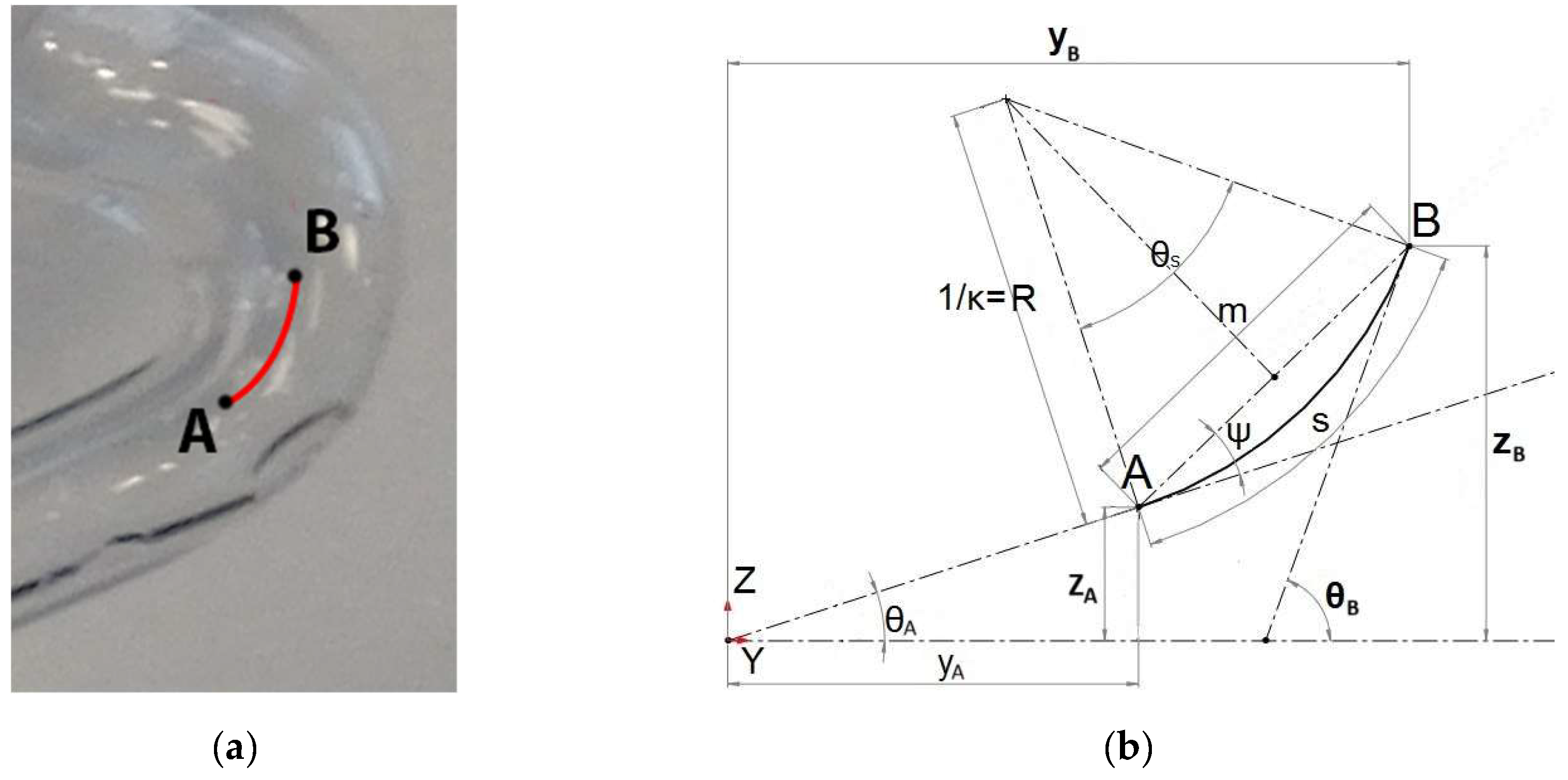
According to Figure 7(b), the angle, horizontal coordinate y, and vertical coordinate of point B are given by the following Equations:
The angle ψ is defined such that its sides are perpendicular to those of the angle θs/2, leading to:
For the angle θs, considering that the curvature κ equals 1/R, we have:
As for the length m, it is calculated as follows:
Substituting ψ, θs and m from Equations (4), (5) and (6) into Equations (1), (2) and (3), respectively, we derive the following expressions for the coordinates and angle of point B:
For straight pipe segments, the above Equations degenerate into the following:
Equations (10), (11) and (12) for straight pipe segments apply not only to the straight sections of the composite pipe of the burette but also to volumetric cylinders and conical flasks, whether wide-necked or not (Figures Figure 3 and Figure 4).
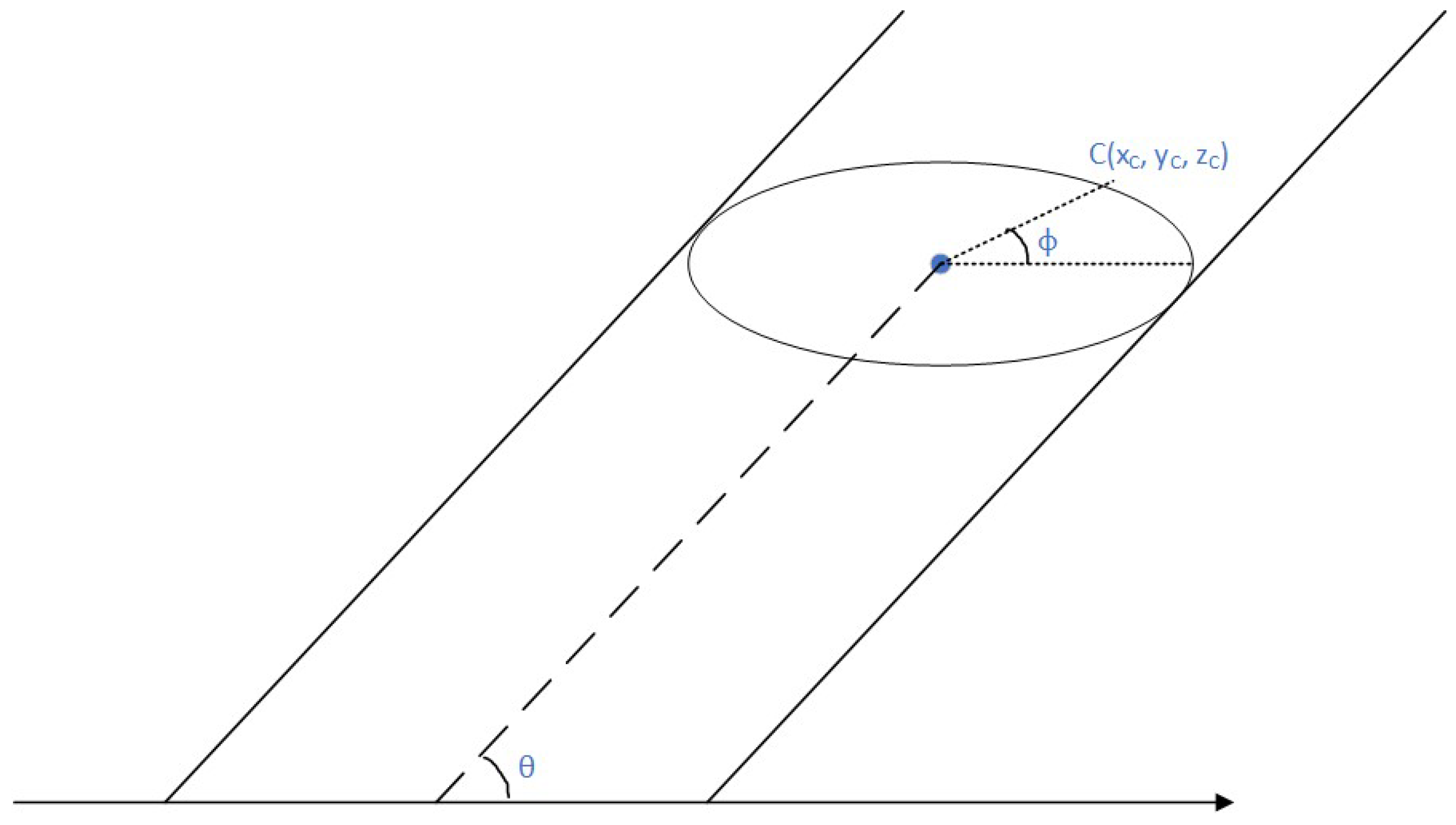
3.1.4. Geometric and Mathematical Description of the Coordinates of the Perimeter of a Pipe or Vessel with an Inclined Circular Cross-Section
Initially, we will describe the mathematical coordinates of a random point C on the liquid’s perimeter in a pipe with an inclined circular1 cross-section (Figure 8). Knowing the coordinates of the points on the circular perimeter, we can later in Unity draw a polygonal approximation of the latter. By successively drawing the perimeters corresponding to each point on the central line, we have the full liquid lateral surface inside the pipe.
Figure 8.
The circular cross-section of an inclined pipe with the horizontal level.
In order for the calculation to be done, the diagram in Figure 8 is deployed into the ones of Figure 9.
Figure 9.
(a) Cross-sectional view at a point on the central line with a horizontal orientation. (b) Central-line plane of a pipe segment.
Figure 9.
(a) Cross-sectional view at a point on the central line with a horizontal orientation. (b) Central-line plane of a pipe segment.
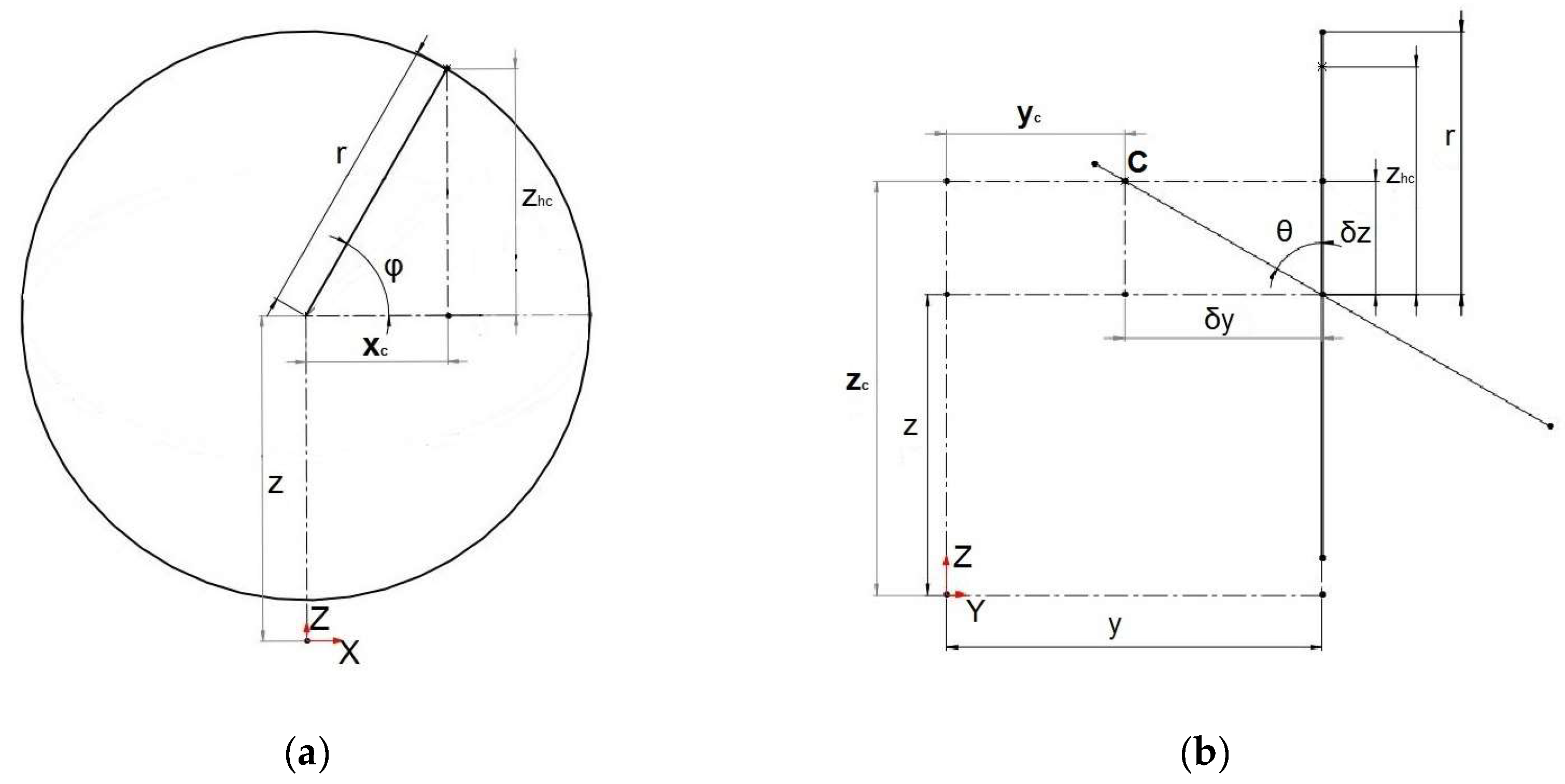
From Figure 9(a), we have:
Now, according to Figure 9(b), when the cross-section is inclined by angle θ, can be analyzed into dy and dz as follows:
Combining Equations (14) and (15) with the z-coordinate of the point on the central line of the cross-section, and Equations (14) and (16) with the y-coordinate of the same point on the central line of the cross-section, we derive the general Equations for the points of the circular perimeter in 3D space:
We remind that xc is already given in Equation (13).
3.2. Discretization of Pipes and Bottles’ Cross-Sections
In sections 3.1.3 and 3.1.4, we calculated the Equations for the co-ordinates of any point on a central line as well as the Equations for the co-ordinates of the respective points on the central line’s circular cross-section with the horizontal level. Having done so, we can dynamically create in Unity the meshes of the interior liquids of the various vessels of our simulation.
However, the circles upon which the liquid mesh creation is made cannot obviously be drawn as such. Instead, we approximate those with polygons through a process called discretization. The latter depends heavily on the number of vertices we decide our polygons to have (Figure 10).
Figure 10.
An example of 8-point discretization.
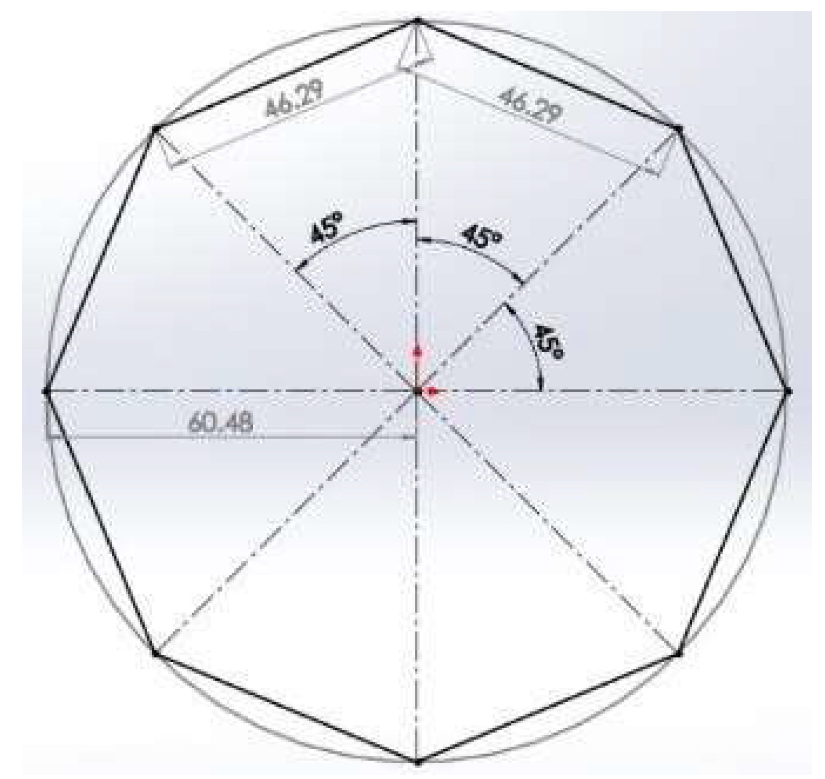
Figure 11 shows the notation for points in each cross-sectional circle.
Figure 11.
Discretization notation in cross-sectional circles.
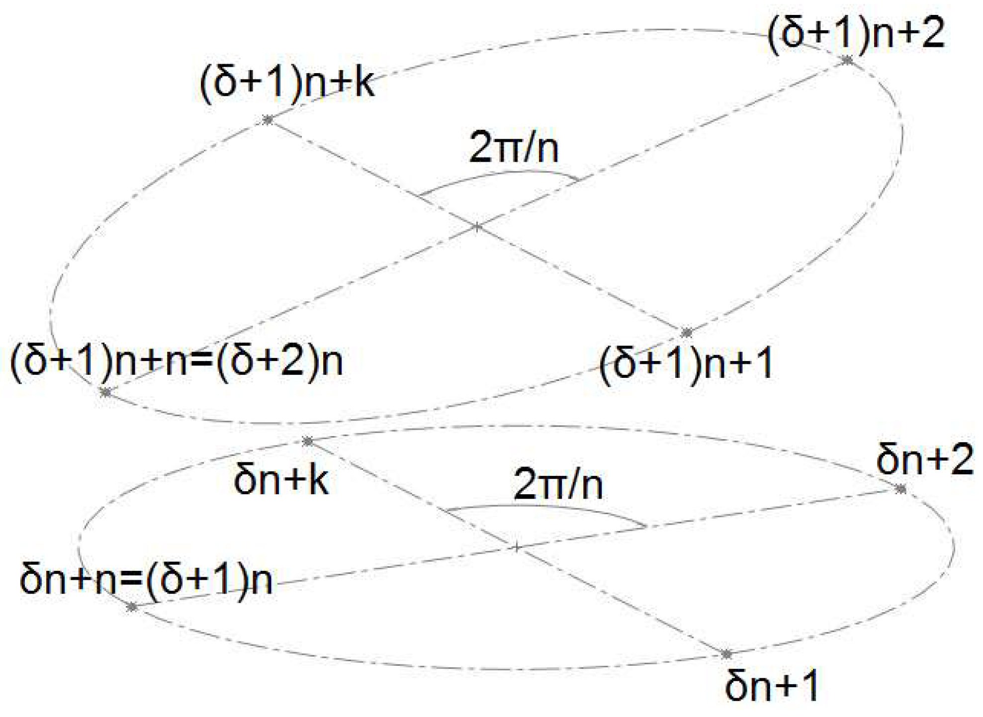
Specifically, in Figure 11, δ represents the cross-section number, ranging from 0 to the total number of cross-sections minus 1, while k denotes the sequential number of the point within each cross-section, ranging from 1 to the total number n of discretization intervals.
The number n, chosen by the developer of the simulation, applies to all cross-sections and determines the fidelity of the circle representation. In the example above, the value of n equals 4.
The coordinates of the aforementioned points will be calculated based on angular intervals of 2π/n at angles ϕk=k⋅2π/n. In this specific example, the angles are π/2, π, 3π/2 and 2π. For these angles, using the radius of the circle of the current cross-section, the inclination of the cross-section, the coordinates of the circle’s center (the central line point), and Equations (13), (17) and (18), the coordinates of each discretized point of the circle/cross-section are computed.
This method of notation—continuous sequential numbering of the discretized points of cross-sectional circles—was mandated by the way points are defined in Unity’s method for creating triangular finite surface elements. In this method, the sequential number of each point is declared in a one-dimensional array whose elements are the above 3D points (Vector3 variable type).
3.2.1. Definition of Triangular Surface Finite Elements Using Cross-Section Points
The following figures illustrate possible combinations of points forming surface finite triangles. Connections are chosen only between neighboring points within the same cross-section and points at adjacent angles between neighboring cross-sections, as shown in Figure 12.
Figure 12.
Connections Between Points for Optimal Resolution.
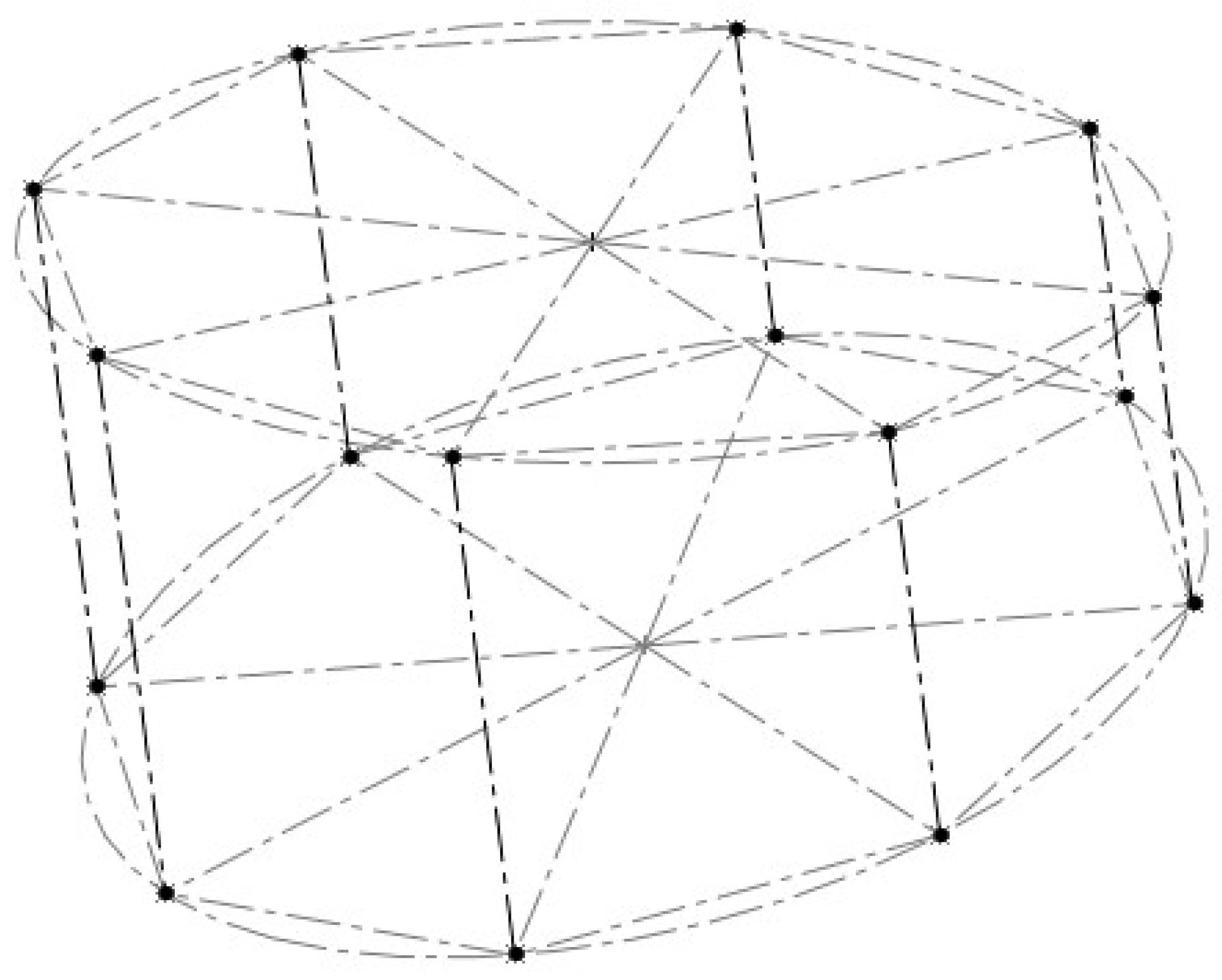
Each point on the last cross-section can participate in two to four triangular elements.
Each line connecting points of adjacent cross-sections at the same angle forms the edge of exactly two triangular elements. Consequently, the total number of triangular elements equals 2n.
Each such line can participate in three different triangular element combinations; that is, one edge of each triangle always starts in one cross-section and ends in the neighboring cross-section and at a neighboring angle:
- Triangles with one edge in the previous cross-section.
- Triangles with one edge in the last cross-section.
- Triangles with edges in different cross-sections.
Figure 13 illustrates the triangle combinations for each edge between cross-sections at the same angle.
Figure 13.
Triangle combinations for each edge between cross-sections at the same angle.
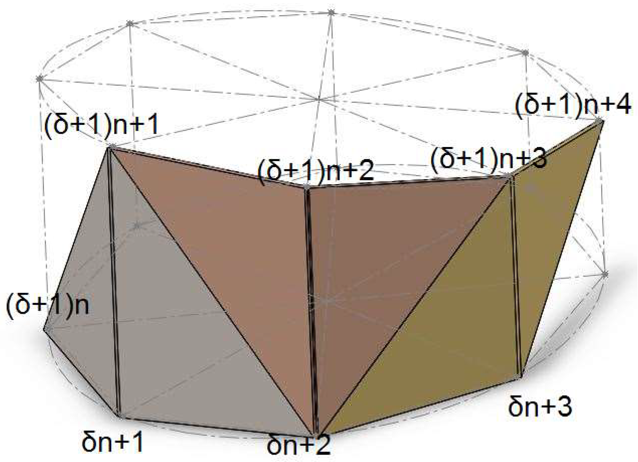
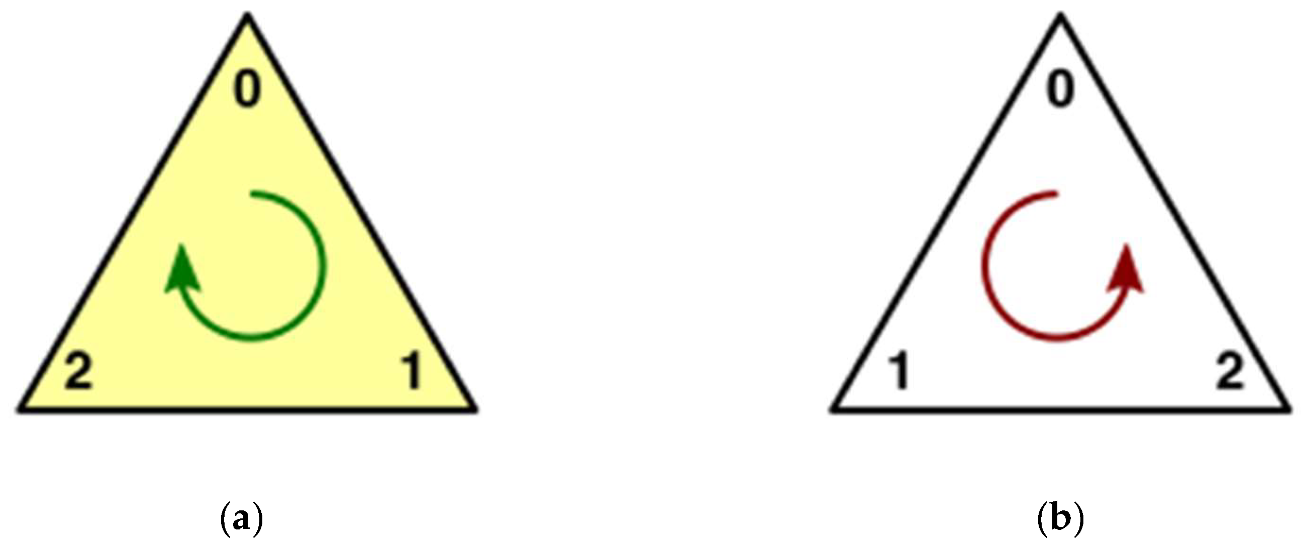
To ensure the visible side of the triangle (the outer surface in this application) appears in Unity, the order of point declaration for the triangle must follow a clockwise sequence (Figure 14(a)).
Figure 14.
Orders of point declaration for visible surface side: (a) Clockwise. (b) Counter-clockwise.
Figure 14.
Orders of point declaration for visible surface side: (a) Clockwise. (b) Counter-clockwise.
3.2.2. Mathematical Handling and Implementation Specifics of Triangles Between Cross-Sections
The diameters (d) of pipes/bottles (half of which is the radius r used in the circle coordinate Equations for inclined cross-sections) as well as the lengths (l) and the curvatures (κ) of the central lines are stored as data in a description matrix.
To account for potential tapering in the first section, the initial diameter must also be declared. For subsequent sections, since continuity between sections is assumed, the initial diameter of a section is determined by the final diameter of the previous section. For instance, for the second section, the initial diameter is d1 and the final diameter is d2.
Using the initial diameter of the composite pipe, the initial slope, and the starting coordinates of the central line, discretization points are generated in the initial cross-section to form the first triangular surface finite elements using the discretization points of the initial cross-section (excluding the start point).
The surface between two points on the central line is created through the following steps:
- Assuming a sufficiently small step length for the central line and incrementally increasing the current length in a loop.
- Calculating the coordinates of the central line point corresponding to the current length at each iteration.
- Based on the above coordinates, iteratively calculating the discretization points of the cross-section’s perimeter using angular intervals (as determined by the chosen resolution). These points are recorded sequentially in a one-dimensional array.
- Using the discretization points of the previous and current cross-sections, triangular surface finite elements are created by recording the sequential numbers of each point in the previous array. Each set of three points, in order, forms a triangular element. The two arrays are assigned as corresponding vertex and edge attributes in a mesh structure.
To minimize iterations and algorithm execution time (thereby reducing time between iterations, improving dynamic simulation of level variations, and increasing surface accuracy), the grouping of vertices for triangle creation is further analyzed. That is, the existence of a possible pattern for the set of each cross-section is investigated so that the implementation can be included in the existing point/peak generation loop.
For each cross-Section , starting from the first defined point , the following two triangular finite elements can be declared using points from the previous cross-section:
and
For the next point , combinations with points incrementally higher than those in the previous sets are tested:
and
Following this approach, triangular finite elements are defined sequentially for the last point in the current cross-section:
and
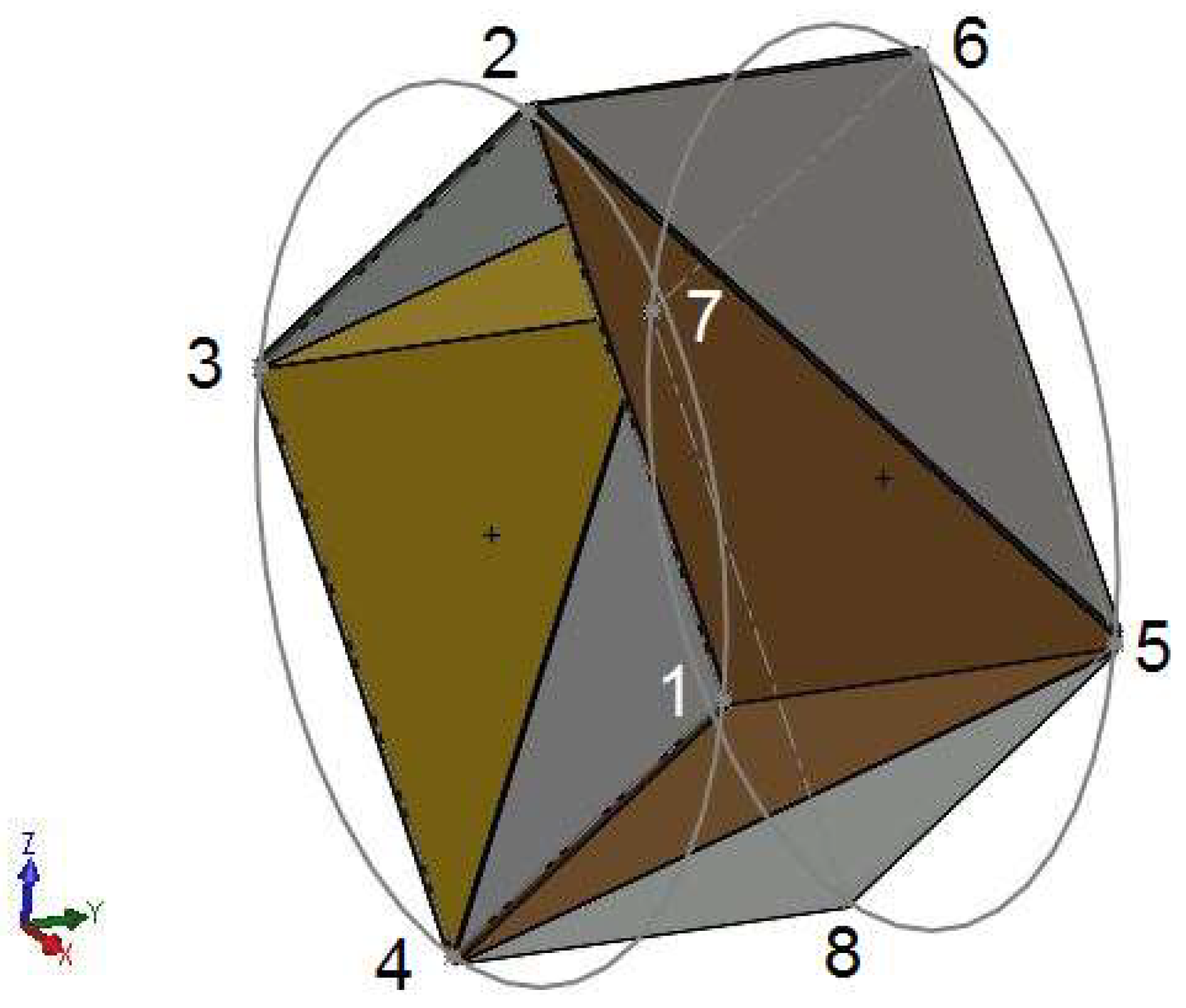
Figure 15 illustrates a graphical depiction of the sequence for recording/representing the triangular finite elements for each point of a cross-section with 4 discretization points.
Figure 15.
Creation of triangles from the first point of the new cross-section (point 5).
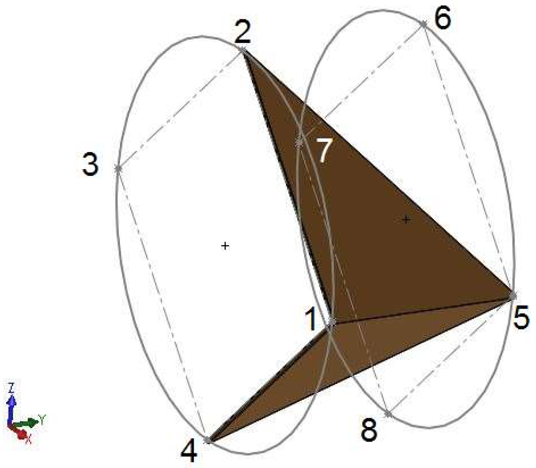
In Figure 15, the triangles that can be defined after creating the first point of the new cross-section (point 5) are shown. Thereby the two created triangles for point 5 are:
and
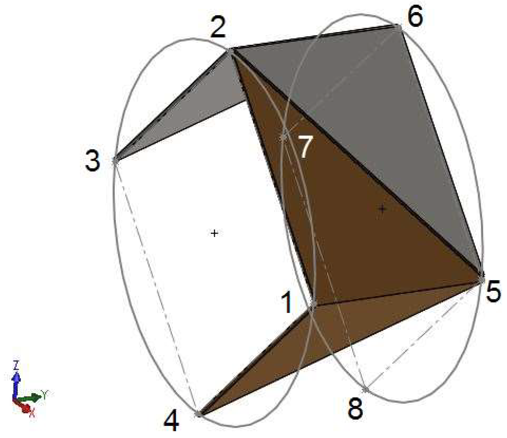
Next, the triangles for the remaining three points of the cross-section are created (at this point, in addition to the points from the previous cross-section, the neighboring points of the new cross-section that have already been created are available).
Thus, the triangles for point 6 (Figure 16) are:
and
Figure 16.
Creation of triangles from the second point of the new cross-section (point 6).
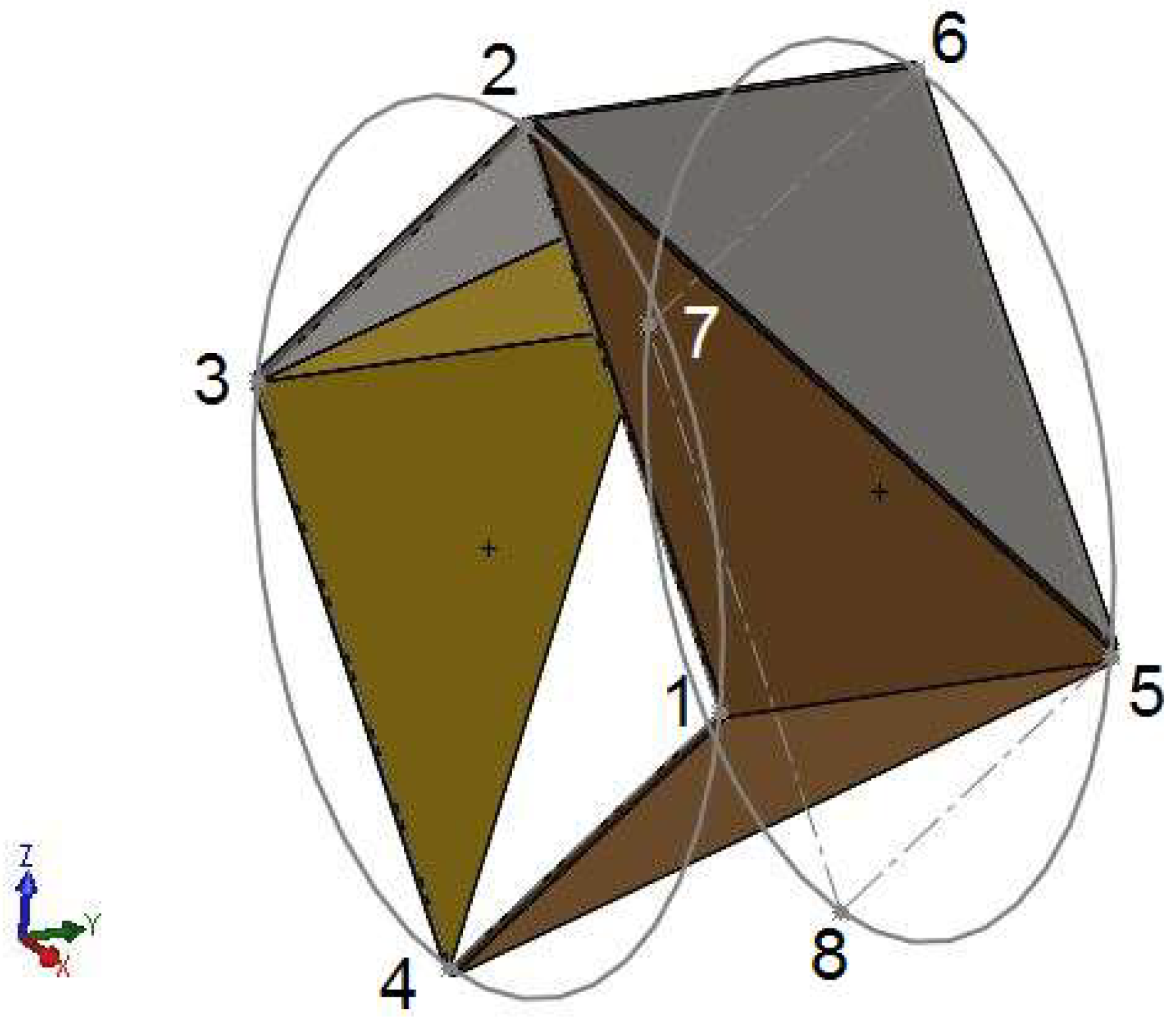
Next come the triangles for point 7 (Figure 17) which are:
and
Figure 17.
Creation of triangles from the penultimate point of the cross-section (point 7).
Finally, the triangles for point 8, which is the last point of the cross-section (Figure 18) are:
and
Figure 18.
Creation of triangles from the last point of the cross-section (point 8).
In total, we have the following pairs of triangles for each of the points 5, 6, 7 and 8:
and
and
and
and
It is easily observed that for a point with a total serial number and being the number of discretization points in each cross-section, a numerical pattern is followed for the point’s two triangles:
and
For the next point , the numbers in the above triplets forming the finite triangular elements are increased by 1 (that is, the next point from the corresponding triplets of the previous point is recorded):
and
This pattern can be directly utilized in implementation to generate the finite surfaces simultaneously, without requiring a new loop, during the creation of discretization points for each cross-section.
3.3. Simulation of Dynamic Flow and Liquid Level Variation in Bottles and Tubes
As mentioned in section 3.1, the developed methodology for modeling the surface of tubes and liquids aims to define the surface as a function of a single variable, that of the current local length of the bottle or tube segment. By knowing the current local length—representing the liquid level for bottles or the volume in general for the container (bottle or tube)—and the characteristic data of the container (from the corresponding registry), the current diameter and local slope of the container at every point along its centerline are calculated accordingly. This approach enables the generation of the corresponding surface from the base to the current length of the container.
The goal of this modeling effort has been, from the outset, the dynamic simulation of liquid level variation during filling or removal from the container. The developed methodology successfully separates the implementation of surface creation from the mathematical modeling of the one-dimensional dynamic liquid flow (which dynamically provides the current liquid volume in each container).
The remaining task is to mathematically calculate the local liquid level (the current length) in each circular cross-section container, assuming that the simplifying assumptions are outlined in section 3.1.2 are adhered to. The resulting function for calculating the local current length and slope is used as input to the implementation described in section 3.1 to design the corresponding surface as its outcome.
The mathematical modeling of liquid flow is achieved using fluid mechanics Equations. Subsequently, a mathematical approach is presented for modeling the filling of a bottle under a known liquid volume flow rate.
In cases where the filling occurs with a known liquid volume flow rate over time, the bottle is filled by transferring liquid via free flow (without losses and at atmospheric pressure) from a different container.
To calculate the instantaneous liquid volume flow rate into the target bottle, it suffices to know the outflow velocity, the cross-sectional area of the outflow opening of the supply container, and the proportion of volumetric outflow directed into the target bottle. The instantaneous flow rate is given as the product of these three factors, which can be determined by solving a system of fluid mechanics Equations for the flow within the supply container.
3.3.1. Geometric and Mathematical Description of Bottle Levels with Respect to a Known Liquid Flow Rate
Given a liquid flow rate—either constant or expressed as a time-dependent function—and knowing the time step of each iteration of the simulation loop (handled by a C# Unity function), the additional volume added to the tube between the previous and current iterations can be calculated. In this sense, the volume is treated as a known quantity.
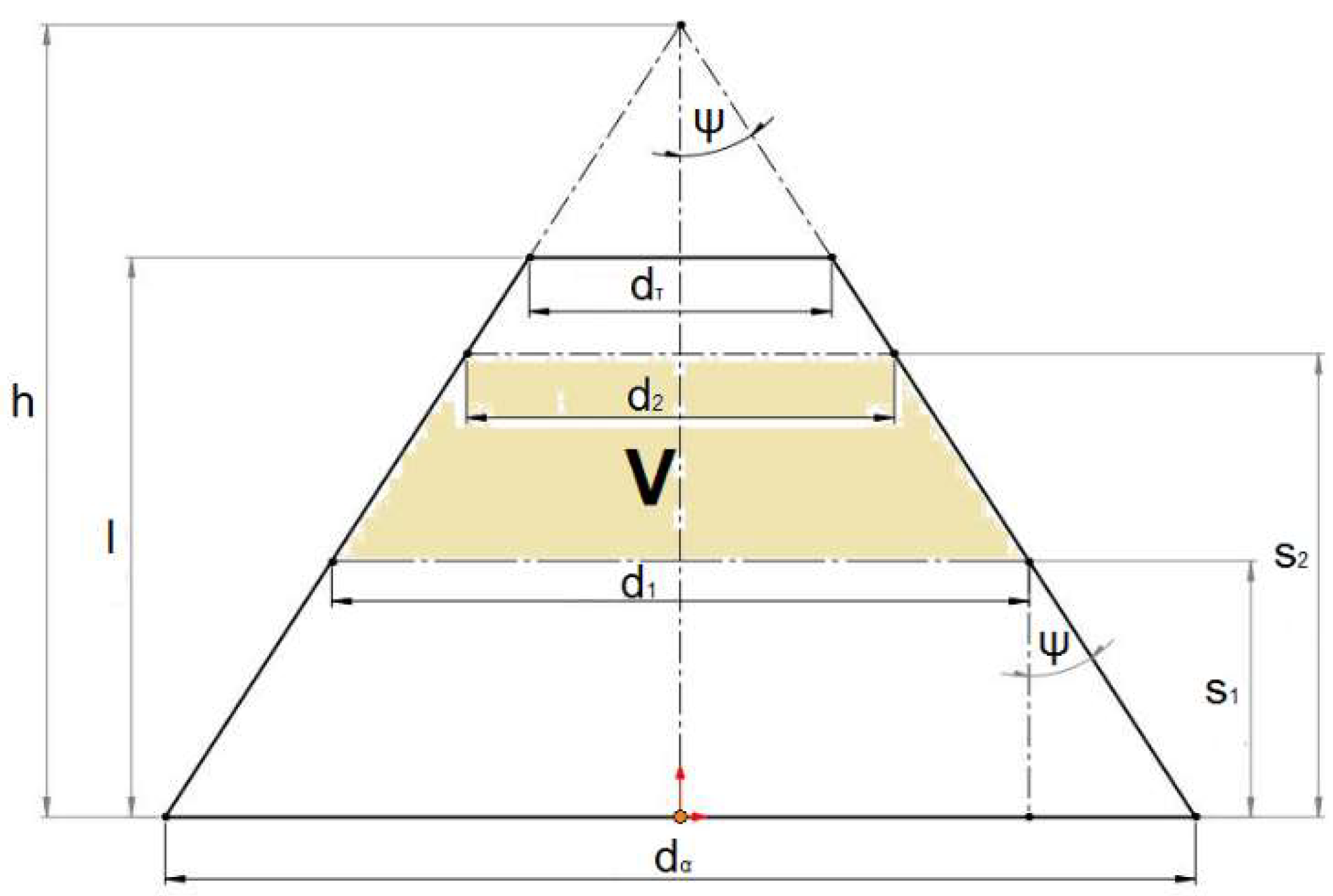
Figure 19 shows a schematic representation of a tube with an increasing diameter cross-section.
Figure 19.
Schematic Representation of Liquid Volume in a Diverging Frustum Cone as a Function of Its Level.
Figure 19.
Schematic Representation of Liquid Volume in a Diverging Frustum Cone as a Function of Its Level.
The volume V between two levels, s1 and s2, in Figure 19 is given by:
To relate parameter H with the levels and diameters, the tangent of angle ψ is used:
The linear function of diameter with respect to the level/point on the central axis of the tube is expressed as:
where the parameter equals the tangent of the cone angle :
In Equation (19), we substitute H with its value from Equation (20); we then substitute d1 and d2 with their values from Equation (21) for s being s1 and s2, respectively; and finally, we rearrange all terms to one side of the Equation, simplifying into terms of s2 (the level of interest).
The resulting Equation becomes:
Equation (23) is a complete cubic polynomial of the form:
The discriminant Δ is calculated as:
Substituting the coefficients, the discriminant becomes:
Since Δ is always negative, the Equation has one real solution and two conjugate complex roots. This result is desirable because, in other cases, there could be either three distinct real roots or one double real root and one single real root. The real root provides the exact analytical expression for the new liquid level based on the given data and the previous known level.
The general solution for Equation (24) is:
Substituting the coefficients from Equation (23), the real solution simplifies to:
Verification of this solution by substitution into Equation (23) shows the left-hand side becomes zero, confirming its correctness. Simplifying by cubing both sides and rearranging terms verifies equivalence to Equation (23).
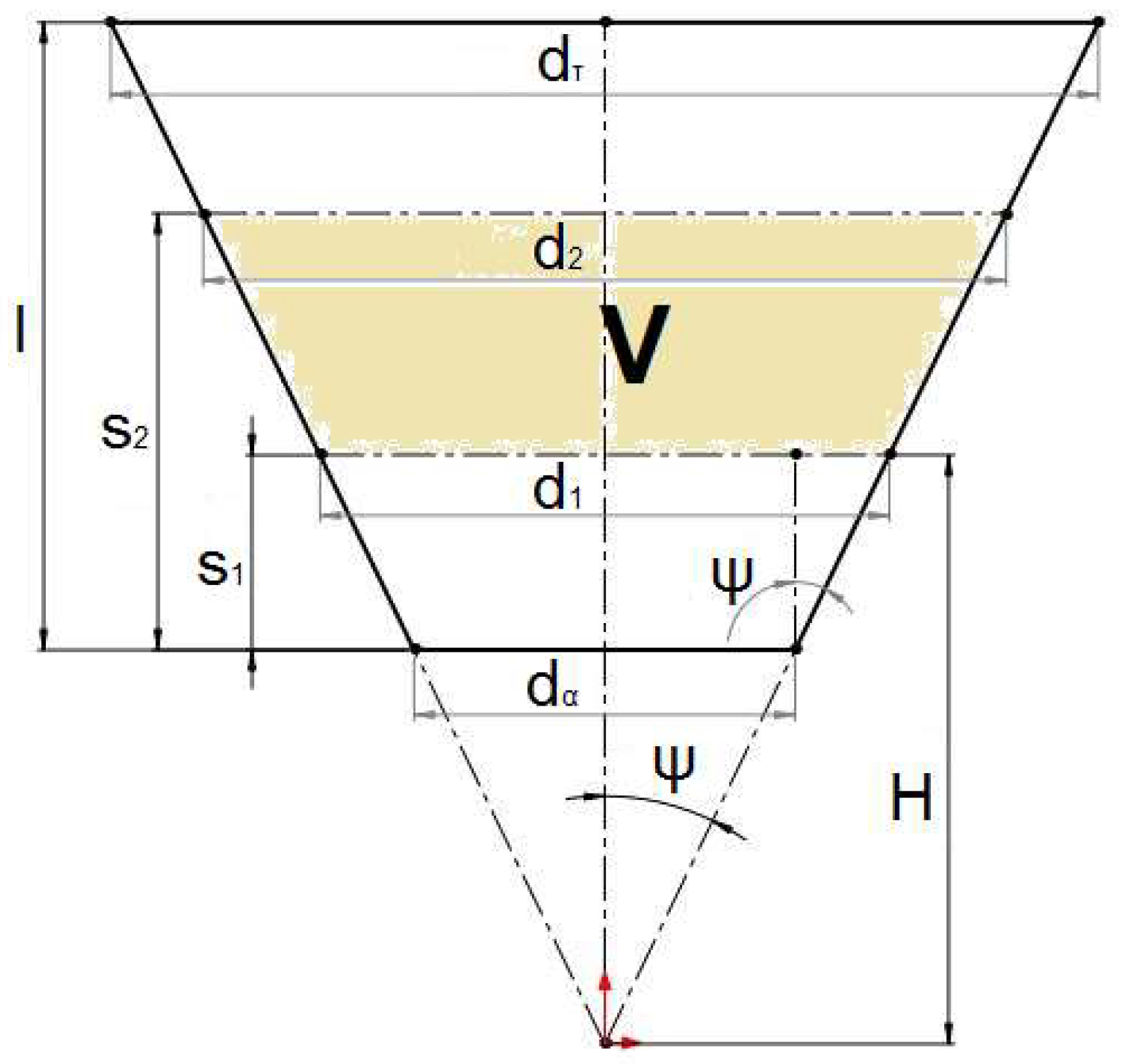
We will now consider the case of the truncated conical tube of decreasing diameter, according to the schematic representation of Figure 20.
Figure 20.
Schematic Representation of Liquid Volume in a Converging Frustum Cone as a Func-tion of its Level.
Figure 20.
Schematic Representation of Liquid Volume in a Converging Frustum Cone as a Func-tion of its Level.
The liquid volume V in Figure 20 is given by:
Using the tangent of angle ψ to relate h to the other parameters, we get:
The same process applied to Equation (28) results in a cubic polynomial identical to Equation (23). Hence, its solution is also identical to Equation (27).
For completeness, the case of a straight tube with constant cross-sectional diameter is included. For this case, therefore, we have:
3.3.2. Key Points and Implementation Examples for Bottle Filling in Unity
The modeling and implementation of surface creation accept the following as input parameters for the initial cross-section characteristics:
- coordinates of the central line point of the initial cross-section
- slope of the initial cross-section
- diameter of the initial cross-section
In the implementation, it is necessary to retrieve the time interval Δt that has elapsed since the previous iteration of the execution loop in the corresponding Unity C# script.
The implementation requires tracking and monitoring of the following variables:
- The current volume V of liquid in the bottle,
- The cumulative volume Vtot,i that each segment of the bottle can contain.
This information is critical to determine the segment of the bottle where the liquid level will rise after adding the new volume to the existing volume of liquid. Specifically, if the flow rate is sufficiently high (or the segment volume is sufficiently small) so that within the time interval between two loop iterations the liquid level can move through one or more segments, the surface can be rendered for all such segments up to the level of the current segment.
At the beginning of the implementation code (during the initialization function) and before the execution loop starts, the cumulative volumes stored from the bottom of the bottle to each segment Vtot,i are calculated and recorded.
The volume of a frustum of a cone with da and dτ being its bases and l its height (Figure 19) is given by the formula:
If, in Equation (32), dα and dτ are replaced by d (for a bottle segment with a constant cross-sectional diameter) and the length l is replaced by s2−s1, then the equation becomes identical to Equation (30).
Thus, Equation (32) can be used to calculate the individual volumes of all types of bottle segments examined in this study (constant-diameter and linearly varying diameter shapes).
We will now express the volume of a curved pipe section as a function of its length
We know from calculus [10] that the volume V of a solid of revolution, where the cross-sectional area is bounded by the functions R(x)=y1 and r(x)=y2, is given for the segment of the solid between heights α and β by the following integral:
In our case, we are interested in the volume of liquid within a segment of circular cross-section, as illustrated in Figure 21.
Figure 21.
Liquid volume within a segment of circular cross-section.
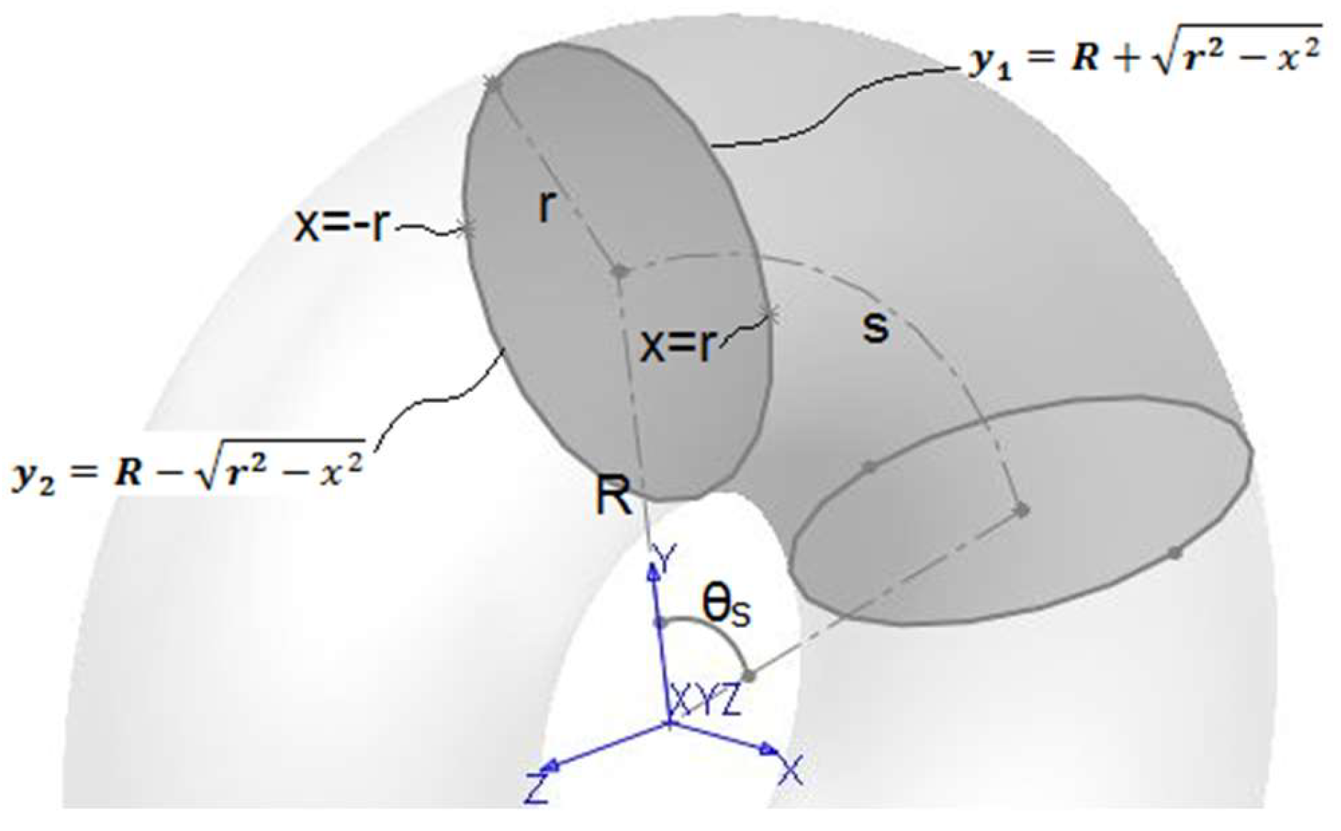
The upper semicircle in the said figure is expressed as:
while the lower semicircle is expressed as:
The resulting volume is:
For rotation through an angle θs, the volume Vs is expressed as:
By substituting s=θsRs, we get:
If we further replace s with s2−s1 and r with d/2, the equations remain consistent with Equations (30) and (32), which also hold for cylindrical volumes.
Before the execution loop begins, the points of the pipe’s initial cross-section are created, and if an initial liquid level exists, the points of the cross-section at the initial liquid level and the surface between them are also created. Finally, the initial volume is calculated (this functionality has been implemented for an initial level in the first segment). During the execution loop, based on the given liquid flow rate, the new volume of liquid to be added to the pipe for each time interval between iterations is calculated as ΔV=Q⋅Δt. The new total current volume is then compared with the cumulative volumes up to each segment to determine in which segment the new liquid level will be located:
Two cases are distinguished: if the new volume remains in the same segment as the previous one, the new liquid level is calculated using V=Vloc=ΔV and either Equation (27) or (31), depending on whether the segment’s diameter is variable or constant. Otherwise, if the new volume spans multiple segments, and if the new volume exceeds the total volume of the composite bottle, the entire bottle surface is rendered, and the loop execution is terminated. If not, the surfaces up to the previous segment are rendered, and the local volume for the current segment is calculated as:
This value is then substituted back into either Equation (27) or Equation (31), depending on whether the segment’s diameter is variable or constant (where s1, the initial level, is replaced with zero).
4. Results
In this section, we present the implementation results of our techniques in Unity. First, we illustrate various shapes of liquids implemented under our liquid simulation technique and the discretization process for their circular cross-sections. Afterwards, we show the outcomes of our dynamical flow simulation technique though consequent screenshots from the filling of vessels of various forms.
Unity requires the definition of unit normal vectors at each point of a mesh’s surface (through the mesh.normals property of the mesh structure). These vectors are used to determine shading and reflected lighting on the surfaces, providing the illusion of curvature even on individual triangles. In this implementation and the examples provided, Unity’s built-in method mesh.RecalculateNormals() was utilized. This method calculates the appropriate unit normal vectors for the created mesh.
The Unity implementation described here is based on the implementations available on the Flick website [11].
Figure 22.
Creation of a volumetric cylinder’s mesh with 4-point discretization.
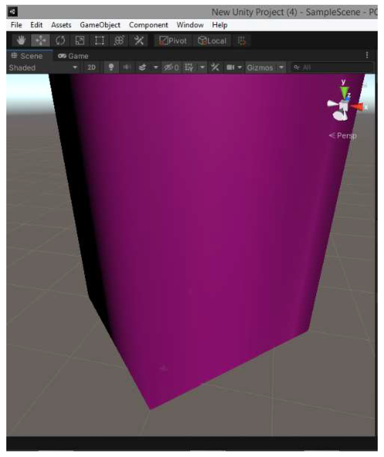
Figure 23.
Creation of a volumetric cylinder’s mesh with 10-point discretization.
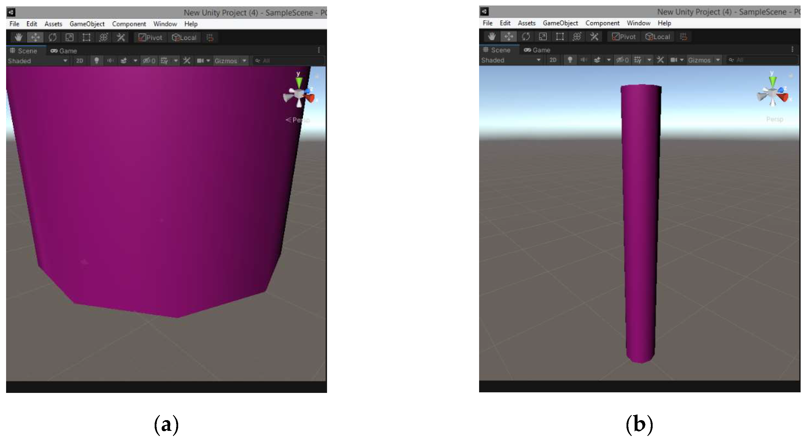
Figure 24.
Creation of burette’s mesh.
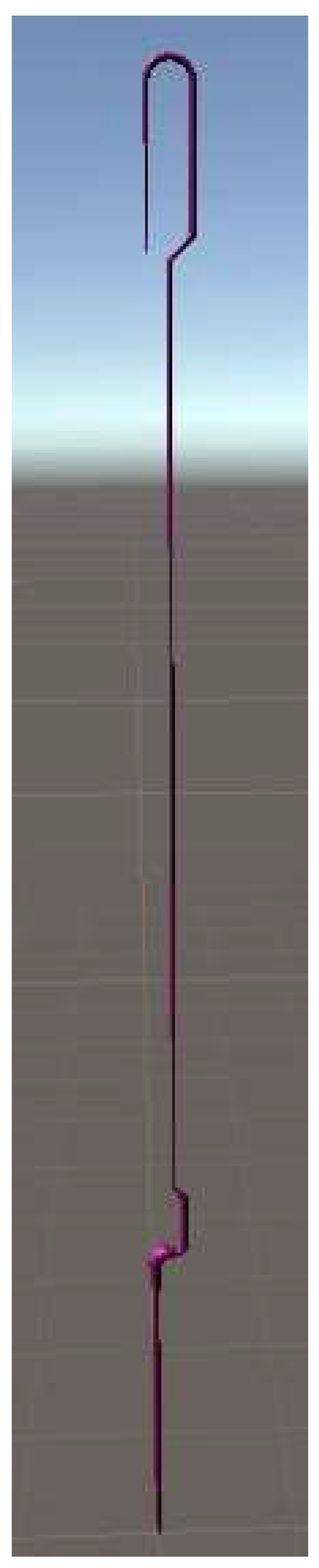
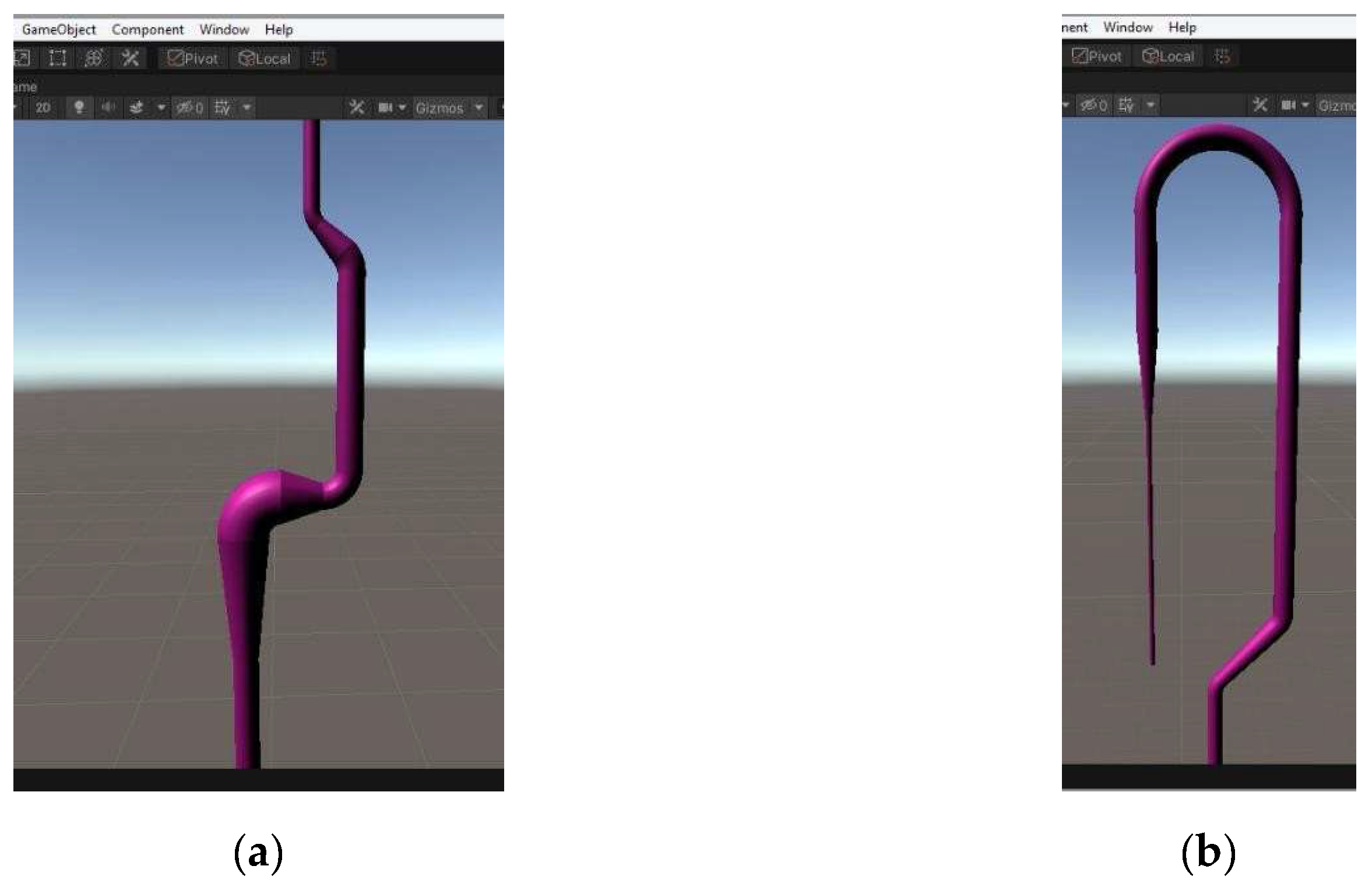
Figure 25.
Detailed view of various parts of burette’s mesh.
We now present video screenshots of the implementation of the liquid filling for three kinds of vessels, conical flask, wide-neck conical flask and volumetric tube, already discussed in previous sections, with a volume flow rate equal to 10000 mm3/sec.
Figure 26.
Simulation snapshots of a 200ml conical bottle filling simulation in Unity.
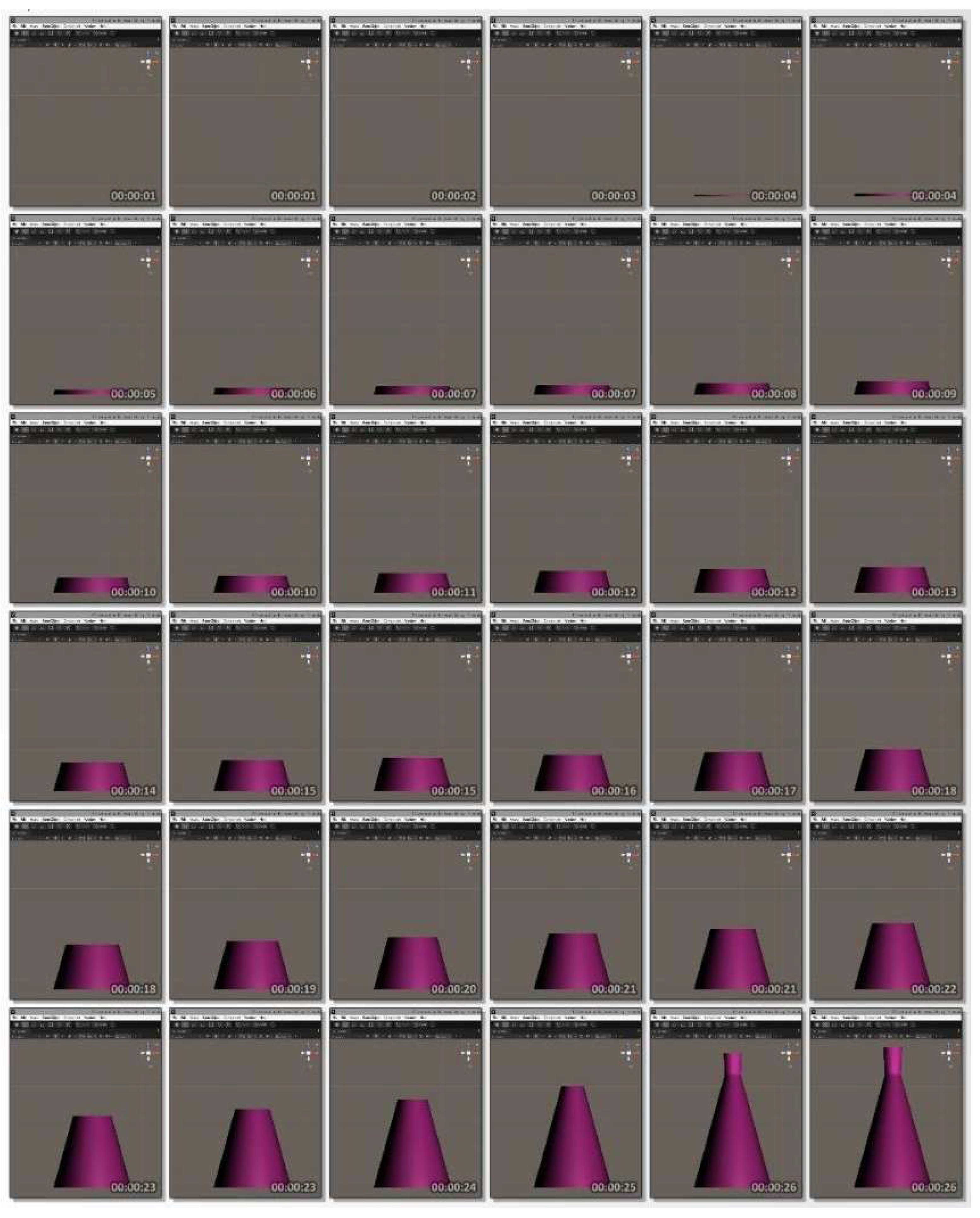
Figure 27.
Simulation snapshots of a 100ml volumetric tube filling simulation in Unity.
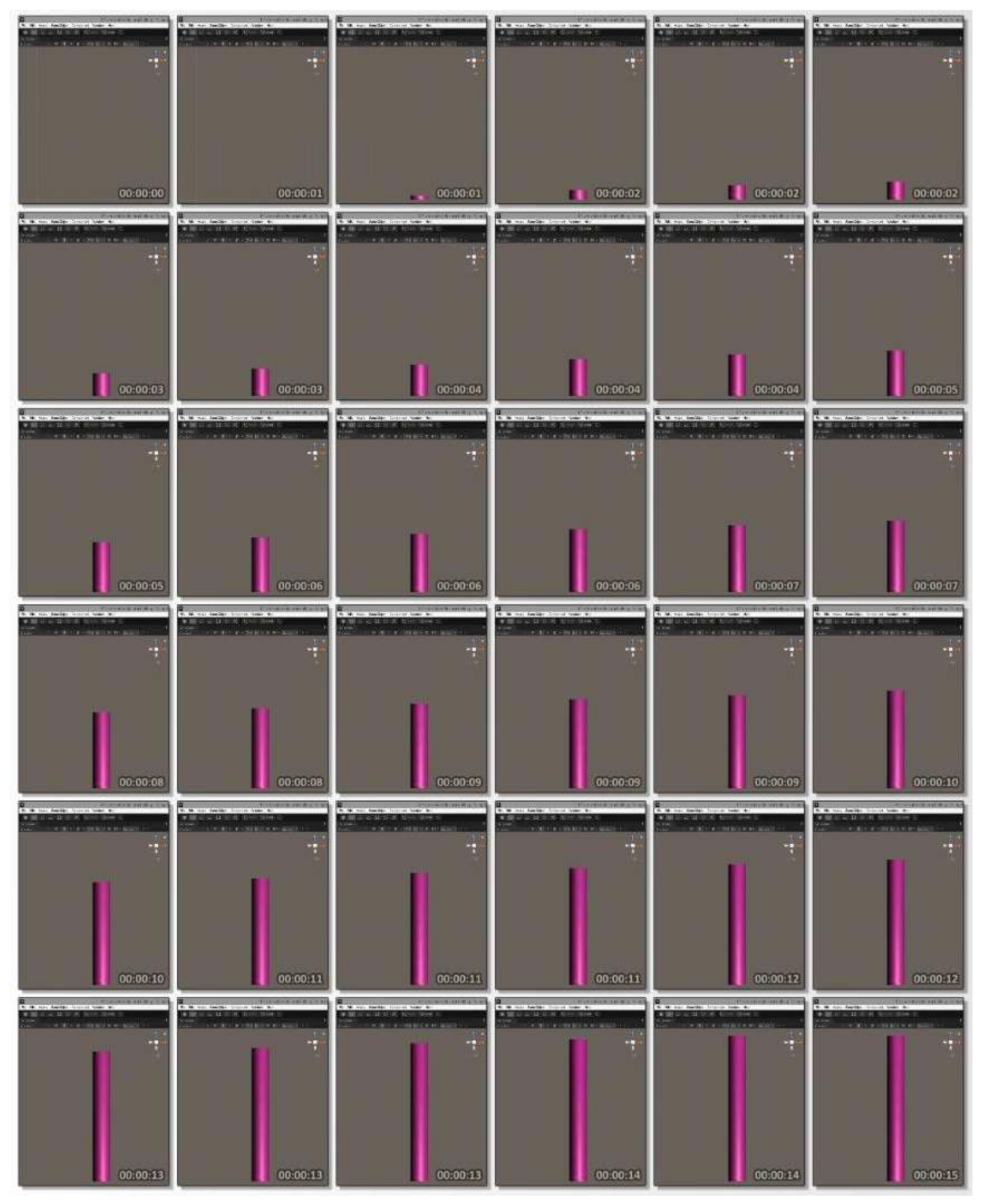
Figure 28.
Simulation snapshots of a 250ml wide-necked conical bottle filling simulation in Unity.
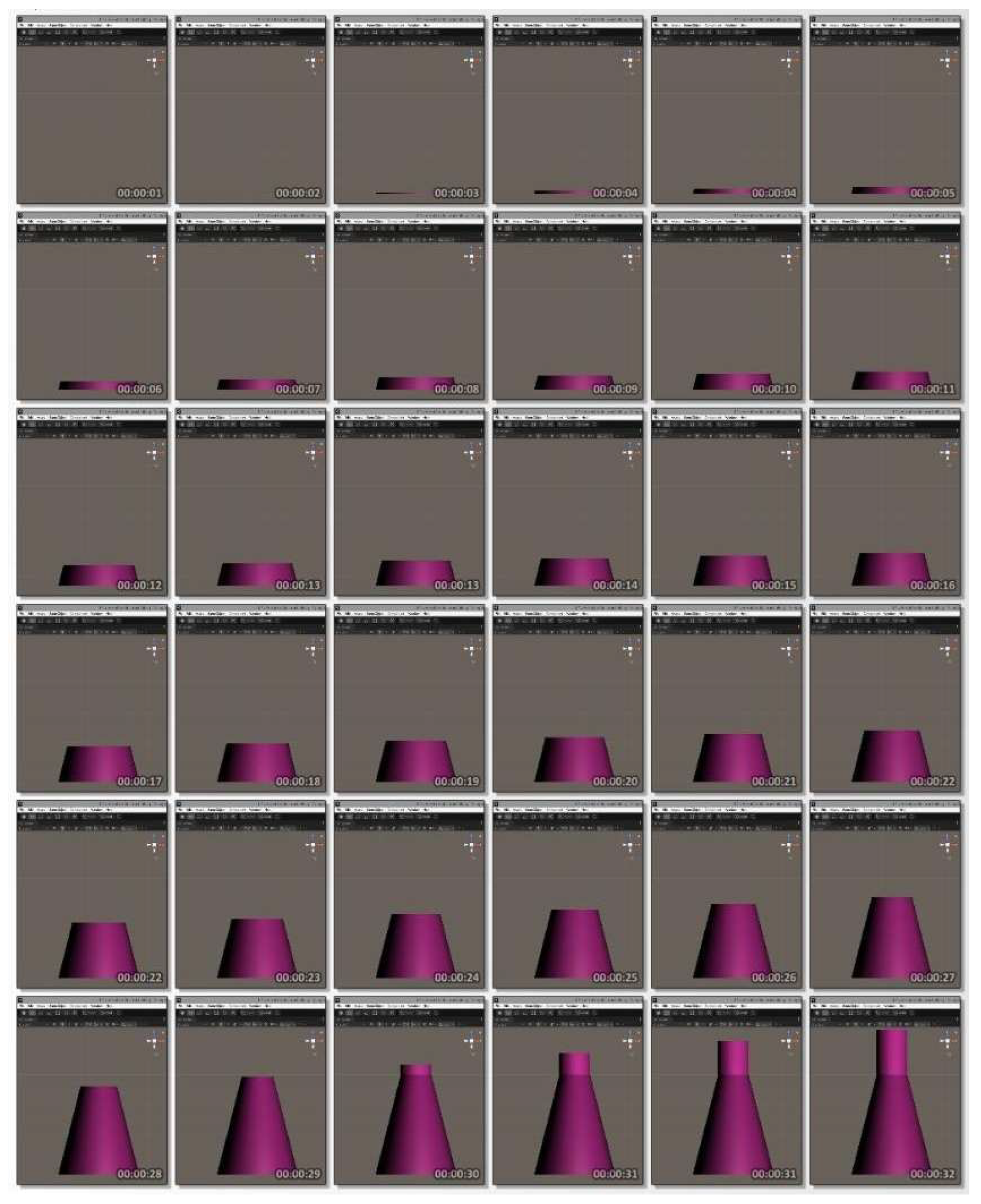
Table 1 shows the calculations of the volumes of the bottles and the time they are expected to be fully filled, according to the assumed volume supply.

Table 1.
Calculated volumes and filling times of liquid vessels.
| Vessel Type | Diameter dα (mm) | Diameter dτ (mm) | Length l (mm) | Volume V (mm3) | Flow rate Q (mm3/sec) | Filling time t (sec) |
| Conical Bottle 200ml | 78 | 16 | 112 | 22491.7805 | 10000 | 22.24917805 |
| 16 | 19 | 27 | 6510.165376 | 10000 | 0.651016538 | |
| Total | 22.90019459 | |||||
| Volumetric Tube 100ml | 27.5 | 27.5 | 225 | 133640.4062 | 10000 | 13.36404062 |
| Wide-Necked Conical Tube 250ml | 82 | 31 | 100 | 257742.2339 | 10000 | 26.77422339 |
| 31 | 31 | 45 | 33964.54358 | 10000 | 3.396454358 | |
| Total | 30.17067775 | |||||
Hence, we observe the following:
- The conical flask is filled from the 3rd to the 26th second, a duration of 23 seconds, which aligns approximately with the calculation in Table 1.
- The graduated cylinder is filled from the 1st to the 14th second, a duration of 13 seconds, which also matches the calculation in Table 1.
- The wide-necked conical flask is filled from the 2nd to the 32nd second, a duration of 30 seconds, again consistent with the calculation in Table 1.
This confirms the accuracy of the simulation and modeling of the filling process achieved by this implementation.
Finally, the result of simulating the filling process of the conical flask, along with the time intervals in seconds for a flow rate of 1,000,000 mm³/sec (1 liter/sec), is presented in Figure 29.
Figure 29.
Simulation result of filling a conical flask at a flow rate of 10⁶ mm³/sec.
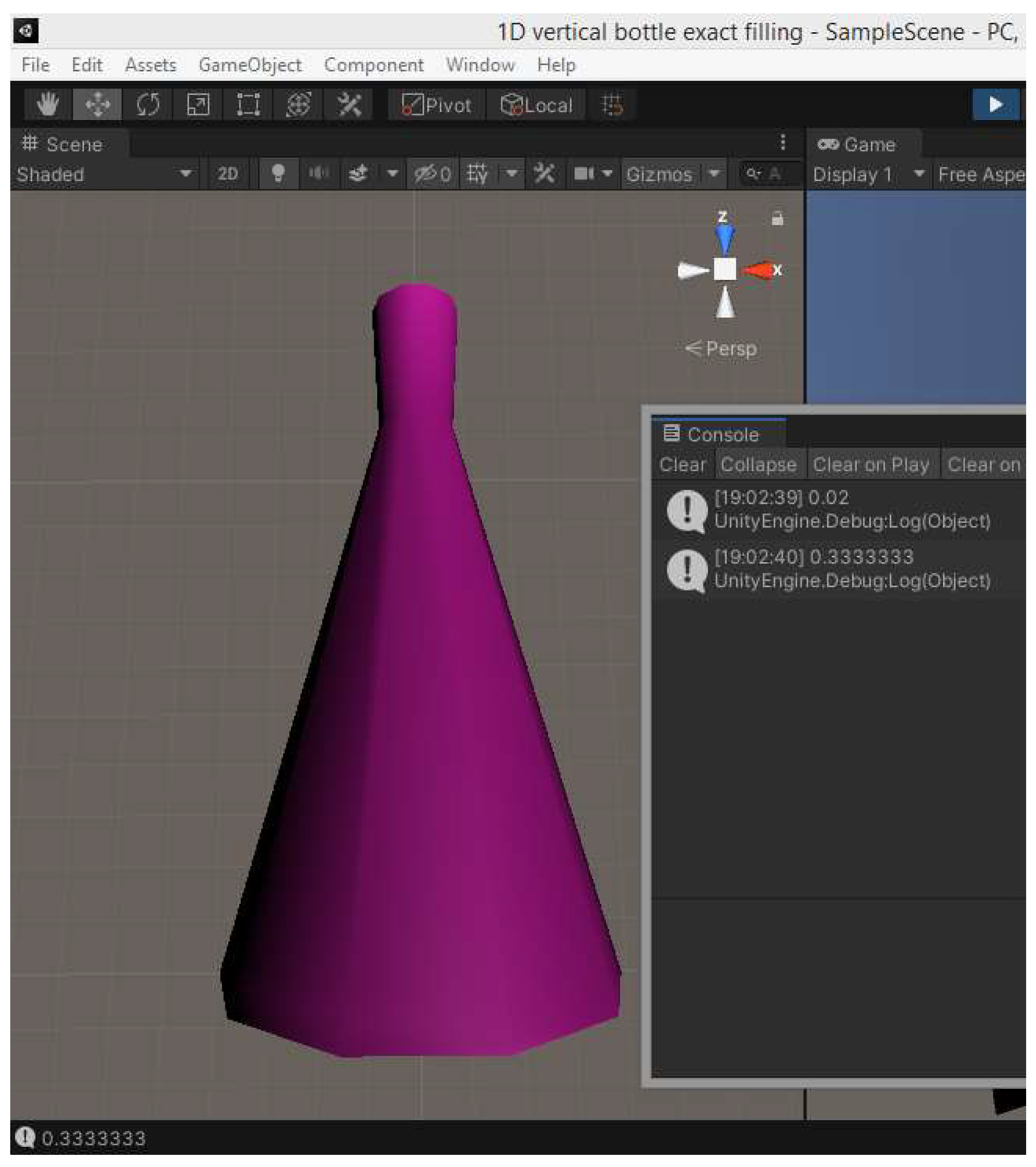
At this flow rate, it takes approximately 0.22 seconds to fill the first segment. It is observed that during the first iteration, the time duration is 0.02 seconds, and 20,000 mm³ of the approximately 222,500 mm³ of the first segment and the total of approximately 229,000 mm³ of the flask are filled. In the second iteration, after 0.33 seconds, 330,000 mm³ could potentially be filled, but only 209,000 mm³ remain to fill the entire flask. The implementation determines the segment in which the liquid level should now be located based on the new total liquid volume and simultaneously fills each segment that is exceeded by the new volume. Once it determines that the total flask volume has been exceeded, the execution loop terminates.
It is noted that with the current implementation, the average time duration between iterations of the execution and rendering loop ranges between 0.017 and 0.036 seconds, using an NVIDIA GeForce GT 740M graphics card and an i5-4200 CPU at 1.60Ghz, with 8GB RAM.
Additionally, the image processing frequency of the human eye-brain combination ranges between 30 and 60 frames per second [12], indicating that the minimum time interval perceptible by the brain between two images is between 0.0166 and 0.0333 seconds. Thus, in terms of the sense of continuity and realism of motion, the implementation is considered satisfactory.
5. Discussions
In this study, given the complexity and extensive workload required to complete the specific experimental process, it was concluded that standardizing the process of recording and analyzing objects, their interactions, and the sequence of these interactions between entities and the user-learner is essential. This analysis can be represented in a modified state diagram, where the required interactions between entities and the user are mapped.
With the above recording of objects and actions, the simulation designer and programmer can design objects and their actions with the necessary functional detail (in terms of the required number of objects for each assembly and their necessary functions) without designing individual objects that serve no purpose.
The ease of design with parametric design software and the conversion of objects into graphical files for use in Unity was demonstrated. Subsequently, realism was approached by creating a sense of liquid level movement during the filling of flasks and tubes.
The approach focused on bottles and tubes with circular cross-sections of constant or linearly varying diameter (conical flasks and tubes). The flow in curved tubes was also examined. The flasks studied were vertical, while the central lines of the tubes lay on a common plane.
The filling of flasks was simulated using precise expressions that describe it. Potential extensions could include:
- Implementing the simulation of flask emptying (the same expressions apply, but adjustments would be needed in handling, such as the surface mesh).
- Accurate modeling of filling and emptying flasks with varying diameters using other analytical functions of the pipe length, apart from the linear function.
The filling of tubes was modeled using simple steady-flow expressions that approximate the actual liquid behavior, especially when applied to the automatic burette, where liquid-air interaction (compressible/elastic medium) is also present. Despite this, significant realism was achieved in real-time.
The dynamic liquid flow in a tube offers many improvements and extensions, such as:
- Combining energy conservation equations, mass conservation, loss calculations, and the ideal gas law for air to derive an analytical solution for the liquid-air interface velocity.
- Extending the modeling equations to describe the same types of tubes in space rather than only in the plane.
- Utilizing the PISO algorithm with exact dynamic flow equations for real-time implementation.
- Further extending the tube shapes to other analytical functions of circular cross-section diameter beyond the linearly varying and constant ones.
From an implementation perspective in C#, Unity’s blog mentions that lists are the ideal dynamic data structure for reducing computational time and space. In this study, a dynamic array was used. However, regardless of the use of dynamic data structures, current implementations can be significantly improved, as many iterative structures and control structures of procedural programming are used, and no particular emphasis was placed on optimizing the simulation implementations.
It would be possible to implement functionality that, based on the tube characteristics provided as input, the algorithm calculates local loss coefficients independently according to relevant rules.
Finally, a significant enhancement to the capabilities of a dynamic liquid flow/level simulation application would involve separating into distinct functions with the ability to collaborate:
- Modeling the coordinates and slopes of each point of a tube’s central line.
- Identifying the type of tube through analytical expressions for cross-section diameter variation and generating surface point meshes.
- Creating finite triangles and representing the surface using them.
Funding
This research received no external funding.
Acknowledgments
The text of this paper contains context-setting information and generic descriptions which also appear in some other work (properly referenced) by the same co-authors. The paper contains substantial new information (sections 1.2, 3, 4 and 5) which constitute new work.
Conflicts of Interest
The authors declare no conflict of interest.
| 1 | We remind that according to our assumption, the cross-section of a pipe with the horizontal level is always circular. |
References
- de Levie, R. A General Simulator for Acid-Base Titrations. J. Chem. Educ. 1999, 76, 987. [CrossRef]
- Zafeiropoulos, V.; Kalles, D. Quantitative Liquid Simulation in an Interactive 3D Virtual Laboratory. In Proceedings of the Proceedings of the 22Nd Pan-Hellenic Conference on Informatics; ACM: Athens, Greece, November 2018; pp. 219–224.
- Foster, N.; Metaxas, D. Realistic Animation of Liquids. Graphical Models and Image Processing 1996, 58, 471–483. [CrossRef]
- Harlow, F.H.; Welch, J.E. Numerical Calculation of Time-Dependent Viscous Incompressible Flow of Fluid with Free Surface. The Physics of Fluids 1965, 8, 2182–2189. [CrossRef]
- Stam, J. Stable Fluids. In Proceedings of the Proceedings of the 26th annual conference on Computer graphics and interactive techniques; ACM Press/Addison-Wesley Publishing Co.: USA, July 1 1999; pp. 121–128.
- Stam, J. Real-Time Fluid Dynamics for Games 2003.
- Reeves, W.T. Particle Systems - A Technique for Modeling a Class of Fuzzy Objects. ACM Trans. Graph. 1983, 2, 91–108. [CrossRef]
- Clavet, S.; Beaudoin, P.; Poulin, P. Particle-Based Viscoelastic Fluid Simulation. In Proceedings of the Proceedings of the 2005 ACM SIGGRAPH/Eurographics symposium on Computer animation; Association for Computing Machinery: New York, NY, USA, July 29 2005; pp. 219–228.
- Medvecký-Heretik, J. Real-Time Water Simulation in Game Environment, Masaryk University, Faculty of Informatics, 2018.
- Hass, J.R.; Heil, C.E.; Weir, M.D. Thomas’ Calculus: Early Transcendentals in SI Units; 14th ed.; Pearson, 2019; ISBN 978-1-292-25311-4.
- Creating a Mesh Available online: https://catlikecoding.com/unity/tutorials/procedural-meshes/creating-a-mesh/ (accessed on 13 January 2025).
- Jewell, T. How to Improve Reaction Time: Tips for Gaming and Other Sports Available online: https://www.healthline.com/health/how-to-improve-reaction-time (accessed on 13 January 2025).
Figure 1.
Screenshot of Onlabs, Hellenic Open University’s virtual laboratory.
Disclaimer/Publisher’s Note: The statements, opinions and data contained in all publications are solely those of the individual author(s) and contributor(s) and not of MDPI and/or the editor(s). MDPI and/or the editor(s) disclaim responsibility for any injury to people or property resulting from any ideas, methods, instructions or products referred to in the content. |
© 2025 by the authors. Licensee MDPI, Basel, Switzerland. This article is an open access article distributed under the terms and conditions of the Creative Commons Attribution (CC BY) license (http://creativecommons.org/licenses/by/4.0/).
Copyright: This open access article is published under a Creative Commons CC BY 4.0 license, which permit the free download, distribution, and reuse, provided that the author and preprint are cited in any reuse.


