1. Introduction
Computer-aided chemical process simulation has been an important tool not just in chemical engineering education, but also in commercial platform for the design and analysis of industrial systems that process bulk chemicals, specialty chemicals, pharmaceuticals and many more [
1,
2]. Among several software packages, the AspenPlus®, which is part of Aspen Tech’s suite of software packages [3,4,5], has been the state-of-the-art due to its wide array of functional capabilities (e.g., property analysis, rigorous models, process flowsheeting, API for external software such as Fortran and Python, etc.), and extensive database of chemical and physical properties [3,
6,7,8,9,10]. Amid being the most advanced chemical process modeling software, this software has its inherent limitations [11]. One such limitation is that it still requires users to perform manual iterative optimization of certain designs that can sometimes result in extended periods spent on iterations by the user, or to sub-optimal final design [
12]. These challenges can be exacerbated when dealing with a high-dimensional space of design parameters being explored [11,
12]. Addressing these challenges and establishing solutions can significantly make the design process via this software tool (and other similar software packages) to be more efficient. This work aimed to demonstrate the use of reinforcement learning (RL), specifically the soft actor-critic (SAC) algorithm [
13,
14], to improve the design optimization task for the internals of multistage distillation column (
Figure 1).
1.1. The Challenge: Distillation Column Internals Design
The specification of column internals in a multistage distillation column significantly dictates the hydraulics involved in the interactions of vapor and liquid streams through the various stages inside the column (
Figure 1). This consequently creates a feedback loop in the usual design process – the hydraulics in the column become metrics of the goodness of the column internals design specifications [
15]. In this study, the hydraulics parameter called percent (%) approach to flooding, which is denoted here using the notation
, is used to measure the goodness of distillation column internals design. This parameter
is not the only metric of good column design [
2,
15], but it is a significant indicator [16]. The numerous nonlinear relations and models involved in computing the column internal parameters that produce allowable values of
make this design task very difficult to automate using traditional programming techniques. Even the AspenPlus® software does not currently have a built-in automated optimization function for this task [
3,10]. Hence, this current study demonstrates SAC RL approach to provide this valuable automation. For a seamless integration between the distillation column internal parameters, and the SAC RL model, this study uses the RadFrac module available in AspenPlus®. The RadFrac module is the most rigorous model in AspenPlus® fitting to be used in column internals design because of the stage-by-stage vapor-liquid calculations, hydraulics analysis, and its support for trayed and packed column designs [17,18]. A Python module called ‘pywin32’ [19] serves as API to read data from and to send data to AspenPlus®.
1.2. The Solution: SAC Algorithm-Based Design Optimization
This work evaluates the capability of SAC to automatically learn the best design parameter settings in the RadFrac column. SAC is an algorithm that optimizes a stochastic policy in an off-policy manner, which implements the combined capabilities of stochastic policy optimization and deep deterministic policy gradient (DDPG) approaches [
13,
14,
20]. Because of the blend of stochastic and deterministic capabilities, the prediction of AC model for the next action steps are well within the bounds of the defined action space [
13,
14]. This is a feature that can be fitting to implement in distillation column design because the column parameters are allowed to be sampled only from a finite range of values due to limitations of fluid dynamics, vapor-liquid equilibrium, energy balance and other constraints imposed by natural law.
Note that a DDPG model was also evaluated during the preliminary works for this project and the DDPG model predictions failed to stay within the bounds of the action variables (column internal design parameters) resulting in input value errors of column design parameters when implemented in the AspenPlus® model file. This prompted the researchers to eliminate DDPG and focus only on SAC as the RL to evaluate for column design optimization in this work.
2. Methodology
2.1. Environment: Multi-Stage Distillation Column as RadFrac in AspenPlus
A model of a tray-type multi-stage distillation for the separation of ethanol (C2H5OH) and water (H2O) was chosen because this binary chemical system is commonly used in many design analysis tasks in chemical engineering. Nonetheless, the methodology of this study should naturally be applied to other chemical systems undergoing distillation in a trayed column. The well-established AspenPlus software was chosen as the modeling platform for the tray-type column using its RadFrac module. Please refer to the accompanying AspenPlus file (.apw and .bkp) for all other details of the model used (see Data Availability section).
The details of the binary mixture to be separated via distillation are based on literature materials [
2,
15] and are as follows. A mixture of ethanol-water must be distilled in a sieve tray-type distillation column. The feed contains 35% ethanol and 65% water, and the distillate product stream must contain at least 80% ethanol. Note that 87 % ethanol is the azeotropic point of the binary system under atmospheric pressure [
15], which is the reason for the target distillate concentration of ethanol. The feed is flowing at 20,000 kmol/hr, is a saturated liquid, and is coming to the column at pressure of 1 bar. The distillate rate must be at 104 kmol/hr and the external reflux ratio must be 2.5. After some preliminary graphical method of estimating the number of stages (using McCabe-Thiele method) [
2,
15,
21], it was determined that the total number of stages must be 20 and the feed tray must be on stage 10. The column must have a total condenser, and a partial reboiler. The task is to design a sieve tray type multistage distillation column (see
Figure 2) using the RadFrac module in AspenPlus®. Specifically, the column internals must be optimized with the objective of achieving the approach to flooding
levels to within the acceptable range, e.g., 80%-90% (see section 2.2).
To simplify the modeling in AspenPlus® and the implementation of SAC RL, the feed tray was assigned to the TOP section of the column. So, the TOP section covers the Stage 1 to Stage 10 while the BOT section covers the Stage 11 to Stage 20.
2.2. Distillation Column Flooding
The state variable for this study is the column flooding measured as % approach to flooding (denoted here as
), which is one of the main performance metrics for sizing of distillation column internals [
16]. Flooding is the excessive accumulation of liquid in the column resulting in poor equilibrium contact between the vapor and liquid streams. The % approach to flooding must be minimized and a typical range of % approach to flooding is 65% to 90% according to Wankat [
15] while Jones and Mellborn [
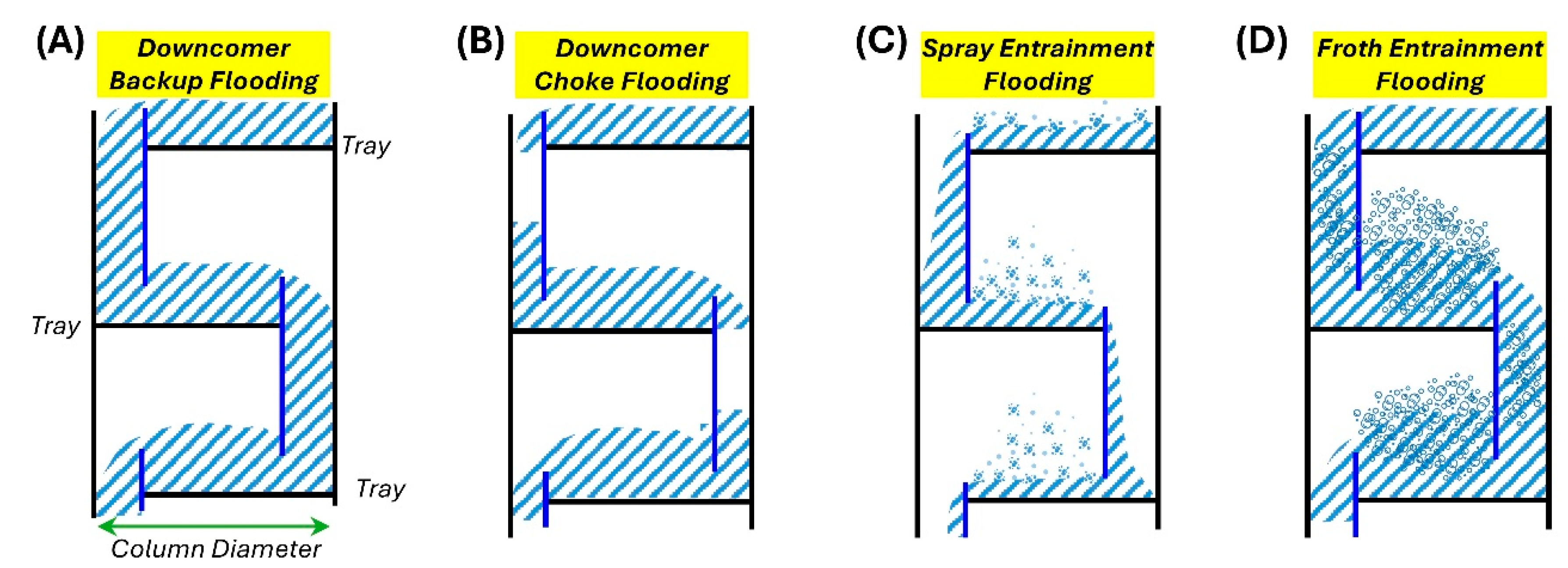
22] suggests a 75% approach to flooding is a good value for various chemical systems. There are four main mechanisms of flooding as shown in
Figure 3. Downcomer backup flooding (
Figure 3A) occurs when the liquid is backed-up into the downcomer due to tray pressure drop, which is usually caused by short tray spacing [
16,
22]. Downcomer choke flooding (
Figure 3B) occurs when the entrance to the downcomer is too narrow resulting in build-up of excesses friction losses for the liquid to overcome [
16]. Spray entrainment flooding (
Figure 3C) occurs when there is a relatively low amount of liquid on the tray because of relatively short weir height and narrow downcomer clearance [
16]. Froth entrainment flooding (
Figure 3D) occurs when significant height of froth reaches the tray above resulting to compromise of the stream concentrations, and this can be a significant effect of settings in the tray spacing, sieve hole diameter, and fraction of the tray allocated for vapor-liquid exchange [
15,
16].
2.3. Notation
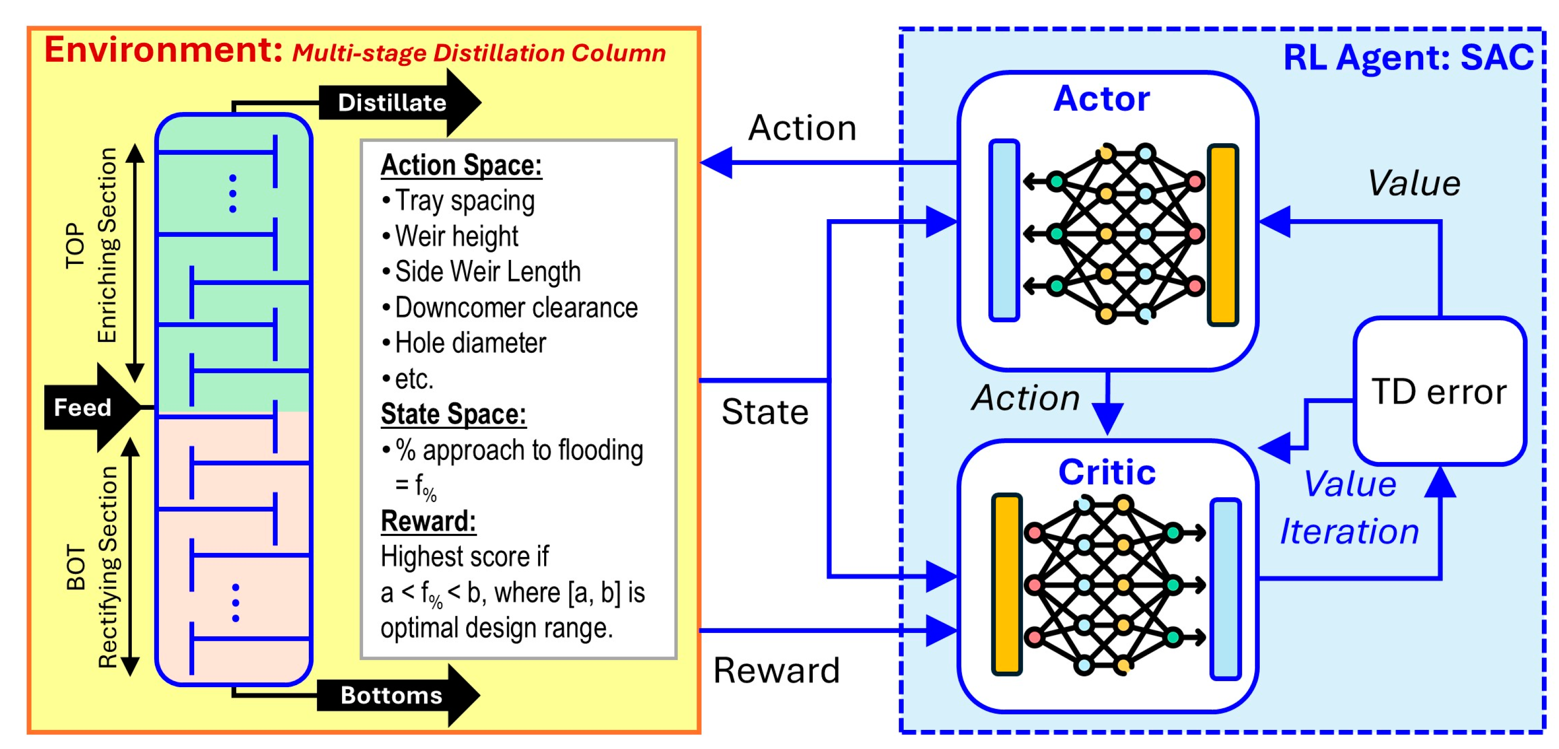
We now present notations to formally define the various components of the task in relation to the established notations in RL. The RL problem at hand is a policy search in a Markov Decision Process (MDP) involving the tuple
. The state space
is a continuous space consists of the following column internal design parameters (
Figure 1 and 2): top section (TOP) % approach to flooding, and bottom section (BOT) % approach to flooding. Note that the state % approach to flooding can be greater than 100% according to distillation column design principles, so
. The action space
is a continuous space consists of the following column internal design parameters (
Figure 1 and 2): tray spacing, weir height, downcomer clearance, weir side length, and hole diameter. The action space is bounded by the allowable values of column design parameters in the AspenPlus software, and the actual values also scale with the units (i.e., ft, cm, or mm; kg or lb; etc.) they are assigned in the software by the user as explained above. The state transition probability
represents the probability density of the next state
given the current state
and action
. The environment (i.e., column internal design) emits a reward
from each transition (i.e., process simulation). Note that this current study also evaluated how various forms of the reward system
may affect the SAC performance.
Table 1 summarizes the variables for the action space and state space with their corresponding description according to the actual settings of the AspenPlus model used in the study. Also refer to
Figure 2 for visualization of the action variables defined in
Table 1. The action space
is multidimensional consists of the column design parameters denoted as
as shown in
Table 1. The state space
is two-dimensional consists of
and
(
Table 1). Note that each section of the column, i.e., TOP and BOT, were represented in the action and state spaces even though the design parameters between the sections were similar.
2.4. SAC RL
We present in this section the key equations of the SAC RL algorithm, but the reader should consult the original works [
13,
14,
20] that established this algorithm if more details are needed.
The goal in SAC RL is to determine a policy
which maximizes two components: (1) the expected return
from the rewards
, where
is the trajectory, when the agent acts according to the policy, and (2) the entropy of the policy
, i.e., entropy of the predicted next actions. To achieve this, the policy model
must be estimated by an optimal policy
that is calibrated (via its model parameters) using data collected about from environment [
14]. Policy in this context is a rule used to decide what next actions to take based on the current state of the environment. Specifically,
is a probability distribution over the possible actions
given the current state
of the environment, i.e.,
. The optimal policy
is modeled using deep neural network with network weights
, and this becomes the Actor network. In essence, the main goal in training a SAC RL model can then be expressed generally as:
where
is the expectation,
is the trade-off coefficient for the entropy
term, and
is the discount factor in the value function [
20].
In general, the reward function
depends on the current state
, the action just taken
, and the next state
such that
t. The dependence in the function
is frequently simplified to have dependence only on the state, i.e.,
, or on the state-action only, i.e.,
. The SAC model used in this study used the former model
. One of the two components of the objective function in the SAC RL agent is to maximize the cumulative reward over a trajectory
and this cumulative reward is commonly called the return
. It has been shown that a discounted return helps in the convergence of RL models, so this is also adopted in the SAC learning model such that
, where
is the discount factor [
14].
The maximum entropy term
(second term in Equation 1) is the unique feature of the SAC RL. By design, this term encourages the RL model to still explore as it learns to prioritize actions with projected high rewards [
14]. This prevents the model from being focused on sub-optimal actions [
23].
The determination of the best actor network
is achieved by using value feedback from a system of Critic networks (see
Figure 1), which are also deep neural networks, that implement double Q-learning [
14]. SAC concurrently learns the policy
, and two Q-functions
and
of the Critic, where
and
are the network weights of the critic networks.
The smoothing constant,
, is a hyperparameter that controls updating the weighs in of the target networks for the Q-functions
and
[
24]. In notation:
; and
.
The fourth hyperparameter to be evaluated is the ‘replay buffer length’, which originates from using replay buffer as a solution to extract more information from the history sequential data for RL training [
24]. Replay buffer is a component of the computation of the target Q-functions
and
presented above. The replay buffer is a finite sized (replay buffer length) memory data. The buffer is created by sampling transitions from the environment according to the exploration policy and the tuple
is stored in the replay buffer. The buffer eventually is filled as more tuple entries are added. When the buffer length is reached, the oldest samples are discarded while maintaining the buffer length. At each timestep the actor and critic are updated by sampling a minibatch uniformly from the buffer.
2.5. Implementation: OpenAI Gymnasium, PyTorch
To eliminate the need to create our custom RL environment, we used the prebuilt RL module called “Gymnasium” by OpenAI [25,26]. This module implements the necessary algorithms and functions to define variable spaces and efficient action space-sampling mechanisms to ensure that RL models are exposed to a wide variety of scenarios resulting to improved learning performance [25,27]. The Python codes are based on the prior work by
2.5.1. Action Variables
Since all action variables in are continuous, these were defined using the ‘Gymnasium.Box()’ function, which is designed to handle tensor of continuous variables. The lower and upper bounds of these action variables were required arguments in the ‘Gymnasium.Box()’ functions.
2.5.2. State Variables
Defining the state space was very similar to how the action space (section 2.5.1) was defined using the ‘Gymnasium.Box()’ function.
2.5.3. Reward Scheme
The reward schemes studied are summarized in
Table 2. Reward is based on the flooding level
of each column section and the scheme for awarding the reward values. Previous works have demonstrated that reward scheme can significantly affect the performance of RL algorithms [28,29,30,31]. The unique aspect of the reward schemes adopted for this study is the separate computation of reward for each column section
, and then aggregating these by summation (weighted and unweighted) into a single reward value
(
Table 2). Scheme 1 and Scheme 2 are built on a model that computes the penalty for deviating from the target state by taking difference of the target state value(s) and the current value of the state [31]. Scheme 3 and Scheme 4 are based on the concept of dividing the state values according to ranges and assigning the highest score on the target range while assigning decreasing reward score was the binning range moves away from the target range. Scheme 5 is built on top of a binary reward system; hence, it represents a binary scheme. The coding of these reward schemes were done in the environment definition via Python scripting.
2.5.4. Hardware Setup
The computer specifications are the following. Unit: Dell Precision 7670 Mobile Workstation; CPU: Intel Core i7-12850HX, 25MB Cache, 24 Threads, 16 Core, 2.1GHz-4.8GHz; Memory: 64GB DDR5; GPU: NVIDIA GeForce RTX 3080Ti with 16GB GDDR6. All computational work done were implemented in this laptop computer running the AspenTech version 12 software suite containing the AspenPlus®, and Anaconda Navigator version 2.5 software [32] containing Python version 3.10 and all the necessary Python packages such as PyTorch (CUDA-enabled), Gymnasium by OpenAI, and the pywin32 package [19] that interfaces with Windows to access the AspenPlus® file. Note that even though this study used a GPU-enabled computer to accelerate PyTorch computations, a CPU-only implementation of PyTorch can still accomplish the computations but at slower computation speeds. Nonetheless, the computations in this work do not require specialized computer hardware beyond a typical hardware requirement for running the AspenPlus® software.
2.5.5. Code and Documentation of the Work Done
The necessary codes used in this work have been organized and stored in an online repository via GitHub as detailed in the Data Availability section. There are two main code files: (1) a Python class file that defines all functions used to read data from (output data) and write data to (input data) AspenPlus® via Python, and (2) Jupyter Notebook files that document the implementation of the SAC RL.
2.6. SAC RL Runs
Since RL training is very sensitive to randomization of the initial weight in the deep neural networks in the actor and in the critic components of the SAC model, a set of ten runs was implemented for each learning setting. Each run has a unique random number generator (RNG) index value used for all PyTorch computations, which consequently fixed the random number used in initializing the weights of the neural networks. The ten unique RNG indices can be seen in the accompanying Jupyter Notebook files in the project online repository (see Data Availability section). This deliberate randomization using known RNG indices accomplishes two crucial tasks: (1) testing the robustness in SACR RL models, and (2) allowing for the repeatability of the randomized runs and results.
All runs were set to a maximum of 500 iterations per SAC learning run, where each iteration consists of one cycle of SAC model reading the current state and reward values of the environment (column model in AspenPlus®), SAC model making prediction for the next actions, and sending the predicted actions to the environment for simulation (to get the next state and reward for next cycle). Even though the traditional fields implementing RL (e.g., computer science, robotics, etc.) would usually set maximum iterations up to the range of millions [
13], distillation column design iteration becomes impractical if the maximum iterations become very high, so our setting of a maximum of 500 iterations per SAC learning run was based on practical basis. The data collected from each run as discussed above would not require extensive downstream processing as these data by themselves are sufficient to evaluate the performance of SAC RL.
Furthermore, each run started with an untrained SAC RL model. This design of the study aimed to demonstrate that even an untrained SAC RL model can learn to optimize within a reasonable length of time (max of 500 iterations).
2.7. Data Collection and Analysis
There were numerous data that could be collected in this study because the nature of the environment is highly data-intensive inherent in computer-based design of distillation columns in AspenPlus®, and because the SAC RL training is data-intensive. This prompted the research team to focus collecting only on key data that would enable evaluation of the performance of SAC RL in column internals design. The data for following variables were saved and used for discussion: levels of the action variables, levels of the state variables, levels of the reward variables, and runtime per iteration. The saving of these data sets were coded in the run codes to eliminate user errors and streamline the analysis.
3. Results and Discussion
The results are presented in the following order:
Section 3.1 covers the results to demonstrate the feasibility of using SAC RL for distillation column design; section 3.2 shows the effect of reward scheme on the performance of SAC RL; section 3.3 discusses the effect of column diameter on the performance of SAC; section 3.4 shows the effect of SAC hyperparameters setting on its performance; and section 3.5 covers the comparison of SAC RL with established optimization algorithms.
3.1. Feasibility of Using SAC RL for Distillation Column Internals Design
The first question that must be answered is “Does SAC RL work as automation method in optimizing distillation column internals design?” The answer is yes, it works, but there are pertinent trends in its performance that must be addressed as we now cover as we proceed. The evidence for this claim can be seen in
Figure 4 and
Figure 5, which were the results when SAC RL was implemented on the column with fixed uniform (in both TOP and BOT sections) diameter of 6-feet. Using the reward Scheme 1, the SAC model learned how to optimize the column design as the training progressed and converging to predicting column designs that maximize the reward (max of 200) as seen in
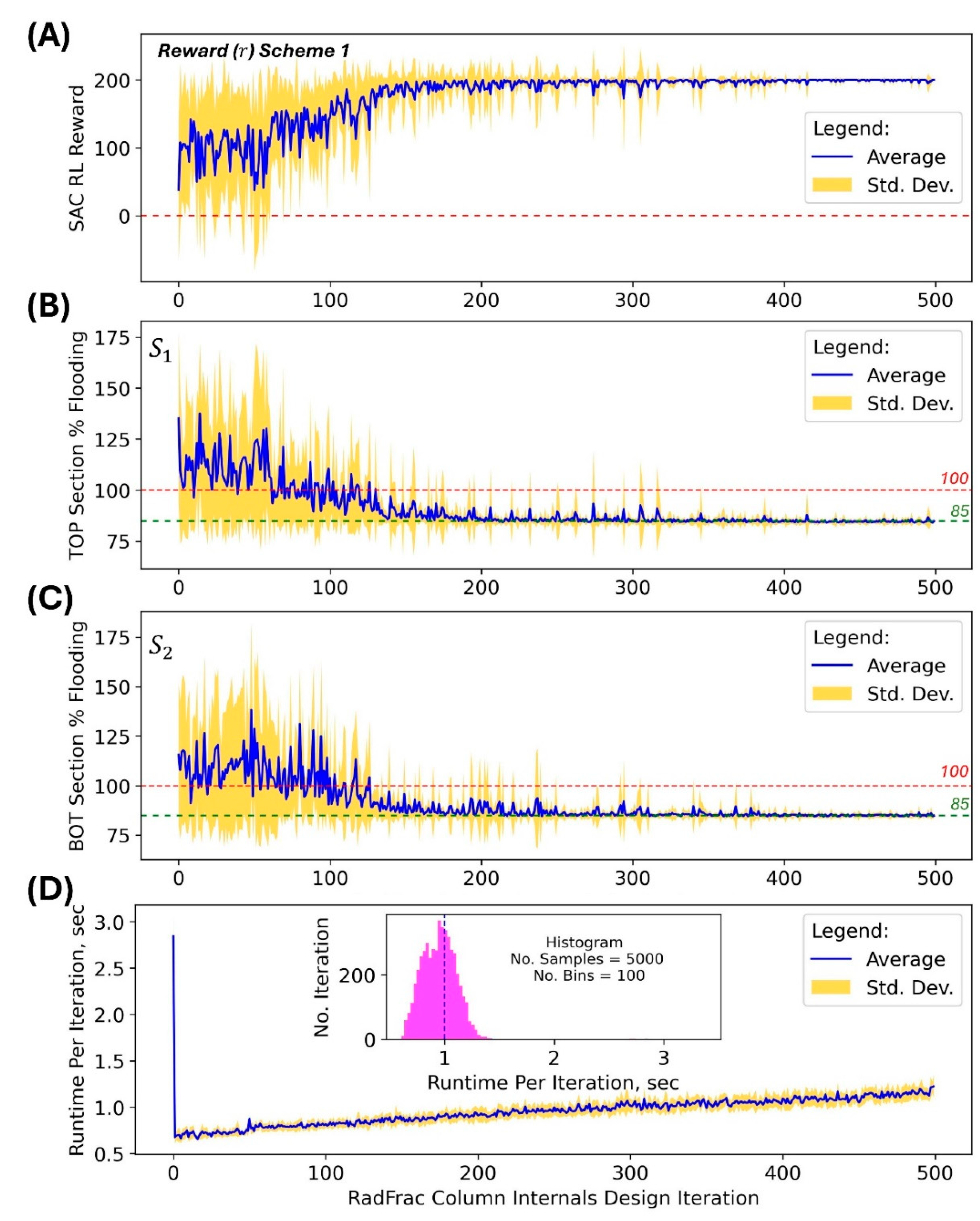
Figure 4A, and selecting actions (column design parameter levels) that resulted to % flooding within the target range of 80-90% (
Table 2 Scheme 1) as seen in
Figure 4B and 4C. Initially, the SAC model does not have any optimal policy in determining the best next actions because the deep neural networks in the critic and actor components were randomly initialized. This is evident in the very large standard deviation of the reward values and state variable values at the beginning of the training (
Figure 4A, 4B, and 4C). However, as the cycle of training-prediction-implementation steps progresses, the model learns the best actions that result to high rewards and the bad actions that result to low rewards, and eventually converges to optimal policies (actor and critic) that favor prediction of actions (
Figure 5) that result in favorable
values resulting to highest rewards (
Figure 4). This trend of convergence is very evident in the last 100 iterations, i.e., 400-500 iteration steps accompanied by smaller (narrower) standard deviation of reward and state variable values (
Figure 4).
Another crucial aspect of the design task is the duration of the SAC RL automated optimization because chemical process design can be time sensitive [
3]. The summary of runtime (in seconds) as shown in
Figure 4D indicates that the average time per design iteration by the SAC model is 1 second (on the laptop computer used in this study – see section 2.5.4 Hardware Setup for details on the computer). This means that a single run with a maximum of 500 iterations (
Figure 4) takes only around 10 minutes, which may be significantly lower than the time it takes to manually iterate the design.
With the numerous iterations that resulted in
values within the target range [80%, 90%) as shown in
Figure 4B and 4C, the SAC-based optimization essentially exhaustively discovered numerous ways on how the column internal parameters can be set while achieving target design specification, i.e.,
. The action space trends shown in
Figure 5 show the corresponding column design parameters for these design iterations that meet design specification.
3.2. Effect of Reward Scheme on the Performance of SAC
There are evidence in the literature of RL algorithms that show the impact of the reward scheme on the performance of RL models [25-27], and this was evaluated in the study. The results in testing the effects of the reward schemes (
Table 2) are summarized in
Table 3. The data in
Table 3 was calculated using the results of the last 100 iteration steps (iteration steps 400 to 500) in each of the ten runs. The idea behind this data analysis is that the learning of the SAC RL model should be improving as it progresses in the sequence of iterations and that the best version of model is achieved towards the end of the learning process. Expectation is based on the proven convergence of SAC RL as more training data is introduced to the model [
13,
14]. Therefore, computing the fraction of these last steps of iterations that meet specific
cut-off would be warranted. Furthermore, the number of steps considered was 100 because the replay buffer length for the SAC model used in these runs is 100.
Looking at the mean and standard deviation results (
Table 3), it can be observed that only Scheme 1, 2 and 3 achieved
values within the target interval [80%, 90%) while Scheme 4 and 5 produced
values above this target range. This supports prior observations in RL models that the reward scheme affects the performance of RL model, even the SAC RL model. An interesting comparison is between Scheme 3 and Scheme 4 because these two schemes are similar in terms of the binning intervals of the
values but with Scheme 4 reward values 10 times lower than those of Scheme 3 reward values. This means that the scaling of the reward values significantly affects the performance of SAC RL model.
The consequence of the effects of the reward scheme is also evident in the fraction of the iterations that meet cut-off values of the design metric
(
Table 3). The best-performing reward schemes Scheme 1, 2 and 3 predicted column design specifications with
around at least 0.80 fraction of the iterations. The poor-performing schemes predicted column design specifications with
at low fractions: ~0.50 for Scheme 4, and ~0.35 for Scheme 5. Scheme 5 that represents a ‘binary scheme’ is the worst reward scheme.
3.3. Effect of Column Diameter on the Performance of SAC
With the positive results of implementing SAC RL as shown in the previous section, it was imperative to evaluate the limitation of the approach, and a direct way of accomplishing this is by varying the diameter of the column. This is because column flooding is inversely proportional to column diameter as shown in theory of distillation column design [
2,
15,
16], i.e.,
. One set of experiments used fixed column diameter values, 5 ft, 6 ft, and 7 ft; and another set included the column diameter (
) in the action space used by SAC RL model. The results of implementing SAC RL in these experiment settings are shown in
Figure 6.
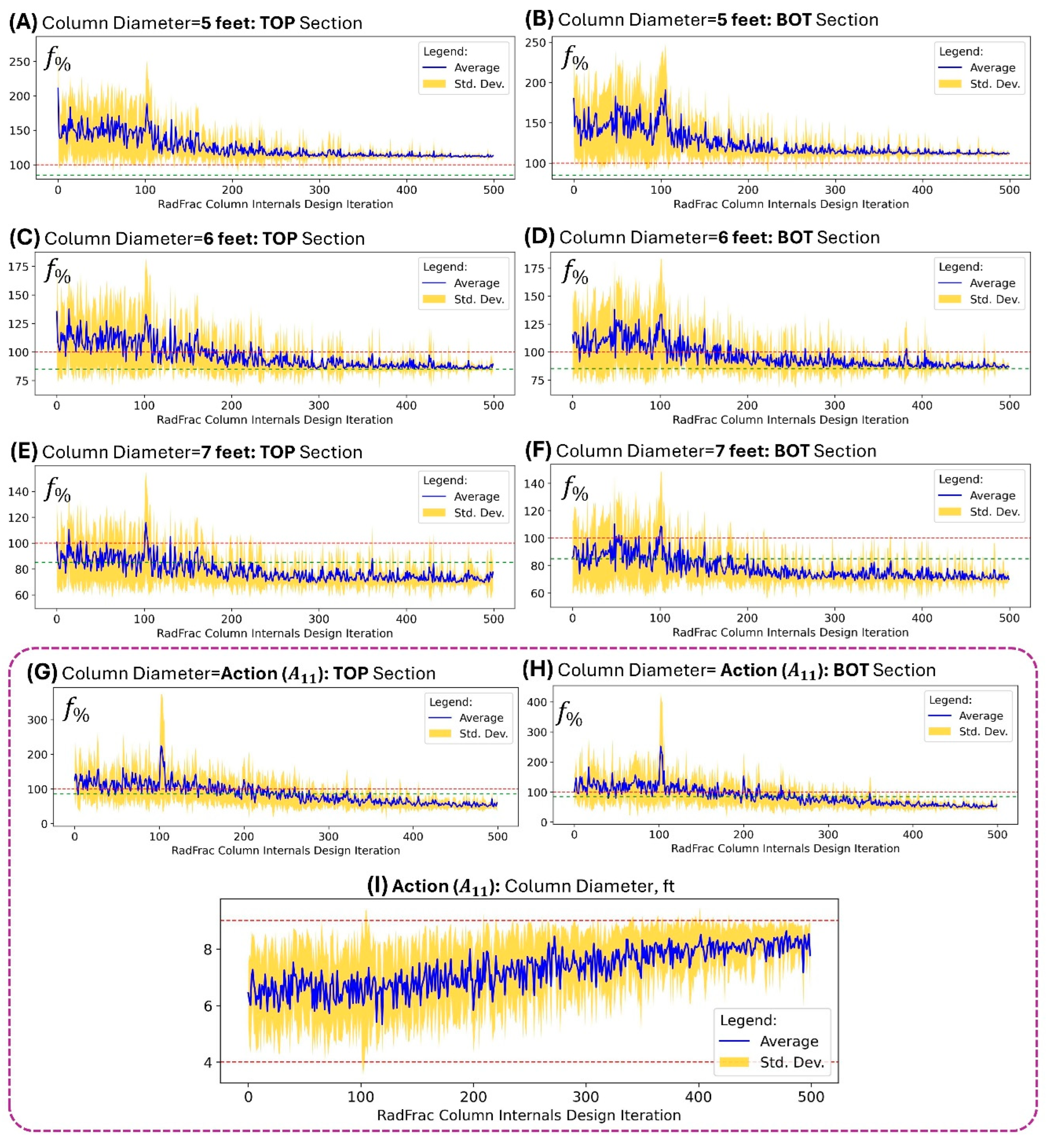
It can be seen in
Figure 6 that the SAC RL converges in terms of its reward values and the resulting state variable values as model training progresses across all column diameter settings. In general, the flooding levels
decrease as the column diameter increase. This is consistent with the theoretical relation that
in inversely proportional to column diameter (relation shown above). When the column diameter is lowest at 5 feet, the converged SAC RL model was just approaching 100% flooding from above (
Figure 6A and 6B) with actual values reaching only ~110% flooding as the lower limit. This means that it is impossible to have a 5-ft column that can operate at the target [80%, 90%) range of
. This impossibility can be quickly checked by implementing the SAC RL as was done here instead of the user spending a very long time manually iterating for something that cannot happen (if column diameter is fixed at 5 ft).
At this point, it is imperative to ask the question “If the flooding
is inversely proportional to column diameter, then why not just keep on increasing the diameter?” The answer comes from the limitations of fluid dynamics in the column when diameter is set too large. The issue of ‘weeping’ can occur when there is a large pool of liquid on the tray (due to large column diameter) while vapor pressure is too low due to larger active area of vapor-liquid contact resulting from larger diameter [
2,
15]. This study does not cover solving the issue of weeping (it can be covered in a future extension of SAC RL in a similar approach). This then begs the question “How was this trade-off in column diameter and flooding included in the SAC RL model?” This trade-off was included by implementing a specialized reward scheme by modifying reward Scheme 1 (
Table 2) as follows and let us call this Scheme 6 for quick referencing:
where
,
and
is the reward in section
of the column. For each
:
where
.
This reward Scheme 6 uses the maximum and minimum possible values of the column diameter, i.e., [4 ft, 9 ft] to compute a scaling factor adjusted to a magnitude of 100 as maximum but assigned a negative value, i.e.,
, to penalize the reward
when the predicted action value for column diameter
gets too large. In essence,
is a penalty value that becomes more negative as column diameter increases. This Scheme 6 bounds reward
resulting in the convergence of the SAC RL model as shown in
Figure 6G, 6H, and 6I.
3.4. Effect of SAC Hyperparameters on Performance
Inherent in training RL models is the tuning of hyperparameters in order to further refine the models. This section covers the results in evaluating the effect of four hyperparameters:
,
,
, and reply buffer length. Of the numerous hyperparameters, these four have direct effects on SAC RL because of their roles in the fundamental equations of SAC.
Table 4 summarizes the flooding results for the top section (TOP) of the column set at fixed diameter of 6 feet. Even though data were also collected for the bottom-section (BOT) of the column, space limitations in the manuscript prompted reducing the presented data to half; hence,
Table 4 shows data for TOP section.
The effect of hyperparameter
can be seen by first comparing the results between Setting 10 and 11, between Setting 7 and 8 (
Table 4). The general trend is that a lower
value of 0.1 will produce higher fractions of runs that fall within the target condition
compared when
is set higher at 0.5. However, when comparing between Setting 8 and 9, it can be seen that
has lower fraction
compared to
. This means that there is an optimal value for
in the range 0.1 to 0.5, and this value may be close to 0.2. Since the value of
is a measure of the fraction of entropy contribution in the loss function (see Equation 1), this observed trend means that the term in the loss function for maximizing entropy should not be zero but it should also be not very large part of the loss function. This is just a fitting observation because this entropy term is a unique feature of the SAC in comparison to other RL algorithms implementing actor-critic networks [
13,
23].
The effect of hyperparameter
can be seen by first comparing results between Setting 3 and 10, and between Setting 4 and 12 (
Table 4). Both pairs show that lower value of
results to higher fraction
. If there is any optimum value somewhere, these data pairs cannot support such possibility – perhaps a more extensive scan of the hyperparameter space can discover an optimum but this is beyond the scope of this study. Since hyperparameter
represents the smoothing coefficient for the target Q-functions, setting its value to zero may not be a good idea because this number controls the update of the Q-function deep neural network weights.
The effect of hyperparameter
can be seen by first comparing results between Setting 1 and 2, between Setting 4 and 5, and between Setting 12 and 13 (
Table 4). It can be seen in these pairs that the trends for fraction
do not follow a clear consistent trend. It is possible that there are confounding effects in the SAC RL training that cannot be easily isolated to be sole effect of
. Therefore, there is no conclusive trend for the effect this hyperparameter based on data.
The effect of hyperparameter ‘replay buffer length’ can be seen by first comparing results between Setting 2 and 4, between Setting 6 and 13, and between Setting 8 and 11 (
Table 4). It can be seen in these pairs that the trends for fraction
do not follow a clear consistent trend. Similar to hyperparameter
, it is possible that there are confounding effects in the SAC RL training that cannot be easily isolated to be sole effect of ‘replay buffer length’. Therefore, there is no conclusive trend for the effect this hyperparameter based on data.
3.5. Comparison of SAC RL Algorithm with Established Optimization Algorithms
A pertinent question at this point is “How does SAC RL performance compare with established optimization algorithms?” This question is necessary to answer because this study is proposing to use SAC RL in optimization task, which has been heavily studied [
33]. The tested algorithms are the following: Nelder-Mead [
34], Broyden–Fletcher–Goldfarb–Shanno (BFGS) [
35], Sequential Least Squares Programming (SLSQP) [
36], Dual Annealing [
37], and simplicial homology global optimization (SHGO) [
38], which were implemented using their pre-built functions in the Python module SciPy [
39]. To simplify the comparative analysis, the target flooding of
was used, which was based on the reward Scheme 1 used for SAC RL. Each algorithm was implemented ten run times with each run assigned with a unique RNG index.
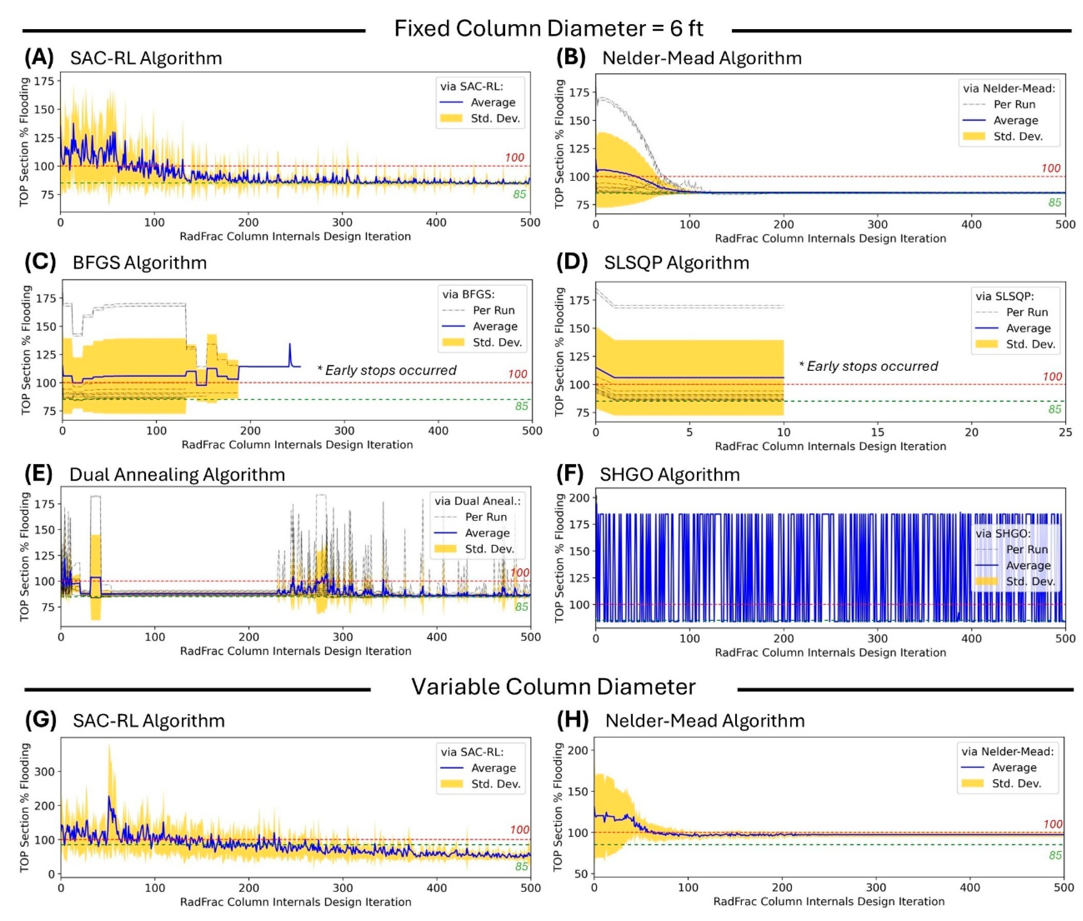
Figure 7 summarizes the results of grouped in two (1) at fixed column diameter of 6 ft as shown in
Figure 7A-7F, and (2) at variable column diameter with penalty on the diameter the same as that of Scheme 6 as shown in
Figure 7G-7H.
It can be seen that each of the algorithms tested exhibited unique performance in terms of optimizing to 85% flooding. Poor performance can be seen for BFGS and SLSQP that exhibited early stops (
Figure 7C and 7D) while dua annealing and SHGO completed the runs but with erratic behavior in various stages of the iterations (
Figure 7E and 7F). The Nelder-Mead exhibited a smooth convergence to the target when the column diameter is fixed (
Figure 7B). However, Nelder-Mead failed to converge to the target when the column diameter was included in the varied parameters (
Figure 7H). We also want to note that Dual Annealing and SHGO were also tested when the column diameter was varied but these algorithms exhibited erratic performance and failed to converge to the target. The SAC-RL algorithm was able to converge to the target in both the fixed column diameter (
Figure 7A) and variable column diameter (
Figure 7G) design scenarios. These trends show the advantage of SAC RL over established optimization algorithms for the task of optimizing distillation column internals design. Due to SAC RL’s maximum entropy term, it continuous to explore as it learns resulting to prevention of exploitation of actions that may be sub-optimal.
4. Conclusions
This study focused on developing an automated method using soft actor-critic (SAC) reinforcement leaning for optimizing the design of distillation column, and this aim was achieved as supported by the results. The integration of SAC RL into AspenPlus® model optimization was achieved by using Python codes written to allow a cyclic interaction between the distillation column model AspenPlus® and the SAC model in PyTorch. The specific chemical system used as case study is a binary mixture of ethanol-water, and the RadFrac module in AspenPlus® was used to enable rigorous column internal design. The results clearly support the following findings: (1) SAC RL works as automation approach for the design of distillation column internals, (2) the reward scheme in the SAC model significantly affects SAC performance, (3) column diameter is a significant constraint in achieving column internals design specification in flooding, and (4) SAC hyperparameters have varying effect on SAC performance.
This study also demonstrated that an untrained SAC RL model can quickly learn how to optimize the design of a distillation column. This means that the algorithm can be implemented as one-shot RL for column internals design. This has significant implications for possible future implementation of the technique as integral part of computer-based chemical process modeling, e.g., if this technique becomes part of AspenPlus® software (and other similar computer packages). That is, there is no need to install a pre-trained SAC RL model into a computer-based chemical process simulation package that would utilize this technique.
Author Contributions
Conceptualization, D.L.B.F., H.B., R.W., C.B., and A.P.M.; methodology, D.L.B.F. and H.B.; software, D.L.B.F. and H.B.; formal analysis, DLBF, A.P.M., M.A.B., and M.E.Z.; investigation, D.L.B.F., H.B., R.W., and C.B.; resources, M.A.B. and M.E.Z.; data curation, D.L.B.F. and H.B.; writing, D.L.B.F., H.B., and A.P.M.; project administration, D.L.B.F.; funding acquisition, D.L.B.F. and M.E.Z. All authors have read and agreed to the published version of the manuscript.
Funding
This research was funded by two grants: (1) LURA Grant by the Louisiana Space Grant Consortium (LaSPACE) with subaward number PO-0000277305 under primary NASA grant number 80NSSC20M0110, and (2) LaSSO Grant by the Louisiana Space Grant Consortium (LaSPACE) and Louisiana Sea Grant (LSG) with subaward number PO-0000277330 under primary NASA grant number 80NSSC20M0110.
Data Availability Statement
All Python codes, Jupyter Notebook files, AspenPlus® model files, sample raw data in spreadsheet, and sample graphics used in the paper are archived online in the project GitHub repository [
40]:
https://github.com/dhanfort/aspenRL.git. This is an open-access repository under MIT License. The reader is encouraged to contact the corresponding author if there is a need for more information beyond the open-access materials.
Acknowledgments
We acknowledge the support of the staff of the Energy Institute of Louisiana (EIL): Sheila Holmes and Bill Holmes. EIL facilities have been instrumental in completing this work.
Conflicts of Interest
The authors declare no conflicts of interest. The funders had no role in the design of the study; in the collection, analyses, or interpretation of data; in the writing of the manuscript; or in the decision to publish the results.
References
- Seidel, T.; Biegler, L.T. Distillation column optimization: A formal method using stage-to stage computations and distributed streams. Chemical Engineering Science 2025, 302, 120875. [CrossRef]
- Seader, J.D.; Henley, E.J.; Roper, D.K. Separation Process Principles: With Applications Using Process Simulators, 4th ed.; Wiley New York, 2016.
- Al-Malah, K.I.M. Aspen Plus: Chemical Engineering Applications, 2nd ed.; Wiley: 2022.
- Haydary, J. Chemical Process Design and Simulation: Aspen Plus and Aspen Hysys Applications; Wiley: 2019.
- AspenTech. AspenPlus. Availabe online: https://www.aspentech.com/en (accessed on.
- 6. Bao J, Gao B, Wu X, et al. Simulation of industrial catalytic-distillation process for production of methyl tert-butyl ether by developing user’s model on Aspen plus platform. Chemical Engineering Journal. 2002 2002/12/28/;90(3):253-266.
- Kamkeng ADN, Wang M. Technical analysis of the modified Fischer-Tropsch synthesis process for direct CO2 conversion into gasoline fuel: Performance improvement via ex-situ water removal. Chemical Engineering Journal. 2023 2023/04/15/;462:142048.
- Syauqi A, Kim H, Lim H. Optimizing olefin purification: An artificial intelligence-based process-conscious PI controller tuning for double dividing wall column distillation. Chemical Engineering Journal. 2024 2024/11/15/;500:156645.
- Byun M, Lee H, Choe C, et al. Machine learning based predictive model for methanol steam reforming with technical, environmental, and economic perspectives. Chemical Engineering Journal. 2021 2021/12/15/;426:131639.
- Schefflan R. Teach Yourself the Basics of Aspen Plus. 2nd ed.: Wiley; 2016..
- Agarwal, R.K.; Shao, Y. Process Simulations and Techno-Economic Analysis with Aspen Plus. In Modeling and Simulation of Fluidized Bed Reactors for Chemical Looping Combustion, Agarwal, R.K., Shao, Y., Eds. Springer International Publishing: Cham, 2024; pp. 17-73. [CrossRef]
- Chen, Q. The Application of Process Simulation Software of Aspen Plus Chemical Engineering in the Design of Distillation Column. In Proceedings of Cyber Security Intelligence and Analytics, Cham, 2020//; pp. 618-622.
- Haarnoja, T.; Zhou, A.; Abbeel, P.; Levine, S. Soft Actor-Critic: Off-Policy Maximum Entropy Deep Reinforcement Learning with a Stochastic Actor. arXiv e-prints 2018, 10.48550/arXiv.1801.01290, arXiv:1801.01290. [CrossRef]
- Haarnoja, T.; Zhou, A.; Hartikainen, K.; Tucker, G.; Ha, S.; Tan, J.; Kumar, V.; Zhu, H.; Gupta, A.; Abbeel, P.; et al. Soft Actor-Critic Algorithms and Applications. ArXiv 2018, abs/1812.05905.
- Wankat, P. Separation Process Engineering - Includes Mass Transfer Analysis, 3rd ed.; Prentice Hall: New York, 2012.
- Kister, H. Distillation Design; McGraw-Hill: Boston, 1992.
- Taqvi, S.A.; Tufa, L.D.; Muhadizir, S. Optimization and Dynamics of Distillation Column Using Aspen Plus®. Procedia Engineering 2016, 148, 978-984. [CrossRef]
- Tapia, J.F.D. Chapter 16 - Basics of process simulation with Aspen Plus∗. In Chemical Engineering Process Simulation (Second Edition), Foo, D.C.Y., Ed. Elsevier: 2023; pp. 343-360. [CrossRef]
- Hammond, M. pywin32. Availabe online: https://pypi.org/project/pywin32/ (accessed on Jan. 9).
- OpenAI. Soft Actor-Critic. Availabe online: https://spinningup.openai.com/en/latest/algorithms/sac.html (accessed on Jan. 9).
- McCabe, W.L.; Thiele, E.W. Graphical Design of Fractionating Columns. Industrial & Engineering Chemistry 1925, 17, 605-611. [CrossRef]
- Jones, E.; Mellborn, M. Fractionating column economics. Chemical Engineering Progress (CEP) 1982, pp 52-55.
- Liu, J.; Guo, Q.; Zhang, J.; Diao, R.; Xu, G. Perspectives on Soft Actor–Critic (SAC)-Aided Operational Control Strategies for Modern Power Systems with Growing Stochastics and Dynamics. In Applied Sciences, 2025; Vol. 15.
- Lillicrap, T.P.; Hunt, J.J.; Pritzel, A.; Heess, N.; Erez, T.; Tassa, Y.; Silver, D.; Wierstra, D. Continuous control with deep reinforcement learning. arXiv e-prints 2015, 10.48550/arXiv.1509.02971, arXiv:1509.02971. [CrossRef]
- Towers, M.; Kwiatkowski, A.; Terry, J.; Balis, J.U.; De Cola, G.; Deleu, T.; Goulão, M.; Kallinteris, A.; Krimmel, M.; Kg, A.; et al. Gymnasium: A Standard Interface for Reinforcement Learning Environments. arXiv e-prints 2024, 10.48550/arXiv.2407.17032, arXiv:2407.17032. [CrossRef]
- Brockman, G.; Cheung, V.; Pettersson, L.; Schneider, J.; Schulman, J.; Tang, J.; Zaremba, W. OpenAI Gym. ArXiv 2016, abs/1606.01540.
- Zhang, X.; Mao, W.; Mowlavi, S.; Benosman, M.; Başar, T. Controlgym: Large-Scale Control Environments for Benchmarking Reinforcement Learning Algorithms. arXiv e-prints 2023, 10.48550/arXiv.2311.18736, arXiv:2311.18736. [CrossRef]
- Nath, A.; Oveisi, A.; Pal, A.K.; Nestorović, T. Exploring reward shaping in discrete and continuous action spaces: A deep reinforcement learning study on Turtlebot3. PAMM 2024, 24, e202400169. [CrossRef]
- Viswanadhapalli, J.K.; Elumalai, V.K.; S, S.; Shah, S.; Mahajan, D. Deep reinforcement learning with reward shaping for tracking control and vibration suppression of flexible link manipulator. Applied Soft Computing 2024, 152, 110756. [CrossRef]
- Veviurko, G.; Böhmer, W.; de Weerdt, M. To the Max: Reinventing Reward in Reinforcement Learning. arXiv e-prints 2024, 10.48550/arXiv.2402.01361, arXiv:2402.01361. [CrossRef]
- Dayal, A.; Cenkeramaddi, L.R.; Jha, A. Reward criteria impact on the performance of reinforcement learning agent for autonomous navigation. Applied Soft Computing 2022, 126, 109241. [CrossRef]
- Anaconda. Anaconda: The Operating System for AI. Availabe online: https://www.anaconda.com/ (accessed on).
- Kochenderfer, M.J.; Wheeler, T.A. Algorithms for Optimization; The MIT Press: Boston, 2019.
- Gao, F.; Han, L. Implementing the Nelder-Mead simplex algorithm with adaptive parameters. Computational Optimization and Applications 2012, 51, 259-277. [CrossRef]
- Fletcher, R. Practical Methods of Optimization; John Wiley & Sons, Ltd: New York, 1987.
- Kraft, D.; Dfvlr, F.B. A software package for sequential quadratic programming; 1988. English. (Forschungsbericht / Deutsche Forschungs- und Versuchsanstalt für Luft- und Raumfahrt, DFVLR; 1988:28).
- Xiang, Y.; Sun, D.Y.; Fan, W.; Gong, X.G. Generalized simulated annealing algorithm and its application to the Thomson model. Physics Letters A 1997, 233, 216-220. [CrossRef]
- Endres, S.C.; Sandrock, C.; Focke, W.W. A simplicial homology algorithm for Lipschitz optimisation. Journal of Global Optimization 2018, 72, 181-217. [CrossRef]
- Virtanen, P.; Gommers, R.; Oliphant, T.E.; Haberland, M.; Reddy, T.; Cournapeau, D.; Burovski, E.; Peterson, P.; Weckesser, W.; Bright, J.; et al. SciPy 1.0: fundamental algorithms for scientific computing in Python. Nature Methods 2020, 17, 261-272. [CrossRef]
- Fortela, D.L.B. aspenRL: Enhanced AspenPlus-based Multi-stage Distillation Design Using SAC Reinforcement Learning. Availabe online: https://github.com/dhanfort/aspenRL (accessed on Jan. 19).
Figure 1.
Schematic of the implementation of soft actor-critic (SAC) RL algorithm in the optimization of column internals design in multi-stage distillation column. The Environment box is separate from the SAC RL model box, but there exists a mechanism for the environment to be observed by the SAC RL to collect the environment’s state and reward and mechanism for the SAC RL model to apply actions to the environment.
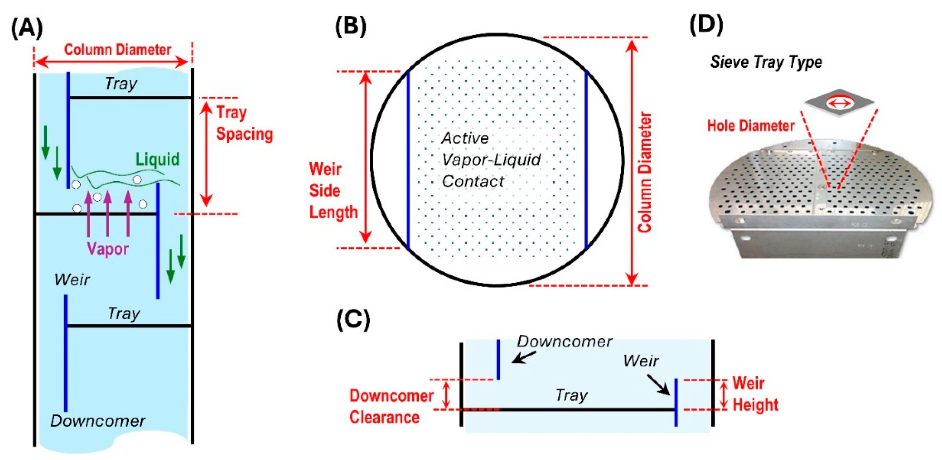
Figure 2.
Distillation column internals design parameters studied for the application of SAC. (A) cross-section view of a vertical section of the column indicating the parameters column diameter and tray spacing, (B) top-view on a tray indicating the parameters weir side length and column diameter, (C) view indicating the parameters downcomer clearance and weir height, and (D) view of a sieve tray indicating parameter hole diameter.
Figure 3.
Distillation tray flooding mechanisms. (A) downcomer backup flooding, (B) downcomer choke flooding, (C) spray entrainment flooding, and (D) froth entrainment flooding.
Figure 3.
Distillation tray flooding mechanisms. (A) downcomer backup flooding, (B) downcomer choke flooding, (C) spray entrainment flooding, and (D) froth entrainment flooding.
Figure 4.
Performance of implementing SAC RL to optimize distillation column internals design by using the reward Scheme 1 for a maximum of 500 iterations. The distillation column diameter was fixed at 6 feet. Ten runs were implemented with each run having its unique RNG index. The following SAC RL model settings were used:
,
,
, and
. (A) SAC RL reward value, (B) column TOP section % flooding level, (C) column BOT section % flooding level; and (D) runtime in seconds per SAC RL iteration. The associated actions (column internal design levels) predicted by the SAC RL model are shown in the next figure (
Figure 5).
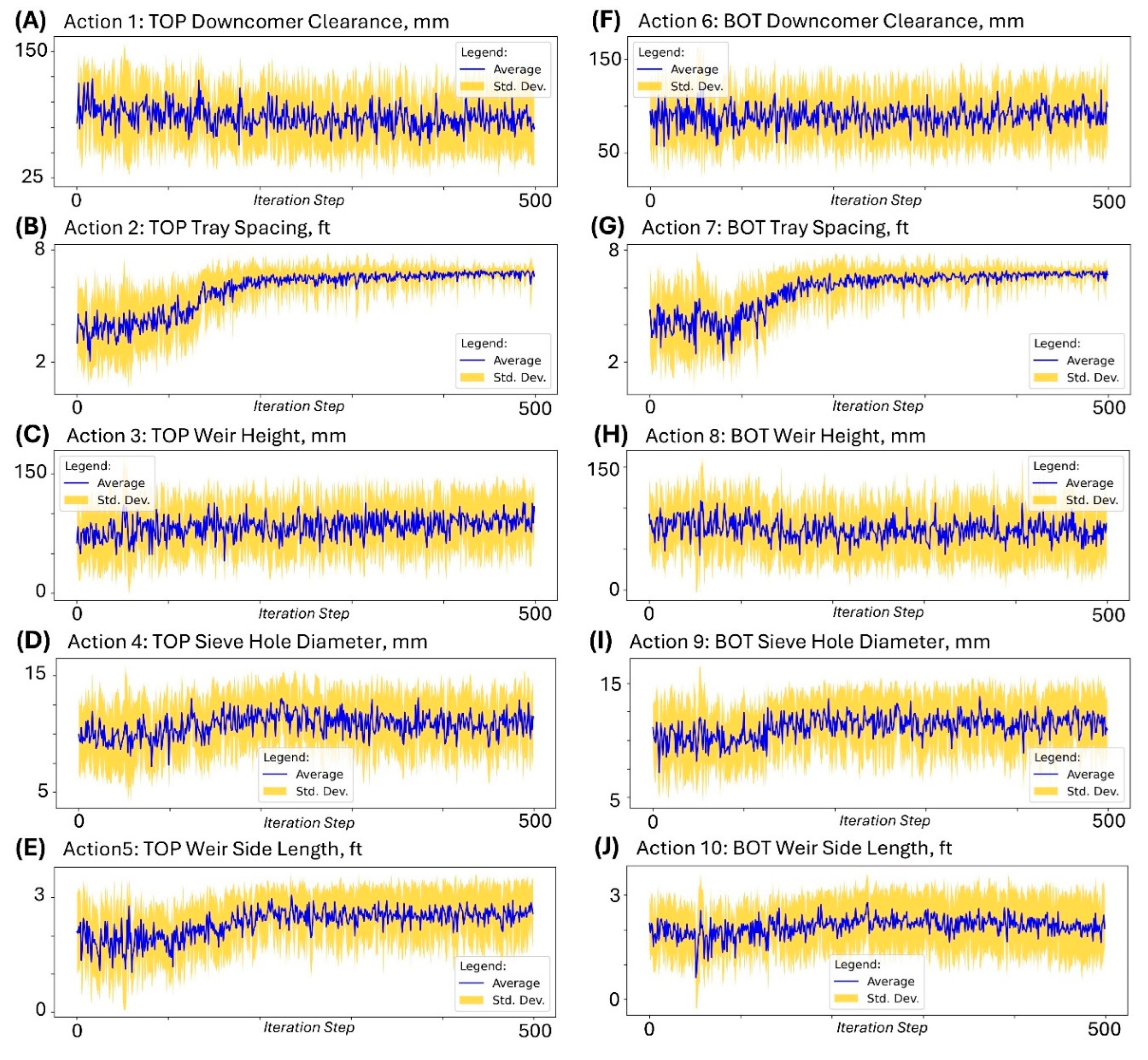
Figure 5.
Actions (column internal design levels) predicted by the SAC RL model as it learns the best policies to optimize the reward. Ten runs were implemented with each run having its unique RNG index. The following SAC RL model settings were used: , , , and . (A) Action 1 () = TOP Downcomer clearance, (B) Action 2 () = TOP Tray spacing, (C) Action 3 () = TOP Weir height, (D) Action 4 () = TOP Sieve hole diameter, (E) Action 5 () = TOP Weir side length, (F) Action 6 () = BOT Downcomer clearance, (G) Action 7 () = BOT Tray spacing, (H) Action 8 () = BOT Weir height, (I) Action 9 () = BOT Sieve hole diameter, and (J) Action 10 () = BOT Weir side length.
Figure 6.
Flooding results when SAC RL was implemented at varied column diameter levels. (A) TOP at 5 ft diameter, (B) BOT at 5 ft diameter, (C) TOP at 6 ft diameter, (D) BOT at 6 ft diameter, (E) TOP at 7 ft diameter, and (F) BOT at 7 ft diameter. When column diameter is in action space as of SAC RL: (G) TOP flooding, (H) BOT flooding, and (I) column diameter predictions by SAC RL.
Figure 7.
Comparing performance of SAC-RL algorithm with that of established optimization algorithms using the reward Scheme 1 as basis for target of optimization to at most 85% approach to flooding. Ten runs were implemented for each algorithm with each run having a unique RNG index. With fixed distillation column diameter of 6 ft: (A) via SAC-RL, (B) via Nelder-Mead, (C) via BFGS, (D) via SLSQP, (E) via Dual Annealing, and (F) via SHGO. With variable distillation column diameter of in the range 4 ft to 9 ft: (G) via SAC-RL, and (H) via Nelder-Mead.
Table 1.
Summary of action and state variables used in the study.
Table 1.
Summary of action and state variables used in the study.
| Action/State Variable |
Description |
|
) = TOP Downcomer clearance |
Distance between the bottom edge of the downcomer and the tray below; Value range: [30, 150]; Units: mm |
|
) = TOP Tray spacing |
Distance between two consecutive trays; Value range: [1, 7]; Units: ft |
|
) = TOP Weir height |
Height of a tray outlet weir, which regulates the amount of liquid build-up on the plate surface; Value range: [10, 150]; Units: mm |
|
) = TOP Sieve hole diameter |
Diameter of the holes on the sieve tray; Value range: [5, 15]; Units: mm |
|
) = TOP Weir side length |
Length of the tray outlet weir; Value range: [0.1, 1]; Units: ft |
|
) = BOT Downcomer clearance |
Distance between the bottom edge of the downcomer and the tray below; Value range: [30, 150]; Units: mm |
|
) = BOT Tray spacing |
Distance between two consecutive trays; Value range: [1, 7]; Units: ft |
|
) = BOT Weir height |
Height of a tray outlet weir, which regulates the amount of liquid build-up on the plate surface; Value range: [10, 150]; Units: mm |
|
) = BOT Sieve hole diameter |
Diameter of the holes on the sieve tray; Value range: [5, 15]; Units: mm |
|
) = BOT Weir side length |
Length of the tray outlet weir; Value range: [0.1, 1]; Units: ft |
|
) = Column diameter** |
Diameter of the column; Value range: [4, 9]; Units: ft |
|
|
; Units: % |
|
|
; Units: % |
Table 2.
Summary of reward schemes used in this study.
Table 2.
Summary of reward schemes used in this study.
| Reward Model |
Definition |
|
Scheme 1
|
:
|
|
Scheme 2
|
:
|
|
Scheme 3
|
:
|
|
Scheme 4
|
is similar to Scheme 3 but with reward values lower by a factor of 10.
:
|
|
Scheme 5
|
:
|
Table 3.
Summary of fractions of column design iterations that are below cut-off values for % flooding values . The last 100 iteration steps of each of the 10 runs was used, i.e., 1000 samples per reward model. The following SAC RL model settings were used: , , , and . Column diameter was fixed at 6 feet.
| Reward Model |
Column Section |
|
|
|
|
|
|
|
Scheme 1
|
TOP |
88.5 |
8.7 |
0.955 |
0.826 |
0.251 |
0 |
| BOT |
88.8 |
8.6 |
0.945 |
0.796 |
0.216 |
0 |
|
Scheme 2
|
TOP |
87.9 |
7.1 |
0.963 |
0.837 |
0.293 |
0 |
| BOT |
88.2 |
6.1 |
0.974 |
0.835 |
0.146 |
0 |
|
Scheme 3
|
TOP |
87.7 |
6.0 |
0.971 |
0.841 |
0.29 |
0 |
| BOT |
88.0 |
5.6 |
0.976 |
0.823 |
0.214 |
0 |
|
Scheme 4
|
TOP |
93.8 |
14.6 |
0.851 |
0.587 |
0.111 |
0 |
| BOT |
94.0 |
14.6 |
0.845 |
0.57 |
0.102 |
0 |
|
Scheme 5
|
TOP |
101.9 |
21.8 |
0.686 |
0.371 |
0.067 |
0 |
| BOT |
102.4 |
22.0 |
0.686 |
0.359 |
0.052 |
0 |
Table 4.
Summary of fractions of column design iterations that are below the cut-off value
Table 4.
Summary of fractions of column design iterations that are below the cut-off value
| SAC Setting |
Hyperparameter |
|
|
|
|
|
|
Replay buffer length |
| 1 |
0.2 |
0.05 |
0.99 |
50 |
0.945 |
85.3 |
4.0 |
| 2 |
0.2 |
0.05 |
0.9 |
50 |
0.918 |
85.9 |
3.6 |
| 3 |
0.5 |
0.05 |
0.9 |
100 |
0.881 |
86.8 |
5.3 |
| 4 |
0.2 |
0.05 |
0.9 |
100 |
0.886 |
86.8 |
6.3 |
| 5 |
0.2 |
0.05 |
0.99 |
100 |
0.826 |
88.5 |
8.7 |
| 6 |
0.2 |
0.01 |
0.99 |
50 |
0.978 |
84.8 |
2.1 |
| 7 |
0.5 |
0.01 |
0.9 |
50 |
0.865 |
86.8 |
5.2 |
| 8 |
0.1 |
0.01 |
0.9 |
50 |
0.881 |
86.7 |
5.1 |
| 9 |
0.2 |
0.01 |
0.9 |
50 |
0.938 |
85.4 |
3.2 |
| 10 |
0.5 |
0.01 |
0.9 |
100 |
0.916 |
86.5 |
5.3 |
| 11 |
0.1 |
0.01 |
0.9 |
100 |
0.947 |
85.8 |
3.2 |
| 12 |
0.2 |
0.01 |
0.9 |
100 |
0.932 |
86.4 |
6.1 |
| 13 |
0.2 |
0.01 |
0.99 |
100 |
0.870 |
87.5 |
7.7 |
|
Disclaimer/Publisher’s Note: The statements, opinions and data contained in all publications are solely those of the individual author(s) and contributor(s) and not of MDPI and/or the editor(s). MDPI and/or the editor(s) disclaim responsibility for any injury to people or property resulting from any ideas, methods, instructions or products referred to in the content. |
© 2025 by the authors. Licensee MDPI, Basel, Switzerland. This article is an open access article distributed under the terms and conditions of the Creative Commons Attribution (CC BY) license (http://creativecommons.org/licenses/by/4.0/).