
Submitted:
21 January 2025
Posted:
21 January 2025
You are already at the latest version
Abstract
This work is a continuation of our recent work on the prediction of hydrogen-bonding (HB) interaction enthalpies [1]. In the present work, a simple method is proposed for the prediction of the HB interaction free energies. Quantum chemical (QC) calculations are combined with the Linear Solvation Energy Relationship (LSER) approach for the determination of novel QC-LSER molecular descriptors and the development of the method. Each hydrogen-bonded molecule is characterized by an acidity or proton donor capacity, , and/or a basicity or proton acceptor capacity. These descriptors suffice for the prediction of HB interaction free energy when the interacting molecules possess one acidic and or one basic site. In this case of two interacting molecules, 1 and 2, their overall HB interaction free energy is , where c is a universal constant equal to (ln10)RT = 5.71 kJ/mol at 25 oC. This holds true over the full composition range, that is, regardless of which molecule is solute and which solvent. In the case of complex multi-sited molecules possessing more than one distant acidic sites and/or more than one types of distant basic sites, two sets of and descriptors are needed, one for the molecule as solute in any solvent and the one for the same molecule as solvent of any solute. Descriptors and are reported for a number of common hydrogen bonded molecules but they may be obtained for any other hydrogen-bonded molecule of interest from its molecular surface charge distribution already available or easily obtained via relatively cheap DFT / basis-set QC calculations. The new predictive scheme is validated against corresponding estimations of the widely used Abraham’s LSER model. The developments in the present work and the previous one are useful for solvation studies in chemical and biochemical systems and, particularly, for equation-of-state developments in molecular thermodynamics. The strengths and limitations of the new predictive method are critically discussed.
Keywords:
Solvation Thermodynamics
; Associating Fluids
; Molecular Conformations
; Sigma Profiles
1. Introduction
The role of hydrogen bonding (HB) in numerous physicochemical processes in biology and life itself, in drug and xenobiotic interaction with biota, in aquatic environments and in chemical industry cannot be overemphasized [2,3,4,5,6,7,8,9,10,11,12]. HB is studied experimentally and theoretically for more than one century now [13]. It is one of the principal causes of mixture non-idealities and is of particular interest in modern molecular thermodynamic developments. The current status in the open literature regarding the estimation of the strength of hydrogen bonding interactions and the open problems are extensively discussed in numerous monographs, reviews and relevant articles [1,2,3,4,9,10,11,14,15,16,17].
At the outset it should be stressed that HB interaction energies and free-energies are obtained indirectly via modelling their contribution to measurable thermodynamic properties and, thus, they are attributed a quasi-thermodynamic character. One of the most exploited thermodynamic properties for extracting HB information is solvation free energy and the associated solute partitioning / transfer and the limited Henry’s law. The solvation free-energy, , and its components enthalpy, and entropy, , are directly connected with phase equilibrium studies involving activity or fugacity coefficients through the following most useful classical working equation for the equilibrium solvation constant :
Vm2 in Equation (1) is the molar volume of the solvent (component 2) and is the activity coefficient of solute 1 at infinite dilution in solvent 2. is the vapor pressure of pure solute at temperature, T, and its fugacity coefficient (typically, set equal to 1 at ambient conditions).
It is from the assumed contribution to quantities like the above solvation free energy and enthalpy that HB interaction energies (enthalpies), , and free energies, , are very often obtained. In this regard, many attempts have been made to model and quantify HB interactions for use in quantitative structure-property and structure - activity relationships (QSPR / QSAR) and in the development of molecular thermodynamic models of highly non-ideal mixtures [11,12,14,15,16,17,18,19,20,21,22,23,24,25,26,27].
One of the most successful QSPR-type approaches is Abraham’s LSER (Linear Solvation Energy Relationship) model [28,29,30,31,32,33] and has led, ultimately, to the valuable and freely available comprehensive and rich in thermodynamic information LSER Database [34].
The LSER model uses simple linearity equations for the quantitative description of solute transfer between two phases. These important linear relationships, in Abraham’s LSER approach, take the form of Equations (2) and (3) for the equilibrium constant, , of solute partitioning between gas and liquid phases and for the corresponding solvation energy (enthalpy) constant, , respectively:
and
The upper-case letters in these equations indicate solute molecular LSER descriptors while the lower-case letters indicate the corresponding complementary but solvent-phase-specific LFER coefficients. The solute molecular LSER descriptors Vx, L, E, S, A, and B, are corresponding to the McGowan’s characteristic volume, the equilibrium constant for the gas–liquid partition in n-hexadecane at 298 K, the excess molar refraction, the dipolarity / polarizability, the hydrogen bonding (HB) acidity A, and hydrogen-bonding basicity B, respectively [28,29,30,31,32,33]. Thus, in Abraham’s LSER model, the HB contribution to solvation energy (enthalpy) constant of a solute 1 by solvent 2 is modelled as the sum, ae2A1 + be2B1. The corresponding HB contribution to the equilibrium constant for the solvation free-energy is modelled as the sum ag2A1 + bg2B1. Analogous to the above equations apply for the solute transfer / partitioning between two condensed phases.
There are three main limitations of this otherwise highly successful LSER model. The descriptors A and B and the coefficients a and b are essentially obtained from extensive experimental data correlations and depend on their availability. In fact, for just a few decades of solvents are a and b coefficients available [17,34,35]. The second limitation arises from the very way this LSER model treats hydrogen bonding. On self-solvation, where solute and solvent become identical, one would expect the acid – base (aA) interaction to be identical to the base – acid (bB) interaction between the very same pair of donor – acceptor sites. However, in LSER the product aA is in general different from bB [40,41,42]. In fact, this is the case for other popular QSPR – type models, including Raevski’s HYBOT model [36]. This restricts rather severely the transfer of this HB information into other models, especially in Molecular Thermodynamics modeling of hydrogen bonding. The third limitation arises from the fact that the LFER coefficients, a and b, are determined simultaneously with all other LFER coefficients, including the constant c, by multilinear regression of available experimental solvation data. This implies that some caution must be exercised when attributing to the above sums, ae2A1 + be2B1 and ag2A1 + bg2B1 sums the (exclusive or total) HB contribution to solvation energy and free energy, respectively.
Recently [1], a predictive method was developed for the HB contribution to solvation energy. The method is using new molecular descriptors [37] based on quantum – chemical (QC) calculations and has a simple structure analogous to Abraham’s LSER model [28,29,30,31,32,33]. The novel set of molecular descriptors, referred to as QC-LSER descriptors, is based on the molecular surface charge densities or σ – profiles widely used by the quantum-mechanics based COSMO-RS model [38,4]. These σ- profiles are available, free of charge, for thousands of molecules in the open literature, as an example in ref. [45]. They may, of course, be obtained also by using appropriate quantum-chemical calculation suites, such as the TURBOMOLE, DMol3 of BIOVIA’s MATERIALS STUDIO suite, or the SCM suite [46,47,48]. In our previous work [1], the σ-profiles from COSMObase [44] at the DFT / TZPVD-Fine level of quantum chemical calculations are used and the corresponding QC- LSER descriptors for a number of common hydrogen bonded solutes were reported.
Two of the QC-LSER descriptors, the HB acidity, Ah, and the HB basicity, Bh, were particularly explored for the development of the predictive scheme due to their sound basis and insightful character [37]. In fact, the effective HB acidity descriptor of a solute was given by the product α = fAAh and the effective HB basicity descriptor by the product β = fBBh. It was observed that the “availability fractions” fA and fB are characteristics of homologous series (have the same value for all solutes of the homologous series). The factors fA and fB and the descriptors α and β were reported for a number of common hydrogen-bonded solutes [1]. With these descriptors, the HB interaction energy for a solute 1 – solvent 2 pair may be obtained at 25 °C by the simple equation:
The method was tested against LSER data (ae2A1 + be2B1) but also against corresponding estimations of from COSMO-RS model [44]. In nearly all cases the predictions were close to one or both of these sets of data.
The present work is attempting to extend this previous method [1] to a simple and versatile method for the prediction of the HB contribution to solvation free-energy, , of solute 1 in solvent 2. This task, however, is not trivial. In contrast to , COSMO-RS does not provide estimations of and there are good reasons for this: Besides the energy (enthalpy) component, has also an entropy component which is not easily amenable to a priori estimation in complex hydrogen-bonded solvent environments. Thus, the developments of the present work will be confined and exclusively based on the corresponding Abraham’s LSER estimations, ag2A1 + bg2B1. It is pointed out again that LSER is currently one of the best predictive models for solvation free energies. The goal of the present work is to attribute effective acidity and basicity descriptors, αG1 and βG1 to each solute, which will enable us to predict their HB contribution to solvation free energy in a solvent with effective acidity and basicity descriptors, αG2 and βG2, by an equation analogous to Equation (4), or:
In this effort, one of the major issues that must be addressed, is the fact that in LSER calculations the quantity is often solvent – specific, especially in multi-sited solvents (molecules with many and/or distant HB sites) or . In contrast to the LSER model may provide estimations of for many more hydrogen-bonded mixtures, including multi-sited solvent systems. This will help reveal the solvent-specific character of in these systems.
The fact that our calculations are heavily based on the corresponding LSER calculations reorients also the central scope of the present work: The LSER model reproduces successfully the experimental solvation data for some decades of hydrogen-bonded solvent systems. The developments in the present work aim, ultimately, at complementing and extending the LSER method to many more solvent systems by removing its above-mentioned drawbacks. The rationale and the structure of the new predictive method are presented in the next section.
2. The Predictive Method for HB Interaction Free Energies
As mentioned above, the developments in the present work will be in line with the corresponding developments in our previous work on HB interaction energies [1]. The effective acidity and basicity descriptors will be obtained by, first, determining the corresponding “availability fractions” fAG and fBG, which will give:
An updated list of QC-LSER descriptors, including Ah and Bh descriptors, are reported in Table SI1 of the Supplementary Information SI1 file. Thus, the first step is the determination of fractions fAG and fBG, mainly, from the corresponding LSER estimation, ag2A1 + bg2B1 [28,29,30,31,32,33] and along the lines of our previous work [1]. In this first step we will focus on relatively simple systems. Complex multi-sited solvent systems, exhibiting solvent – specific peculiarities, will be examined later.
In order to make the presentation of the method clear, let us consider two self-associated compounds, say ethanol (1) and 2-pyrrolidone (2) with corresponding acidity descriptors and , and basicity descriptors βG1 and βG2, respectively. By adapting the rationale of the previous work on HB interaction energies [1] to the present case of HB interaction free-energies, we may write for the pair 1 – 2 HB interaction free energy at 298.15 K the following equation:
The corresponding equations for their self-association interaction in a self-solvation process are:
Let us consider also their interaction with a proton – donor compound 3 (say, chloroform), which cannot self-associate but it can form hydrogen bonds with both compounds 1 and 2. The corresponding equations for their HB interaction free energy are:
Equations (7) to (11) are five independent equations with five unknowns. If all interaction free energies are known, they may be solved, in principle, and give , , βG1, βG2, and .
Alternatively, or in addition, one may use a proton-acceptor compound 4 (say, ethyl acetate), which cannot self-associate but it can form hydrogen bonds with both compounds 1 and 2. The corresponding equations for their HB interaction free energy are now:
Equations (7)–(9), (12) and (13) are five independent equations with five unknowns. If all interaction free energies are known, they may be solved, in principle, and give , , βG1, βG2, and βG4. In principle, the first four descriptors would be identical to the ones obtained above with compound 3. Alternatively, or in addition, one could use another proton acceptor compound 5 (say, tetrahydrofuran) and obtain , , βG1, βG2, and βG5.
The above procedure could be repeated by substituting compound 1 with another compound 6 from the same homologous series (say, 1-butanol in place of ethanol). Solution of the set of the new independent equations would give the descriptors and βG6. What is important now is to closely examine the descriptors of compounds 1 and 6 of the same homologous series (1-alkanols, in our case).
Following our previous practice [1], we may write the following equations for compound 1:
and, similarly, for compound 6:
As mentioned already, the coefficients fAGi and fBGi in the above equations are considered to reflect the effective fractions of the acidity and basicity sites of compound i which are available for hydrogen bonding. For a given HB functional group (-OH, in our case).it is rather reasonable to expect that these effective fractions are close, if not identical, for all members of the homologous series. Thus, the main focus of the above calculation scheme is on the determination of the common average values of fractions fAGi and fBGi in the homologous series of compounds i. For this purpose, many representative interacting compounds were used for each examined compound of the various homologous series and the determined descriptors are reported in Table 1. It is recalled again that the above calculation scheme was heavily based on the estimation of by Abraham’s LSER method [28,29,30,31,32,33], or:
3. Results
In this section we will compare the calculations by Equation (7), using the molecular descriptors of Table 1, with the LSER calculations [17] by Equation (14). The detailed results are assembled in six tables, SII1 to SII6, and are reported in Supplementary Information file SI2. The full list of results with all examined hydrogen-bonded solutes are reported in each of these tables.
Table SII1 contains the results for the solvation in methanol, ethanol and 1-octanol solvents. All three solvents, members of the homologous series of 1-alkanols, are characterized by one single set of availability fractions, namely, fAGi = 0.54 and fBGi = 0.65. The results for solvation in 1-octanol solvent might be improved by using a different set with lower availability fractions but, following our previous practice [1], we have refrained from introducing such refinements at this stage of development of the predictive method. What is essential to notice is that, in this case of relatively simple HB functional groups, the equality holds true.
As observed in Table SII1, in the overwhelming majority of cases, especially in methanol and ethanol solvents, the discrepancies between predicted and LSER estimations of are less than 0.5 kcal/mol (or 2 kJ/mol). The peculiarities with phenols, which were noticed also in our previous work [1], seem to persist in HB contributions to solvation free energy as well. As previously [1], we have refrained from changing their availability fractions until it is clarified that their deviations are not due to rather excessively high HB LSER molecular descriptors.
For the bulk of solutes, only their most stable conformers C0 are reported in Table SII1 and in the rest of tables in SI2 file. For some solutes, however, prone to intramolecular hydrogen – bonding, such as ethoxy-alkanols, more extended conformers are also reported. It is clear from Table SII1 that these conformers, when used with the availability fractions of conformers C0, lead to higher deviations from LSER estimations. This means that they must be attributed their own set of availability fractions if selected to replace conformers C0 in the predictions. Alternatively, as discussed previously [1], relatively large deviations of predictions with C0 conformers may imply that additional solute conformers must be used in order to properly represent its solvation behavior in the studied solvent.
Table SII2 contains the results for solvation in acetic acid, formamide and 2-pyrrolidone solvents. There are two points to be made regarding acetic acid solvent. The selected values for the availability fractions give rather satisfactory results for solvent or solute acetic acid but not as good for its self-solvation. It is not quite clear how the acid dimerization could explain this discrepancy [49]. The second point regards the solvation of 1-alkanols in acetic acid. As observed, the predicted results are higher than the corresponding LSER estimations. But, tt is also observed that the LSER estimations for the case of solvation of acetic acid in 1-alkanols (cf. Table S2) are significantly higher than the corresponding LSER estimations for the solvation of 1-alkanols in acetic acid. It is not quite clear if the tendency for esterification could explain this peculiarity. It should be mentioned, however, that this discrepancy between LSER estimations was also observed previously [1] in the case of HB contributions to solvation enthalpies but it was not in agreement with corresponding COSMO-RS estimations [44]. It should be clarified that the present predictive method accounts for plain HB interactions. Peculiarities of cooperativities, reactions, ionizations or cooperativities [12] are beyond the scope of the method at this stage of its development.
The predicted results for the case of solvation in formamide are rather satisfactory for the bulk of the studied solutes. The selected values for the availability fractions give also satisfactory predictions for the solvation of formamide in various solvents as well as for its self-solvation.
The results for the solvation in 2-pyrrolidone deserve some discussion. The availability fractions for 2-pyrrolidone are (cf. Table 1): fAG = 0.35 and fBG = 0.38. As observed in Table SII2, for nearly all heterosolvated (non-self-associated) proton acceptor solutes, like ethers, esters, ketones, etc. the predicted results are higher than the corresponding LSER estimations. One could consider this discrepancy as an indication of a rather exaggerated high proton-donor capacity of 2-pyrrolidone or an assumed high value for the availability fraction fAG. By lowering its value from 0.35 to a value below 0.15, indeed, satisfactory results could be obtained for these heterosolvated compounds. However, this lowering of fAG would imply a significant increase in fBG above 0.85 in order to retain self-solvation result in satisfactory agreement with LSER estimations. But this alternative pair of availability fractions would lead to rather very high discrepancies for nearly all other studied solutes. Thus, the source of this discrepancy for the heterosolvated solutes is not clear. As in the case of 1-alkanol solvents, the solvation of phenols and carboxylic acids in 2-pyrrolidone exhibits the same type of discrepancies, again, of not clear origin. The case of phenolic / aromatic solutes will be discussed in the next section.
The results for solvation in aniline are reported in Table SII3 along with the results for solvation in chloroform and ethyl acetate. Besides acidity and basicity character, aniline has also an aromatic character. The availability fractions, heavily dictated by its self-solvation, are: fAG = 0.45 and fBG = 0.95. The rather high value of fBG underlines its basic character. For the bulk of solutes, the predictions are in rather satisfactory agreement with LSER estimations. The agreement for carboxylic acids is also satisfactory. Phenols are again an exception. Their discrepancy could be removed by increasing their fBG, but, as argued above, we have refrained from doing so in this work. The solvation results for the solute aniline in the studied solvents are also satisfactory (cf. Tables SII1–SII4).
Chloroform is a proton donor and cannot self-associate (heterosolvated compound). As seen in Table SII3, the availability fraction fAG = 0.37, leads to predictions which are nearly always higher (lower in absolute terms) than the corresponding LSER estimations. One would be tempted, then, to increase fAG in order to improve results. This, however, would deteriorate the results for the solvation of the solute chloroform in the various other solvents and, thus, we have refrained from doing so in this work. In fact, the source of the observed discrepancies may be due to the fact that part of the HB contribution to solvation free energy may be present in the constant LFER coefficient of the LSER model or in some of the other terms of the LSER Equation (1). If this is the case, better agreement with LSER estimations could be reached by simply adding a constant term of the order of 1.2 in the predictions by Equation (7).
Ethyl acetate is a proton acceptor and, like chloroform, cannot self-associate. As seen in Table SII3, the availability fraction fBG = 0.49 leads to predictions in rather satisfactory agreement with LSER estimations for nearly all studied solutes. Similar is the picture with the other proton acceptor heterosolvated solutes like butyl acetate, tetrahydrofuran, diethyl ether, butanone, etc., as one can easily verify by just using Equation (7) with the αG and βG descriptors of Table 1.
Of much interest, however, are the results reported in Table SII4 for the solvation in diethylene and triethylene glycols. As seen, for each of these solvents, two alternative predictions are reported based on the two alternative sets of their αG and βG descriptors reported in Table 1. The very molecular structure of these solvents differentiates their solvent behavior from their solute one, as will be discussed in the next section. For the time being let us focus on the results in Table SII4.
As observed in Table SII4, the predictions based on the “solute” descriptors of the solvent are significantly lower compared to the predictions based on the “solvent-specific” descriptors of the solvent. This is more pronounced for triethylene glycol having the bigger multi-sited molecular structure. As seen in Table SII4, the average deviation in the case of triethylene glycol, using “solute” descriptors, is 8.99 kJ/mol and, when using the “solvent – specific” descriptors, the average deviation is reduced to 0.08 kJ/mol. In the case of diethylene glycol, the average deviation, using the “solute” descriptors, is 5.08 kJ/mol and is reduced to 0.39 kJ/mol when using the “solvent-specific” αG and βG descriptors reported in Table 1. For both glycols, the predictions with the solvent – specific αG and βG descriptors are in rather satisfactory agreement with the corresponding LSER estimations for nearly all studied solutes. Phenols are, again, exceptions with the predictions being lower (in absolute terms) than the LSER estimations, as with all other studied solvents.
Similar comments apply to the results reported in Table SII5 for solvation in solvents ethylene glycol and 1,2 – propylene glycol. In the case of ethylene glycol, the above average deviations are 1.63 kJ/mol with the “solute” descriptors and 0.23 with the solvent – specific descriptors. In the case of 1,2 – propylene glycol, these average deviations are 3.08 kJ/mol and 0.96 kJ/mol, respectively.
In contrast to the organic solvents discussed so far, the solvation in water presents numerous peculiarities and satisfactory agreement of predictions with LSER estimations is rather difficult to obtain with just one solvent – specific set of αG and βG descriptors. By using the “solute” descriptors of water, the deviations are often large, as seen in Table SII6. In nearly all cases, the predictions are lower (in absolute terms) than the corresponding LSER estimations. Part of these deviations might be attributed to the relatively high constant term of Equation (1) in the case of solvation in water [17]. But still the observed discrepancies elude such a simple explanation. The picture that emerges from Table SII6 is pointing to a rather solute – specific source of discrepancy in these aqueous systems. Thus, in Table SII6 are also reported the changes in fBG of solutes required to bring agreement between predictions and LSER estimations. As seen, these changes must often be well above 100%. An attempt to explain these peculiar discrepancies is made in the next section.
4. Discussion
The results presented in the previous section indicate that the prediction of cannot be made with one single set of αG and βG descriptors for all solvents. One single set of αG and βG descriptors (the same set for the compound as solute and as solvent) seems to be sufficient for the organic solvents of relatively simple molecular HB structure, like the solvents in Tables SII1 to SII3 in SI2 file. Organic solvents with more complex molecular HB structure, like the solvents of Tables SII4 and SII5 of SI2 file require two separate sets of αG and βG descriptors, one to account for their HB behavior as solvents and one for their HB capacity as solutes. Water is a stand-alone case in which the above predictive scheme does not seem to apply. The key question is why the prediction of in these solvents require more than one set of αG and βG descriptors. The answer to this question is not trivial but some hints could be drawn from an inspection of the molecular structure of these solvents.
In Figure 1 are shown the geometries and COSMO-surfaces [44] of three representative conformers of triethylene glycol. The open structure of conformer C0 exhibits its two proton donor (acidic) sites as well as its four proton acceptor (basicity) sites. The other two relatively closed structures of conformers C3 and C9 exhibit the basicity sites but nearly hides the acidity sites because they are involved in intramolecular hydrogen bonding. When triethylene glycol is a solute in a relatively simple hydrogen-bonded solvent like ethanol, a number of solvent molecules may hydrogen - bond with one solute molecule and this brings up much of its hydrogen bonding capacity translated to relatively high availability fractions for the solute molecule. In contrast, if triethylene glycol is used as solvent, then, one simple solute molecule like ethanol may form, at most, two hydrogen bonds with either one or two solvent molecules. In either case this solute brings up part only of the hydrogen bonding capacity of the solvent triethylene glycol. Thus, when solvent, the availability fractions of triethylene glycol are lower than the ones corresponding to solute triethylene glycol.
Similar arguments apply to the other HB multi-sited solvents and could explain the use of separate sets of availability fractions, one as solvents and one as solutes. In the particular case of intramolecularly hydrogen-bonded solutes, like triethylene glycol (cf. Figure 1), their prevailing conformation may change with composition if this lowers the overall system free energy implying that, at the two ends of mixture composition, molecules like triethylene glycol may adopt different prevailing conformations and, thus, different hydrogen bonding capacities.
The above arguments, however, do not seem sufficient to explain the LSER estimations of in solvent water. The peculiarity of water is its small molecular size exposing two proton donor sites and its two basic lone-pair sites. Its small size permits water molecule to probe most of the hydrogen bonding capacity of the interacting molecule. In fact, the results in Table SII6 indicate that nearly all solute molecules expose much more of their HB capacity in water solvent than in any other organic solvent. In order to get an idea of this additional exposure of HB solute capacity, in Table SII6 are reported the availability fractions fBG which make predictions equal to the LSER estimations. The required percent increase in fBG is shown in the last column of Table SII6. As shown, even simple alkanols exhibit about 8% more hydrogen bonding capacity when solvated by water. Apparently, water molecule may reach both lone pairs of oxygen of the hydroxyl groups and two water molecules may simultaneously interact with hydroxylic oxygen of one alkanol molecule. In other more complex molecules the percent increase in fBG is often well above 100%, as shown in Table SII6. Such large increase in fBG is also required for phenols and this may indicate that there is much more basicity capacity in these phenolic solutes than one would expect from just their hydroxylic oxygen and this requires now some attention.
In contrast to COSMO-RS model [38,39,40,41,42,43], the LSER model [28,29,30,31,32,33] attributes some basic character (proton acceptor capacity) to aromatic hydrocarbons, like benzene or toluene. Obviously, this basicity is a feature of the aromatic ring and is manifested in the HB interactions of all aromatic solutes. In fact, by increasing the βG descriptor of aromatic solutes by 0.5, the predictions of are brought in rather satisfactory agreement with the corresponding LSER estimations, as shown in Table 2.
If LSER estimations reflect more accurately the basicity character of aromatic solutes than the COSMO-RS model, the question is why the latter fails. It is recalled that the cutoff surface charge density for a surface site to be considered as basic is 0.01 e/Ǻ2. Screen charge densities lower than this cutoff value are not considered sufficient to attribute a proton acceptor capacity to their sites. In the case of benzene, there are no surface sites with surface charge densities higher than 0.008 e/Ǻ2. COSMO-RS could attribute basicity to benzene if the above cutoff value were shifted to somewhere below 0.008 e/Ǻ2. Such a change, however, would affect the whole structure of the COSMO-RS model and its HB calculations. In our case, it would affect not only the HB descriptors but also the polarizability molecular descriptors [37] (cf. Table SI1 of SI1 file).
A rather more severe drawback of COSMO-RS model is its inability to distinguish distant HB sites of a solute molecule from the neighboring ones. As mentioned already, COSMO-RS calculations are done through the sigma – profiles of the molecules [38,39,40,41,42,43]. But the three-dimensional specificities of the molecule as lost to a significant degree in its sigma – profile. This is a more general problem in COSMO calculations and has also an impact in polarity related calculations. All these COSMO-RS drawbacks are inherited in the present predictive method for . Luckily, the use of two sets of descriptors for each HB multi-sited solvent seems to alleviate these problems in organic solvents. The problems persist, however, in aqueous systems and require more information on the stereo-chemical structure of the solute molecules.
The results reported in SI2 file constitute, in essence, an extensive validation of the present predictive method. Thus, the development of the method was heavily based on LSER estimations of. An alternative source of information on HB interactions is Hansen’s solubility parameters (HSP) [50]. It would be interesting, then, to compare the above predictions with the HB information from HSPs. In order to translate the above predictions to HB HSP, the bridging concept of partial solvation parameters (PSP) [51,52] may be used. The hydrogen-bonding PSP of a self-associated compound i is given by
where, Vm is the molar volume, is the HB contribution to self-solvation energy obtained in our previous work [1], and the number of hydrogen bonds, Nhb, is given by
with
At 25 °C, the HB parameter σhb is identical to Hansen’s HB solubility parameter, δhb. The HB contribution to self-solvation free energy may be obtained from Equation (5) or Equation (8).
The predictions, σhb,pred, of Equation (15) are compared with the corresponding experimental Hansen’s HB solubility parameter, δhb.[50] in Table 3 for a number of common self-associated solutes. As observed, for the bulk of solutes, the agreement is rather satisfactory. It is worth observing the discrepancies in the case of phenols, which also indicate that the aromatic ring is a source of basicity beyond what COSMO-RS model estimates. In such a case, an analogous to the above correction of the basicity descriptor, βG, of aromatic solutes by a constant term should be applied also to the corresponding descriptor, βE, for the interaction energy. However, as mentioned above, this type of corrections should account for their impact on the rest of intermolecular interactions. This is a major issue and will be dealt with in a forthcoming publication.
As mentioned in our previous work [1], the valuable information on the spatial or 3D distribution of HB sites in a molecule (cf. figure 1) is lost to a significant extent in the sigma - profile of the molecule. This information on the special distribution of molecular surface charges as well as the information on conformational changes of solute upon solvent changes are crucial for understanding the HB behavior of complex multi-sited molecules. Accounting for this information is not trivial but the needed tools are probably already available [7,8,9,10,53,54,55]. Hopefully, the present work will stir a broader interest in the scientific community with expertise on these tools.
5. Conclusions
A simple predictive method for the HB contribution to solvation free energy was presented and tested against corresponding LSER estimations for a variety of solute – solvent systems. The method is, in essence, a direct extension of our previous work on the prediction of HB interaction energies [1]. With their combination, an integral approach is being proposed for the prediction of the hydrogen – bonding contribution to solvation energy (enthalpy), free energy and, consequently to solvation entropy as well. In general, the agreement of predictions with LSER estimations is rather satisfactory. The predictive method, besides being simple, it is also free from the main limitation of LSER method which is heavily dependent on the availability of extensive experimental data. In this respect, the present method may significantly expand the range of applicability of LSER method. In particular, it may turn it into a rich source of valuable information on hydrogen bonding interactions directly transferable to Molecular Thermodynamic models, to other QSPR – type methods or to Hansen solubility parameters. In spite of its limitations, it is hoped that the present work will contribute in the establishment of a widely accepted reference scale for the strength of hydrogen bonding interactions. Such a broader collaboration could bring valuable feedback for further improvement of te predictive method.
Supplementary Materials
The following supporting information can be downloaded at the website of this paper posted on Preprints.org, Supplementary Information File SI1: Table SI1 is an updated table of the new QC-LSER descriptors s. The essentials of QC-LSER descriptors are also summarized. Table SI2 shows the effect of the level of quantum chemical calculations on QC-LSER descriptors. Supplementary Information File SI2: The predictions with Equation (7) are reported in detail in Tables SII1 to SII6 and are compared with corresponding LSER estimations of HB interaction free energies for fourteen representative solvent systems.
Conflicts of Interest
The authors declare no conflict of interest.
References
- Zuburtikudis, I.; Acree, W.E.; Panayiotou, C. Prediction of hydrogen-bonding interaction energies with new COSMO-based molecular descriptors. J. Mol. Liquids 2024, in Press.
- Hirata, F. 2020. Exploring Life Phenomena with Statistical Mechanics of Molecular Liquids. Boca Raton, FL, CRC Press.
- Joesten, M.D. Schaad, L. 1974. Hydrogen bonding, Marcel Dekker, New York.
- Gilli G, Gilli P. 2009. The Nature of the Hydrogen Bond. Oxford, Oxford University Press.
- Baev, A.K. 2014. Specific Intermolecular Interactions of Nitrogenated and Bioorganic Compounds, Springer-Verlag Berlin Heidelberg.
- Goodsell, D.S. 2003. Bionanotechnology: Lessons from Nature. Wiley & Sons, New York.
- Car, R.; Parrinello, M. Unified approach for molecular dynamics and density functional theory. Physical review letters 1985, 55, 2471. [Google Scholar] [CrossRef] [PubMed]
- Silvestrelli, P.L. ; M Parrinello, Structural, electronic, and bonding properties of liquid water from first principles. The Journal of chemical physics 1999, 111, 3572–3580. [Google Scholar] [CrossRef]
- Sapir, L.; Harries, D. Revisiting Hydrogen Bond Thermodynamics in Molecular Simulations, J. Chem. Theory Comput. 2017, 13, 2851–2857. [Google Scholar] [CrossRef] [PubMed]
- Matos, G.D.R.; Kyu, D.Y.; Loeffler, H.H.; Chodera, J.D.; Shirts, M.R.; Mobley, D.L. Approaches for Calculating Solvation Free Energies and Enthalpies Demonstrated with an Update of the FreeSolv Database. J. Chem. Eng. Data 2017, 5, 1559–1569. [Google Scholar] [CrossRef]
- Tillotson, M.J.; Diamantonis, N.I.; Buda, C.; Bolton, L.W.; Mu, E.A. Molecular modelling of the thermophysical properties of fluids: expectations, limitations, gaps and opportunities. Phys. Chem. Chem. Phys. 2023, 25, 12607. [Google Scholar] [CrossRef]
- Vera, J.H., Wiltzek – Vera, G., Oliveira Fuentes, C., Panayiotou, C. 2024. Classical and Molecular Thermodynamics of Fluid Systems, Boca Raton, CRC Press.
- Dolezalek, F. Zur theorie der binaren gemische und konzentrierten losungen. Z. Physick. Chem. 1908, 64, 727–747. [Google Scholar] [CrossRef]
- Katritzky, D.; Fara, E.; Yang, H.; Tamm, K.; Tamm, T.; Karelson, M. Quantitative Measures of Solvent Polarity, Chem. Rev. 2004, 104, 175–198. [Google Scholar]
- Laurence, C.; J-F Gal, J.-F. Lewis Basicity and Affinity Scales: Data and Measurements, Wiley, New York, 2010.
- Sedov, L.A.; Solomonov, B.N. Hydrogen bonding in neat aliphatic alcohols: The Gibbs free energy of self-association and molar fraction of monomer. J. Mol. Liq. 2012, 167, 47–51. [Google Scholar] [CrossRef]
- Sinha, S.; Yang Ch Wu, E.; Acree, W.E. Abraham Solvation Parameter Model: Examination of Possible Intramolecular Hydrogen-Bonding using calculated solute descriptors. Liquids 2022, 2, 131–146. [Google Scholar] [CrossRef]
- Moriguchi, I. Quantitative Structure-Activity Studies I. Parameters Relating to Hydrophobicity. Chem. Pharm. Bull. 1975, 23, 247–257. [Google Scholar] [CrossRef]
- Kamlet, M.J.; Abboud, J.L.M.; Taft, R.W. An Examination of Linear Solvation Energy Relationships, Proc. Phys. Org. Chem. 1981, 13, 485–630. [Google Scholar]
- Kamlet, M.J.; Doherty, R.M.; Abboud, J.-L.; Abraham, M.H.; Taft, R.W. Solubility: a new look. Chemtech 1986, 16, 566–576. [Google Scholar]
- Abraham, M.H.; Doherty, R.M.; Kamlet, M.J.; Taft, R.W. A new look at acids and bases. Chemical. Brit. 1986, 22, 551–554. [Google Scholar]
- Kamlet, M.J.; Doherty, R.M.; Abraham, M.H.; Veith, G.D.; Abraham, D.J.; Taft, R.W. Solubility Properties in Polymers and Biological Media. 8. An Analysis of the Factors that Influence Toxicities of Organic Nonelectrolytes to the Golden Orfe Fish (Leuciscus idus melanotus). Environ. Sci. Technol. 1987, 21, 149–155. [Google Scholar] [CrossRef]
- Schu¨urmann, G. Quantitative Structure-Property Relationships for the Polarizability, Solvatochromic Parameters and Lipophilicity. Quant. Struct.- Act. Relat. 1990, 9, 326–333. [Google Scholar] [CrossRef]
- Dohnal, V. New QSPR molecular descriptors based on low-cost quantum chemistry computations using DFT/COSMO approach, J. Mol. Liq. 2024, 407, 125256. [Google Scholar] [CrossRef]
- Kontogeorgis, G.M, Folas, G.K. 2010. Thermodynamic Models for Industrial Applications. From Classical and Advanced Mixing Rules to Association Theories. Chichester, U.K., John Wiley and Sons, Ltd.
- Wilson, L.Y.; Famini, G.R. Using Theoretical Descriptors in Quantitative Structure-Activity Relationships: Some Toxicological Indices. J. Med. Chem. 1991, 34, 1668–1674. [Google Scholar] [CrossRef]
- Dearden, J. C.; Ghafourian, T. 1995. Investigation of Calculated Hydrogen Bonding Parameters for QSAR. In QSAR and Molecular Modelling: Concepts, Computational Tools and Biological Applications; Sanz, F., Giraldo, J., Manaut, F., Eds.; Prous Science Publishers: Barcelona, pp 117-119.
- Abraham, M.H.; McGowan, J.C. The use of characteristic volumes to measure cavity terms in reversed phase liquid chromatography, Chromatographia 1987, 23, 243–246.
- Abraham, M.H. Scales of solute hydrogen-bonding: their construction and application to physicochemical and biochemical processes, Chem. Soc. Rev. 1993, 22, 73–83. [Google Scholar] [CrossRef]
- Abraham, M.H.; Ibrahim, A.; Zissimos, A.M. Determination of sets of solute descriptors from chromatographic measurements, J. Chromatogr. A 2004, 1037, 29–47. [Google Scholar] [CrossRef]
- Abraham, M.H.; Smith, R.E.; Luchtefeld, R.; Boorem, A.J.; Luo, R.; Acree Jr, W.E. Prediction of solubility of drugs and other compounds in organic solvents, J. Pharm. Sci. 2010, 99, 1500–1515. [Google Scholar] [CrossRef]
- Goss, K.-U. Predicting the equilibrium partitioning of organic compounds using just one linear solvation energy relationship (LSER). Fluid Phase Equilibr. 2005, 233, 19–22. [Google Scholar] [CrossRef]
- Mintz, C.; Ladlie, T.; Burton, K.; Clark, M.; Acree, W.E., Jr.; Abraham, M.H. Enthalpy of solvation correlations for gaseous solutes dissolved in alcohol solvents based on the Abraham model. QSAR Comb. Sci. 2008, 27, 627–635. [Google Scholar] [CrossRef]
- Endo, S.; Watanabe, N.; Ulrich, N.; G Bronner, K-U. Goss, UFZ-LSER database v 2.1 [Internet], Leipzig, Germany, Helmholtz Centre for Environmental Research-UFZ, 2015. [last accessed on 12.11.2024], available from https://www.ufz.de/index.php?en= 31698& contentonly=1&m=0&lserd_data[mvc]=Public/start.
- Mintz, C.; Ladlie, T.; Burton, K.; Clark, M.; Acree, W.E., Jr.; Abraham, M.H. Enthalpy of solvation correlations for gaseous solutes dissolved in alcohol solvents based on the Abraham model. QSAR Comb. Sci. 2008, 27, 627–635. [Google Scholar] [CrossRef]
- Raevsky, O. A.; Grigor’ev, V.; Mednikova, E. 1993. QSAR H-Bonding Descriptions. In Trends in QSAR and Molecular Modelling 92; Wermuth, C. G., Ed.; ESCOM: Leiden. pp 116-119.
- Panayiotou, C. Quantum Chemical (QC) Calculations and Linear Solvation Energy Relationships (LSER): Hydrogen-Bonding Calculations with New QC-LSER Molecular Descriptors. Liquids 2024, 3125552. [Google Scholar] [CrossRef]
- Klamt, A. Conductor-like Screening Model for Real Solvents: A New Approach to the Quantitative Calculation of Solvation Phenomena. J. Phys. Chem. 1995, 99, 2224–2235. [Google Scholar] [CrossRef]
- Klamt, A. 2005. COSMO-RS from Quantum Chemistry to Fluid Phase Thermodynamics and Drug Design; Amsterdam: Elsevier.
- Lin, S.T.; Sandler, S.I. A priori phase equilibrium prediction from a segment contribution solvation model. Ind. Eng. Chem. Res. 2002, 41, 899–913. [Google Scholar] [CrossRef]
- Grensemann, H.; Gmehling, J. Performance of a conductor-like screening model for real solvents model in comparison to classical group contribution methods. Ind. Eng. Chem. Res. 2005, 44, 1610–1624. [Google Scholar] [CrossRef]
- Pye, C.C.; Ziegler, T.; van Lenthe, E.; Louwen, J.N. An implementation of the conductor-like screening model of solvation within the Amsterdam density functional package, Part II. COSMO for real solvents. Can. J. Chem. 2009, 87, 790–797. [Google Scholar] [CrossRef]
- Klamt, A.; Eckert, F.; Arlt, W. COSMO-RS: An alternative to simulation for calculating thermodynamic properties of liquid mixtures. Annual Review of Chemical and Biomolecular Engineering 2010, 1, 101–122. [Google Scholar] [CrossRef]
- COSMObase, ver. 2019, COSMOlogic GmbH &CoKG (now, BIOVIA Dassault Systemes).
- Bell, I.A.; Mickoleit, E.; Hsieh, C.-M.; Lin, S.-T.; Vrabec, J.; Breitkopf, C.; Jager, A. A Benchmark Open-Source Implementation of COSMO-SAC, J. Chem. Theory Comput. 2020, 16, 2635–2646. [Google Scholar] [CrossRef]
- TURBOMOLE V7.5 2020, a development of University of Karlsruhe and Forschungszentrum Karlsruhe GmbH, 1989–2007, TURBOMOLE GmbH, since 2007; available from http://www.turbomole.com.
- https://www.3ds.com/products/biovia/materials-studio.
- https://www.scm.com/product/cosmo-rs/.
- Tsivintzelis, I.; Kontogeorgis G, Μ.; Panayiotou, C. Dimerization of carboxylic acids: An equation of state approach. J. Phys. Chem. B 2017, 121, 2153–2163. [Google Scholar] [CrossRef] [PubMed]
- Abbott, S., Yamamoto, H., Hansen, C.M. 2010. Hansen Solubility Parameters in Practice, Complete with software, data and examples, third ed.-version 3.1.20. Book and Software published by Hansen-Solubility.com.
- Mastrogeorgopoulos, S.; Hatzimanikatis, V.; Panayiotou, C. Toward a Simple Predictive Molecular Thermodynamic Model for Bulk Phases and Interfaces, Ind. Eng. Chem. Res. 2017, 56, 10900–10910. [Google Scholar] [CrossRef]
- Panayiotou, C.; Zuburtikudis, I.; Abu Khalifeh, H. Linear Solvation Energy Relationships (LSER) and Equation-of-State Thermodynamics: On the Extraction of Thermodynamic Information from LSER Database. Liquids 2023, 3, 66–89. [Google Scholar] [CrossRef]
- Qiu, X.; Li, H.; Ver Steeg, G.; Godzik, A. Advances in AI for Protein Structure Prediction: Implications for Cancer Drug Discovery and Development. Biomolecules 2024, 14, 339. [Google Scholar] [CrossRef]
- Pereyaslavets, L.; Kamath, G.; Butin, O.; Illarionov, A.; Olevanov, M.; Kurnikov, I.; Leontyev, I.; Voronina, E.; Gannon, T.; Nawrocki, G.; Darkhovskiy, M.; Ivahnenko, I.; Kostikov, A.; Scaranto, J.; Kurnikova, M.G.; Banik, S.; Chan, H.; Sternberg, M.G.; Sankaranarayanan, S.K.R.S.; Crawford, B.; Potoff, J.; Levitt, M.; Kornberg, R.D.; Fain, B. Accurate determination of solvation free energies of neutral organic compounds from first principles. Nature Communications 2022. [Google Scholar] [CrossRef] [PubMed]
- Jumper, J.; Evans, R.; Pritzel, A.; Green, T.; Figurnov, M.; Ronneberger, O.; Tunyasuvunakool, K.; Bates, R.; Žídek, A.; Potapenko, A.; et al. Highly accurate protein structure prediction with AlphaFold. Nature 2021, 596, 583–589. [Google Scholar] [CrossRef]
Figure 1.
The COSMO geometries (upper) and COSMO surfaces (lower) of three conformers of triethylene glycol [44].
Figure 1.
The COSMO geometries (upper) and COSMO surfaces (lower) of three conformers of triethylene glycol [44].
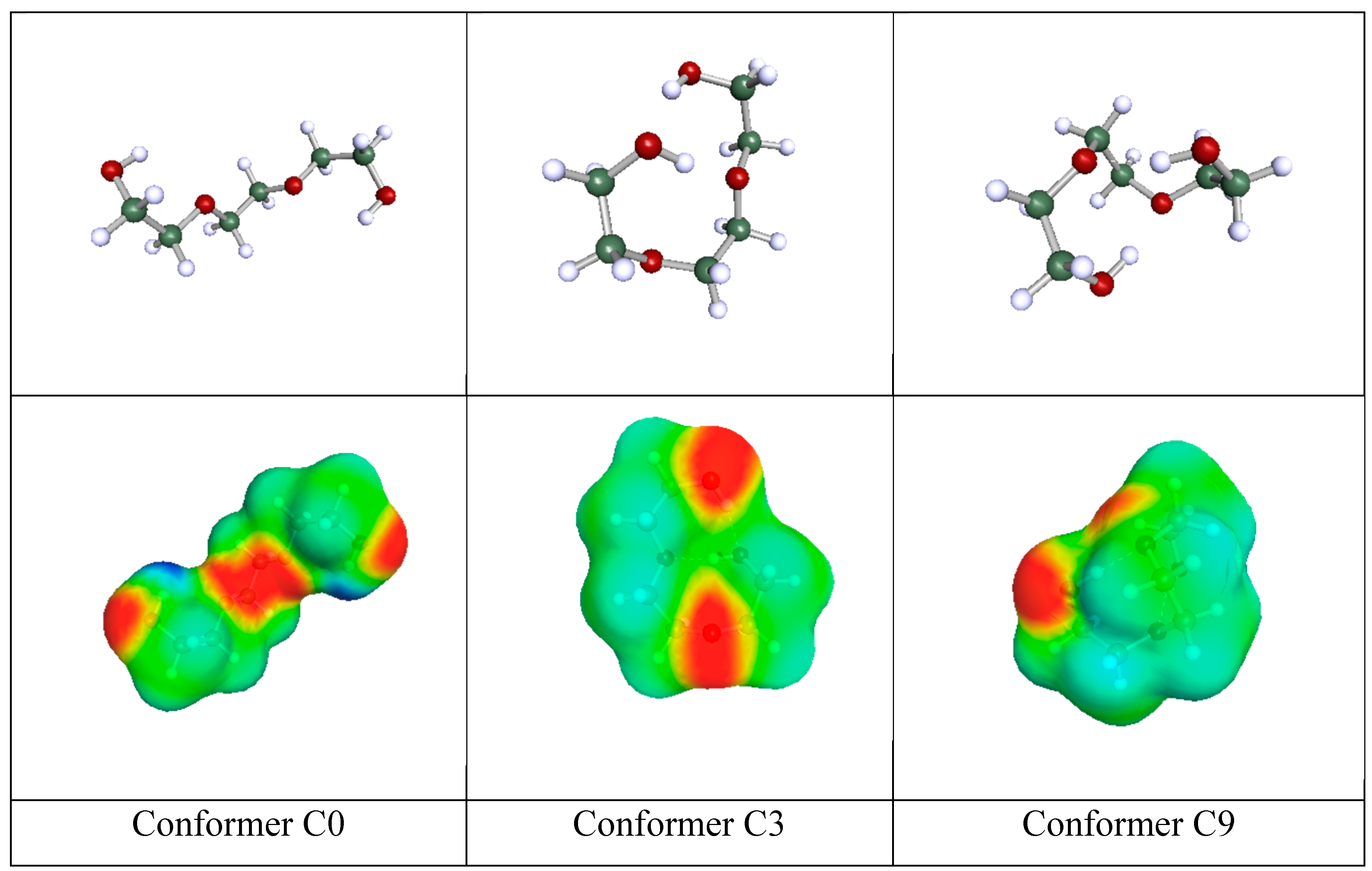

Table 1.
The hydrogen-bonding free-energy descriptors of common solutes.
* Ci refers to the i conformer of the solute [44].
Table 2.
The hydrogen-bonding contribution to solvation free-energy,(kJ/mol), of common aromatic solutes in 3 representative solvents using the augmented basicity descriptors βGB + 0.5 at 298.15 K.
Table 2.
The hydrogen-bonding contribution to solvation free-energy,(kJ/mol), of common aromatic solutes in 3 representative solvents using the augmented basicity descriptors βGB + 0.5 at 298.15 K.
Table 3.
Experimental [50] hydrogen-bonding (HB) solubility parameter, δhb, and predicted HB partial solvation parameter, σhb, of common compounds.at 298.15 K.
Table 3.
Experimental [50] hydrogen-bonding (HB) solubility parameter, δhb, and predicted HB partial solvation parameter, σhb, of common compounds.at 298.15 K.
| SOLUTE | kJ/mol | kJ/mol |  |
δhb [50] MPa0.5 |
 |
| METHANOL | 27.52 | 13.32 | 40.7 | 22.3 | 25.1 |
| ETHANOL | 25.07 | 12.13 | 58.5 | 19.4 | 19.8 |
| 1-PROPANOL | 24.76 | 11.98 | 75.2 | 17.4 | 17.4 |
| 1-BUTANOL | 24.96 | 12.08 | 91.5 | 15.8 | 15.8 |
| 1-PENTANOL | 24.86 | 12.03 | 108.6 | 13.9 | 14.5 |
| 1-HEXANOL | 25.06 | 12.13 | 124.9 | 12.5 | 13.6 |
| 1-HEPTANOL | 24.86 | 12.03 | 141.4 | 11.7 | 12.7 |
| 1-OCTANOL | 24.25 | 11.73 | 157.7 | 11.9 | 11.8 |
| 1-NONANOL | 24.76 | 11.98 | 174.4 | 10.6 | 11.4 |
| 1-DECANOL | 25.17 | 12.18 | 191.8 | 10.0 | 11.0 |
| 2-METHYL-1-PROPANOL | 22.07 | 10.68 | 92.8 | 15.9 | 14.6 |
| 2-METHYL-1-BUTANOL | 21.59 | 10.45 | 109.5 | 14.3 | 13.2 |
| 3-METHYL-1-BUTANOL | 24.55 | 11.88 | 109.3 | 13.3 | 14.3 |
| 2-ETHYL-1-HEXANOL | 21.31 | 10.31 | 156.6 | 11.8 | 11.0 |
| ISOPROPANOL | 25.16 | 12.10 | 76.9 | 16.4 | 17.3 |
| 2-METHYL-2-PROPANOL | 21.91 | 10.54 | 92.8 | 14.2 | 14.5 |
| 2-BUTANOL | 22.64 | 10.66 | 92.0 | 14.5 | 14.8 |
| 2-PENTANOL | 22.54 | 10.61 | 109.6 | 13.3 | 13.5 |
| 2-HEXANOL | 22.95 | 10.80 | 126.1 | 10.6 | 12.7 |
| 2-METHYL-2-BUTANOL | 19.95 | 9.39 | 109.6 | 13.3 | 12.5 |
| 4-METHYL-2-PENTANOL | 22.23 | 10.46 | 127.2 | 12.3 | 12.4 |
| CYCLOHEXANOL | 23.87 | 11.55 | 106.0 | 13.5 | 14.3 |
| 1-METHYLCYCLOHEXANOL | 17.87 | 8.04 | 123.4 | 12.5 | 10.9 |
| BENZYL ALCOHOL | 21.09 | 10.21 | 103.6 | 13.7 | 13.4 |
| PHENOL | 14.78 | 7.15 | 87.5 | 14.9 | 11.6 |
| o-CRESOL | 12.61 | 6.10 | 104.0 | 10.3 | 9.5 |
| m-CRESOL | 15.27 | 7.39 | 104.7 | 12.9 | 10.8 |
| p-CRESOL | 15.65 | 7.57 | 105.8 | 13.8 | 13.4 |
| p-ETHYLPHENOL | 8.56 | 4.14 | 118.6 | 12.8 | 6.90 |
| THYMOL | 10.64 | 5.15 | 166.9 | 10.8 | 6.7 |
| ACETIC ACID | 26.98 | 16.98 | 57.1 | 13.5 | 21.4 |
| PROPIONIC ACID | 25.54 | 16.08 | 75.0 | 12.4 | 18.1 |
| n-BUTYRIC ACID | 25.41 | 16.00 | 110.0 | 10.6 | 14.9 |
| n-PENTANOIC ACID | 25.27 | 15.90 | 109.2 | 10.3 | 14.9 |
| n-HEXANOIC ACID | 25.72 | 16.19 | 125.9 | 9.4 | 14.0 |
| ACRYLIC ACID | 25.43 | 16.00 | 68.5 | 14.9 | 18.9 |
| BENZOIC ACID | 21.91 | 13.79 | 100.0 | 9.8 | 14.4 |
| METHYLAMINE | 6.56 | 5.20 | 44.4 | 17.3 | 10.2 |
| ETHYLAMINE | 9.60 | 4.60 | 65.6 | 10.7 | 9.9 |
| n-PROPYLAMINE | 9.77 | 4.68 | 83.0 | 8.6 | 8.9 |
| ISOPROPYLAMINE | 8.67 | 4.16 | 86.8 | 6.6 | 8.1 |
| n-BUTYLAMINE | 9.47 | 4.54 | 99.0 | 8.0 | 8.0 |
| n-PENTYLAMINE | 9.52 | 4.56 | 116.1 | 7.2 | 7.4 |
| n-HEXYLAMINE | 9.59 | 4.59 | 133.0 | 6.5 | 7.0 |
| n-HEPTYLAMINE | 9.59 | 4.59 | 149.3 | 5.9 | 6.6 |
| n-OCTYLAMINE | 9.62 | 4.61 | 165.9 | 5.2 | 6.3 |
| DIMETHYLAMINE | 5.53 | 2.62 | 66.2 | 11.2 | 6.8 |
| DIETHYLAMINE | 3.33 | 1.58 | 103.2 | 6.1 | 4.0 |
| DI-n-PROPYLAMINE | 3.10 | 1.47 | 136.9 | 4.1 | 3.3 |
| ANILINE | 11.29 | 5.41 | 91.5 | 10.2 | 9.4 |
| FORMAMIDE | 20.69 | 23.05 | 39.8 | 19 | 22.7 |
| ACETAMIDE | 19.97 | 22.25 | 60.8 | 22.4 | 18.0 |
| N-METHYL FORMAMIDE | 10.69 | 11.91 | 59.1 | 15.9 | 12.9 |
| DIMETHYL SULFOXIDE | 2.16 | 0.93 | 71.3 | 10.2 | 3.7 |
| N,N-DIMETHYLFORMAMIDE | 0.00 | 0.00 | 77.0 | 11.3 | 0.0 |
| ACETONITRILE | 2.50 | 1.07 | 52.6 | 6.1 | 4.7 |
| PROPIONITRILE | 0.66 | 0.28 | 70.9 | 5.5 | 1.9 |
| ACRYLONITRILE | 2.61 | 1.12 | 67.1 | 6.8 | 4.2 |
| 2-METHOXYETHANOL c0 | 21.34 | 10.34 | 79.1 | 16.4 | 15.4 |
| 2-ETHOXYETHANOL solvent / solute | 17.53 | 8.50 | 97.8 | 14.3 | 12.2 |
| 2-ETHOXYETHANOL self-solv | 21.00 | 9.45 | 97.8 | 14.3 | 13.6 |
| 2-BUTOXYETHANOL | 18.51 | 8.97 | 131.6 | 12.3 | 10.9 |
| ETHYLENE GLYCOL solvent | 39.54 | 25.42 | 55.8 | 26 | 26.5 |
| ETHYLENE GLYCOL solute | 51.40 | 33.04 | 55.8 | 26 | 30.3 |
| 1,2-PROPYLENE GLYCOL solvent | 41.60 | 22.02 | 73.6 | 23.3 | 23.6 |
| 1,2-PROPYLENE GLYCOL solute | 56.49 | 29.90 | 73.6 | 23.3 | 27.7 |
| DIETHYLENE GLYCOLsolute | 59.58 | 26.81 | 94.9 | 20.7 | 25.0 |
| DIETHYLENE GLYCOL (self)solvent | 41.08 | 18.34 | 94.9 | 20.7 | 20.5 |
| DIPROPYLENE GLYCOL | 42.22 | 26.39 | 130.9 | 17.7 | 17.9 |
| TRIETHYLENE GLYCOL solute | 78.14 | 24.05 | 114.0 | 18.6 | 26.1 |
| TRIETHYLENE GLYCOL self-solvation | 40.07 | 8.11 | 114.0 | 18.6 | 17.0 |
| GLYCEROL | 83.77 | 38.67 | 73.3 | 29.3 | 33.8 |
| HYDROGEN PEROXIDE | 40.10 | 20.46 | 23.2 | 42.7 | 41.2 |
| WATER | 40.75 | 28.78 | 18.0 | 42.3 | 47.5 |
Disclaimer/Publisher’s Note: The statements, opinions and data contained in all publications are solely those of the individual author(s) and contributor(s) and not of MDPI and/or the editor(s). MDPI and/or the editor(s) disclaim responsibility for any injury to people or property resulting from any ideas, methods, instructions or products referred to in the content. |
© 2025 by the authors. Licensee MDPI, Basel, Switzerland. This article is an open access article distributed under the terms and conditions of the Creative Commons Attribution (CC BY) license (http://creativecommons.org/licenses/by/4.0/).
Copyright: This open access article is published under a Creative Commons CC BY 4.0 license, which permit the free download, distribution, and reuse, provided that the author and preprint are cited in any reuse.


