Modeling Charged Atoms for Atomistic Dynamics, using Equivariant GNNs

1. Quick Introduction to Pseudo-Vectors i.e Bra $\mathbf{\chi }$ and Ket $\mathbf{\chi }$ (Anti-Symmetric Inner Products), for GNN’s Equi-Variance Property

Quantum mechanics using Matrix, is called Matrix Mechanics, covered in great detail in almost all Quantum Mechanics text books such as Sakurai et al. [17]. We are only going to briefly cover, relevant multi-electron spherical tensor interactions occuring at quantum level, to implement/modify/experiment Equivariant GNNs, such as Allegro, Nequip, E3NN, which deploy geometric tensors, deploying convolution filters, filtering interactions by spherical harmonics [15,16].

In euclidean space dot products commute, i.e. $\mathbf{A}.\mathbf{B}=\mathbf{B}.\mathbf{A}$, however in quantum space represented as complex valued hilbert space $\mathcal{H}$, inner product $<A,B>=<B,A{>}^{*}$, where * indicates complex conjugate (just a mathematical trick to express inversion (reflection) across real axis), and A, B are complex vectors of n dimensions, this dot product can also be represented using hermitian matrix $\mathcal{H}$ (a complex extension of real valued symmetric matrix) as $\langle \mathcal{H}A,B\rangle =\langle A,{\overline{\mathcal{H}}}^{T}B\rangle =\langle A,\mathcal{H}B\rangle$ as $\mathcal{H}={\overline{\mathcal{H}}}^T$ i.e. complex square matrix $\mathcal{H}$ is equal to its conjugate $\overline{\mathcal{H}}$, transpose, producing real valued eigenvalues, representing position, momentum, spin, angular momentum or energy on a spectrum of Hermitian. Eigenvectors of Hermitian corresponds to quantum states associated with each measured value.

This dot product representation using complex conjugate of Hermitian, with elements of matrix in complex conjugate form (reflection across real axis), is also known as symmetric sesquilinear form (Hermitian form). We need to incorporate right orientation in order to get correct aggregation of angular momentum of various electrons in multi-body receptive field while using GNNs so that we can preserve equivariance, while performing aggregation of forces, momentums coming from various particles residing in given 3 D receptive field, characterized as sphere of given cutoff-radius.

In order to get better predictions about energy/forcefields triggering interatomic interactions, Density field Theory (DFT) approximates N electrons in a region as N-electron Hamiltonian, simplifying it later as Hohenberg-Kohn model of N electrons, using their spatial (x,y,z) co-ordinates, using Born-Oppenheimer approximation of total energy as sum of kinetic, rotaional, vibrartional and nuclear-spin energies as:

$$\widehat{H}\mathrm{\Psi }=\left[\widehat{Kinetic}+\widehat{Coulomb-Potential}+\widehat{elect.-elect.repul.energy}+\widehat{nuc-nucrepul.}\right]\mathrm{\Psi },$$

$$\widehat{H}=\sum _1^N-{\displaystyle \frac{{\hslash }^2}{2m}}{\nabla }_i^2+\sum _1^N{V}_{N{e}_{ionic}}\left(r_i\right)+V_{ee}(r_i,r_j)+V_{nn}(R_i,R_j)$$

under positive force of nuclei.

Kinetic energy ${\nabla }_i^2$ is invariant under rotation in x,y,z frame, Coulomb potentials ($V_{ne}$ are also invariant, assuming clamped nucleus Hamiltonian (nucleus becomes a fixed particle in classical mechanics sense), only hinderance towards implementing GNNs arises in modeling electron electron interactions ($V_{ee}$), as $V_{nn}$ can be ignored as nuclei are not getting so close in MD simulations unless material is approaching plasma state, if that is what we need to model, then we need to also add Yukawa potential ($V_{np}$ (proton, neutron interaction)), as we need to be aware of particles interacting...from Pauli’s exclusion principle, stating wavefunction must change sign when we switch order of Fermions (electron, protons etc.. we only care about electrons) involved:

$$\mathrm{\Psi }(f_1,f_2,,,f_n)=-\mathrm{\Psi }(f_1,f_2,...f_n),$$

where $f_1,f_2$ represents fermion’s (electron) position and spin. When Bosons are involved, we get

$$\mathrm{\Psi }(b_1,b_2,,,b_n)=\mathrm{\Psi }(b_1,b_2,...b_n).$$

A combined N particle wavefunction is thus represented using Slater determinants, as we can’t separate out contributions from each particle as separate wave function, due to spatial and spin component’s contributions on each particle’s spatial/spin terms:

$$|\mathrm{\Psi }(e_1,e_2,,,e_n)\rangle ={\displaystyle \frac{1}{\sqrt{N!}}}\left|\begin{array}{cccc}{\phi }_1\left(r_1\right)& {\phi }_2\left(r_1\right)& ...& {\phi }_N\left(r_n\right)\\ {\phi }_1\left(r_2\right)& {\phi }_2\left(r_2\right)& ...& {\phi }_N\left(r_n\right)\\ ⋮& \ddots & ...& ⋮\\ {\phi }_1\left(r_N\right)& {\phi }_2\left(r_N\right)& ...& {\phi }_N\left(r_N\right)\end{array}\right|$$

$$|\mathrm{\Psi }(e1,e2,,,en)\rangle ={\phi }_1\wedge {\phi }_2\wedge ...{\phi }_N$$

$$|\mathrm{\Psi }(e1,e2,,,en)\rangle =|{\phi }_1\rangle \langle {\phi }_2|\rangle \langle ...\langle |{\phi }_N$$

Bra (row vector) is multiplied to Ket (column vector) representing projection operator matrix showing projection of quantum state represented by Bra vector ${\phi }_2$ on quantum state represented by Ket vector ${\phi }_1$.

As one can see, last exterior product involving linearly independent ${\phi }_1,{\phi }_2...{\phi }_N$ equating to Slater determinant as bivectors (${\phi }_1\wedge {\phi }_2)$[19], a plane with directional rotation, operating on other vectors (${\phi }_3..{\phi }_N$) carrying, angular rotational information forward, at each step of exterior product computation. This exterior product, is also called Plucker embedding on Grassmannian manifold [4]. This brings us to reason for using GNNs, as GNNs map nodes to some embedding space by learning mapping functions.

This is all well and good but how will we compute this $V_{ee}$ value?

Here we need to bring separation of variables (spherical co-ordinates r, $\theta$, $\varphi$) and angular momentum’s projections on unit sphere (thus taming 3rd degree of freedom r as that can be linarly multiplied once we have potential energy surface value $V_{ee}$ for unit sphere as $r*V_{ee}$), into consideration. This projection is represented by a vector on the sphere’s surface. Vector’s length corresponds to the magnitude of the angular momentum projection along the axis defined by the vector’s direction. Direction of the vector indicates the specific axis on the sphere along which the angular momentum is projected. At Quantum scale, this projection is quantized, meaning it can only take on discrete values depending on the angular momentum quantum number (l) and its magnetic quantum number (m). In quantum mechanics, the z-component of angular momentum ($L_z$) is often used as the projection, and its possible values are quantized as $m\hslash$, where m is the magnetic quantum number ranging from -ℓ to +ℓ. We also have 2 spins, spin up and spin down.

This also explains why we will need to deploy tensors to accurately represent angular momentum of various electrons (adding individual orbital and angular momentum components) of multiple electrons interacting/orbiting around nucleus...

$$L_z=m\hslash =[-\ell ,+\ell ]\hslash$$

, where m is magnetic quantum number (describing spatial orientation of given orbital), ℓ angular momentum quantum number (describes shape of electron orbital, ℓ = 0 s orbital, ℓ = 1 p orbital, ℓ = 2 d orbital etc.. ℓ can take values from 0 to n-1, where n is principal quantum number (i.e. how far electron is from nucleus)), and L is total angular momentum vector, as we will also need direction of spin, component so that projection of angular momentum on z axis, are properly computed as electron states have to follow Pauli’s exclusion principle (i.e no two electrons in atom can have same values for n (distance from nucleus), ℓ shape of orbital, m spatial orientation and s spin [+1/2, -1/2]).

$$V_{ee}=J=\sum _{p=1}^N{L}_p+S_p\forall particlep\in sphereofreceptivefieldofcutoffradius=r$$

As we are modeling molecular dynamics, molecules are moving with time (translation) and these atoms are not fixed in structurally in space, molecules are rotating, inverting in 3D space. Even though we have x,y,z co-ordinates, we do not want to compute spherical versions using r, $\theta$, $\varphi$ at every instant to figure out translation, rotation and inversion status of each atom to compute what really has changed in terms of actual $V_{ee}$ or forcefield or momentum etc... with respect to, our point of reference of spherical receptive field.

This is where Lie Algebra (handling sequence of translation, rotation and inversion from hilbert space (allowing superposition of multiple basis states as linear combination to represent a quantum state using Linear Algebra terms such as eigenstates, infinte dimension to allow particle to move with time as dimension) $\mathcal{H}$ to ${\mathcal{R}}^3$ so that we can compare data with our LAMMPS values, use nearest-neighbors pairs etc.., representation theory (separating out similar representation of rotation as identical, i.e irrep) and special functions (spherical harmonics) come to rescue.

This can all only begin by understanding projection of group (Special Unitary group SU(2) on Special group of all rotations about origin SO(3).

Special here means that when we have matrix representation of mapping, determinant of the matrix is +1 (rotation) as -1 will represent reflection or loss of invariance for GNN and we will need to bring equivariance in to GNN. Groups can describe how individual actions (rotation, inversion, translation as time moves) taken together transform a molecule. Lie groups are mathematical tools representing continuous quantities as elements (i.e. there is no sudden breaks in rotational representation as molecule rotates etc..). These rotations, translation and inversion when done using irreducible representations (i.e. just like basis vectors, there is no subrepresentation for a given action exists), follow group laws of closure under addition etc. See general linear group of order 2 describing rotation matrix in 2D, using Euler’s identity $e^{i\theta }=cos\theta +isin\theta$ as :

$$GL(2,\mathcal{R})=SO(2,R)=\left(\begin{array}{cc}cos\theta & -sin\theta \\ sin\theta & cos\theta \end{array}\right)=e^{\theta \left(\begin{array}{cc}0& -1\\ 1& 0\end{array}\right)}=e^{\theta A}:detco{s}^2\theta -(-si{n}^2\theta )=1$$

Considering rotations in complex plane SO(2) is isomorphic to U(1):

$$GL(2,\mathcal{C})=SO(2,\mathcal{C})=U\left(1\right)=e^{i\theta }\leftrightarrow \left(\begin{array}{cc}cos\theta & -sin\theta \\ sin\theta & cos\theta \end{array}\right)$$

Using Shur’s lemma: if group is commutative then these irreducible representations are one dimensional, in Complex space $\mathcal{C}$ We know all imaginary terms cancel out as we do projections from Hilbert space to x,y,z i.e. $\mathcal{H}\to {\mathcal{R}}^3$ as at any time t, we will always have real valued position, potential energy, momentum terms. $\theta$ can be exchanged with time t, this $e^{tA}$ giving us full, time t dependent representaiton, of all rotations in 2 D space, as one matrix element.

Tangent space of Lie Groups (group representing rotations) at identity brings structures about multiplications, called Lie Algebra. These operations follow following rules (similar to cross product and Lie Bracket):

$$\begin{array}{cc}\hfill [i,i]& =0\forall i\in \mathfrak{g}\hfill \\ & =AB-BA\mathrm{A},\mathrm{B}\mathrm{are}\mathrm{Matrices}\mathrm{as}\mathrm{in}\mathrm{Matrix}\mathrm{Lie}\mathrm{group}\hfill \\ \hfill [i,[j,k\left]\right]+[j,[k,i\left]\right]+[k,[i,j\left]\right]& =0\forall i,j,k\in \mathfrak{g}\hfill \\ & =-[j,i]\hfill \end{array}$$

You can see now that

$$|\mathrm{\Psi }(e1,e2,,,en)\rangle ={\phi }_1\wedge {\phi }_2\wedge ...{\phi }_N={\phi }_1\otimes {\phi }_2\otimes ...{\phi }_N/({\phi }_1\square {\phi }_2\square ...{\phi }_N)$$

Where ${\phi }_1\square {\phi }_2\in {\phi }_1\otimes {\phi }_2$ is an ideal [24]. Since SU(2) and SO(3) both are Perfect Lee algebra (i.e. commutator: $[i,j]=i^{-1}{j}^{-1}ij$, a measure of commutativity, when taken for all elements producing derived algebra is equal to original algebra), we have ${\phi }_1\otimes {\phi }_1={\phi }_1\wedge {\phi }_1$[24] and $sign\left(\sigma \right){\phi }_1\otimes {\phi }_2={\phi }_1\wedge {\phi }_2$, i.e. $\wedge \mathrm{product}$ is anti-symmetric tensor product.

Modeling SO(3), Moving frame of reference, with time t, along with rotation along z axis:

$$x^{\prime }=A\left(\theta \right)x=\left(\begin{array}{ccc}cos\theta & -sin\theta & 0\\ sin\theta & cos\theta & 0\\ 0& 0& 1\end{array}\right)\left(\begin{array}{c}x\\ y\\ z\end{array}\right),y^{\prime }=A\left(\beta \right)y=\left(\begin{array}{ccc}cos\beta & 0& sin\beta \\ 0& 1& 0\\ -sin\beta & 0& cos\beta \end{array}\right)\left(\begin{array}{c}x\\ y\\ z\end{array}\right)$$

$$z^{\prime }=A\left(\gamma \right)z=\left(\begin{array}{ccc}cos\gamma & -sin\gamma & 0\\ sin\gamma & cos\gamma & 0\\ 0& 0& 1\end{array}\right)\left(\begin{array}{c}x\\ y\\ z\end{array}\right)$$

In ${\mathcal{R}}^3$, one can represent molecular dynamics by using translations, rotations along x,y,z and inversions with moving frame of reference as combinations of transformations such as for rotation we can combine above 3 transformations in successive order[18].

Changing x,y,z to spherical co-ordinates using unit sphere r=1, we get x= $1sin\theta cos\varphi$, y = $1.sin\theta sin\varphi$ and z = $1cos\theta$. Rotation group SO(3) will have no effect on r, thus we can represent a function $Y_l^m(\theta ,\varphi )$ which can represent any point, on unit sphere given parametrs $\theta$ and $\varphi$, this also means any rotation SO(3) can also be represented by $Y_l^m(\theta ,\varphi )$ as $Y_l^m(\theta ,\varphi )$ work as basis vectors for entire $L^2\left(S^2\right)$ Hilbert space. Solving laplacian ${\nabla }^{2}f(1,\theta ,\varphi )=0$, produces this well known solution [17] of $Y_l^m$ [25,26]. This shows how entire set of rotations, translations and inversions can be represented by spherical harmonics function parameterized by ℓ, m wrt to time t, by deploying consecutive translatios, rotations, inversions.

$$Y_{\ell }^m(\theta ,\varphi )=\underset{CondonShortlyPhase}{\underbrace{{(-1)}^m}}\underset{Constant}{\underbrace{{\mathcal{C}}_{\ell m}}}\underset{Phasefactor}{\underbrace{e^{im\varphi }}}\underset{AssociatedLegandrePolynomials}{\underbrace{P_{\ell }^{m}cos\theta }}$$

where:

$${\mathcal{C}}_{\ell m}=\sqrt{{\displaystyle \frac{(2\ell +1)}{4\pi }}{\displaystyle \frac{(\ell -m)!}{(\ell +m)!}}}\mathrm{where}\ell =0,1,2,..;m=-\ell ,\ell +1...\ell$$

This representation $Y_{\ell }^m$ is $(2\ell +1)$ dimensional irrep. (irreducible representation) of SO(3). Laplace-Beltrami operator ${\Delta }_s$ on $S^2$ in Hilbert space acts similar to Laplace operator in Euclidean space. This means Casimir operator $L^2$, not representing L square, just a symbol for angular momentum ∈$R^3$[25], for representation of SO(3) on unit sphere $\left(S^2\right)$ is the 2nd order differential operator of form[25]:

$$L^2=-\left({\displaystyle \frac{1}{sin\theta }}{\displaystyle \frac{\partial }{\partial \theta }}\left(sin\theta {\displaystyle \frac{\partial }{\partial \theta }}\right)+{\displaystyle \frac{1}{si{n}^2\theta }}{\displaystyle \frac{{\partial }^2}{{\partial }^2\varphi }}\right)=-\left({\Delta }_s\right)=\ell (\ell +1)I$$

Multi-particle interaction involving angular momentum:

Wigner-Eckart Theorm [10] states:

A tensor operator $T^k$ and two states of angular momenta ℓ and ${\ell }^{\prime }$ (for electron, spin is 1/2, which may align with orbital angular momentum I (s orbital, p orbital etc..) or not), there exists a constant (Clebsch Gordon coeff.) that for all (projections of angular momenta (ℓ,${\ell }^{\prime }$) along z axis), m,m’ and q, following holds:

$$\langle \ell m|T_q^{\left(k\right)}|{\ell }^{\prime }{m}^{\prime }\rangle =\underset{ClebschGordon}{\underbrace{\langle {\ell }^{\prime }{m}^{\prime }kq|\ell m\rangle }}\underset{ReducedMatrixElement}{\underbrace{\langle \ell \Vert T^{\left(k\right)}\Vert {\ell }^{\prime }\rangle }}$$

$${\left(T_{\ell m}\otimes T_{q,k}\right)}_{{\ell }^{\prime }{m}^{\prime }}=\sum _{m,q}\underset{Constanttimelookuptable}{\underbrace{{(-1)}^{-{\ell }^{\prime }+k-m^{\prime }}\sqrt{2.{\ell }^{\prime }+1}\left(\begin{array}{ccc}\ell & k& {\ell }^{\prime }\\ m& q& -m^{\prime }\end{array}\right)}}.\underset{independentofm,m^{\prime },q}{\underbrace{C_{\ell {\ell }^{\prime }}^k}}$$

Here $\left(\begin{array}{ccc}\ell & k& {\ell }^{\prime }\\ m& q& -m^{\prime }\end{array}\right)$ is not a matrix, this is called Wigner-3j [11] representation, showing interaction of angular momentum of electron in electron cloud of shape, ℓ, and its spatial location m, with another electron located in electron cloud of shape k, and spatial. 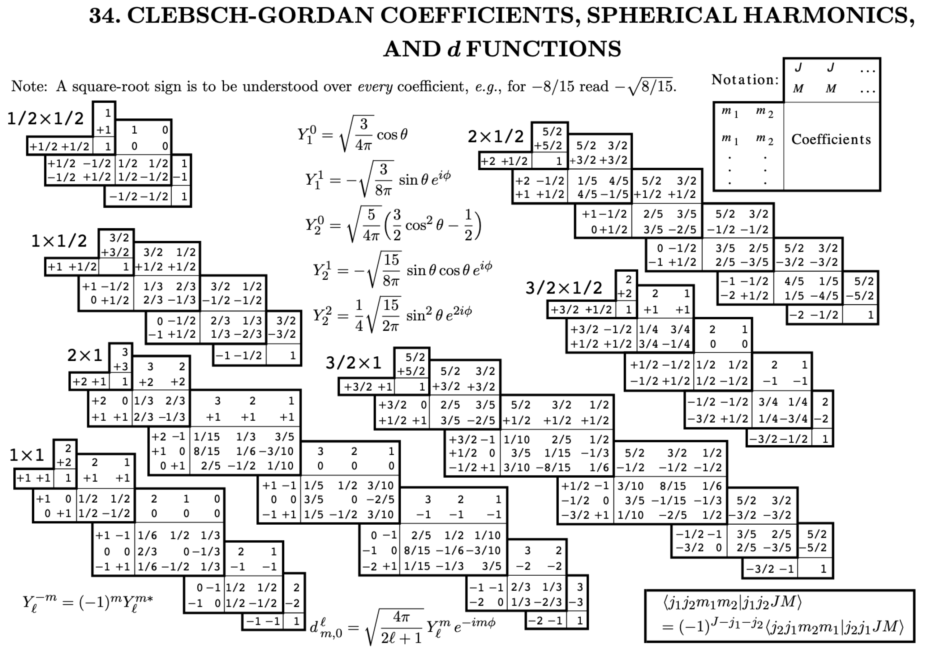location q, resulting in angular momentum (angular and spin) projected on to electron cloud of shape ${\ell }^{\prime }$ and location m’, as we sum these angular and spin part of angular momentum, separately. Clebsch-Gordon coefficients can be looked up from standard tables [12]. $C_{\ell {\ell }^{\prime }}^k$ needs to be computed only once for entire set of m,m’,q values ranging from $\{-\ell ,\ell \}$, $\{-{\ell }^{\prime },\ell \}$ and $\{-k,k\}$, saving us lot of repeated computation for multiple spatial locations represented by magnetic quantum numbers m,q,m’.

Figure 1. Clebsch Gordon Coefficients, Imgsrc : Particle Data Group K. Hagiwara et al.. [12]

Figure 1. Clebsch Gordon Coefficients, Imgsrc : Particle Data Group K. Hagiwara et al.. [12]

Representation of Rotation using Spherical Harmonics Basis

Here $T_q^{\left(k\right)}$ is spherical tensor operator, qth element rank k (k dimensional). Since we want to represent these molecule’s angular momentums in 3D space (${\mathcal{R}}^3$ or $\mathcal{H}=L^{(}{S}^2\left)\right)$), where atoms can be in any direction and moving, we need to have a single irrep representation, for various permutations [23] of rotations, inversions and translations filtering out equivalnet permutations (i.e. irrep., irreducible representation). This is direct in our case as Spherical Harmonics form a basis for irrep. of the rotation group, allowing us to liearly transform functions as combination of spherical harmonics bases $Y_{\ell }^m$.

This is where Wigner-d matrices [20]and d-functions come into picture..

Just like matrices of trignometric function in ${\mathcal{R}}^3$, are representing rotations around x,y,z axis (shown above), which can be combined to represent motion using Lie Algebra (SO(3) group) rules, spherical harmonics rotations, $\mathcal{R}(\alpha ,\beta ,\gamma )$ are governed by Wigner-D matrix [21], defined as:

$${\mathcal{D}}_{m{m}^{\prime }}^j(\alpha ,\beta ,\gamma )=\langle j{m}^{\prime }\left|\mathcal{R}(\alpha ,\beta ,\gamma )\right|jm\rangle =e^{-i{m}^{\prime }\alpha }{d}_{m{m}^{\prime }}^j\left(\beta \right)e^{-im\gamma }$$

where Wigner-(small)d-matrix is again defined as diagonal matrix, using basis as ${\mathcal{D}}_{m{m}^{\prime }}^j(\alpha ,0,0)=e^{-i{m}^{\prime }\alpha }{\delta }_{m{m}^{\prime }}$:

$$d_{m{m}^{\prime }}^j\left(\beta \right)=\langle j{m}^{\prime }|e^{-i\beta J_y}|jm\rangle ={\mathcal{D}}_{m{m}^{\prime }}^j(0,\beta ,0)$$

$$Y_{\ell }^m\left({\mathbf{r}}^{\prime }\right)=Y_{\ell }^m\left(r\right)e^{im\varphi }=\sum _{m^{\prime }=-\ell }^{\ell }[{\mathcal{D}}_{m{m}^{\prime }}^{(\ell )}{\left(\mathcal{R}\right]}^{*}{Y}_{\ell }^m\left(\mathbf{r}\right)$$

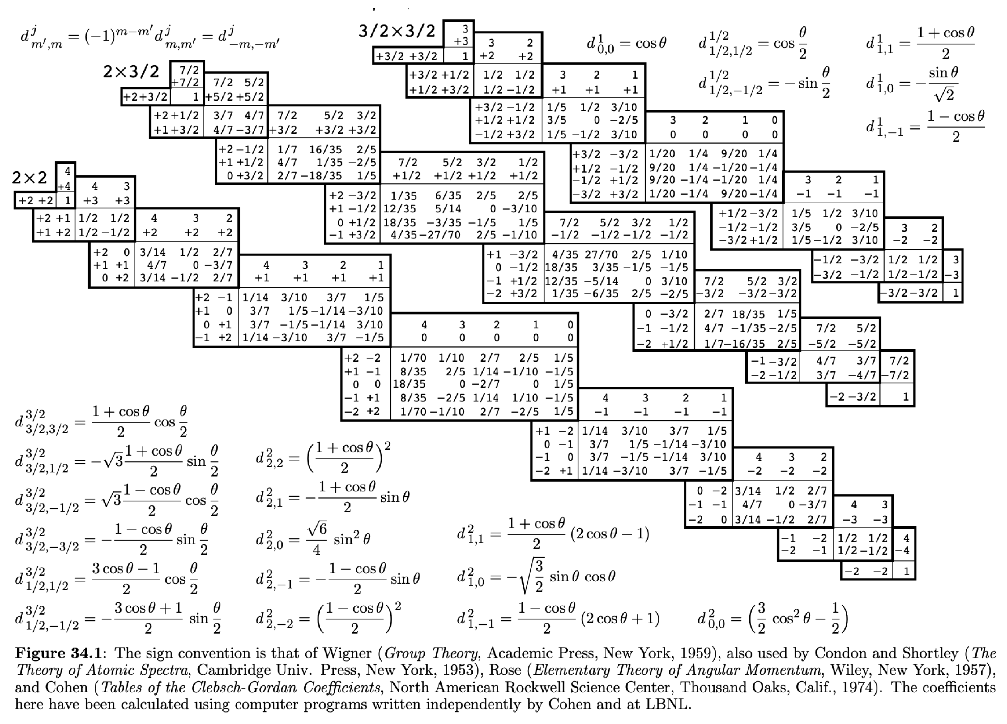
These Wigner-D matrices can also be combined like multiplication in Lie Algebra (matrix Lie Algebra SO(3) group), * above indicates that we should use complex-conjugate of an element from Wigner-D Matrix. Just like Clebsch Gordon coefficients table, we have table of d-Function at lower half of same page defined, requiring us to get these rotations by performing simple summation for $m{m}^{\prime }\in (-\ell ,to\ell )$ [12].

Figure 2. d-Functions to compute Wigner-d, Wigner-D, Imgsrc : Particle Data Group K. Hagiwara et al.. [12]

Figure 2. d-Functions to compute Wigner-d, Wigner-D, Imgsrc : Particle Data Group K. Hagiwara et al.. [12]

Samilarly inversion or parity is defined as[21], used in e3nn as :

$$Y_{\ell }^m(-\mathbf{r})={(-1)}^{\ell }{Y}_{\ell }^m\left(\mathbf{r}\right)$$

Co-ordinates conversion $L^2\left(S^2\right)\leftrightarrow {\mathcal{R}}^3$:

Conversion from $\mathcal{H}=L^2\left(S^2\right)$ space in $Y_{\ell }^m$ terms to $\mathcal{R}$ is not needed as $\theta$, $\varphi$ terms are the same. r term can be scaled, this was the reason for selecting a sphere of unit size. See Table of Spherical Harmonics below for few ℓ [22].

Figure 3. Spherical harmonics (Real part), Imgsrc : Wikipidea [22]

Figure 3. Spherical harmonics (Real part), Imgsrc : Wikipidea [22]

GNN - Equivariant Euclidean Neural Nets E3nn [14] came to represent Euclidean Neural Networks with spherical tensors to represent multi-particle interactions, preserving symmetry (including parity) in an equivariant way, using standard convolution neural nets (CNN) defined for r unit sphere as:

$$W\left(\overrightarrow{r}\right)=\underset{radial\leftarrow learnt,BesselFn,}{\underbrace{R\left(r\right)}}\underset{angularSphericalHarmonics}{\underbrace{Y_{\ell }^m}}\left(1\right)$$

Scalability of Density Function Theory, Hartree-Fock

For n electrons and N nuclei, using 3 spatial co-ordinates for each electron going into Shrodinger’s wave equation PDE, pinning nucleus as stationary, dimensional space for even small molecules such as Benzene (12 nuclei, 42 electron, each with x,y,z co-ordinates), grows at $n^{2}N={126}^2.36$ rate. We can ignore nuclei momentum as it rotates slower that electron, ignore cross-terms coming out of Shrodinger’s equations representing electron, nuclei interactions (not removing Coulomb potential altogether but keeping at as stationary value at some places) to further simplify... but still we end up with lot of variables. Modeling drug molecule efficacy in Cell’s protein rich environment, where drug molecule will interact with RNA, DNA molecules become prohibitively expensive.

Allegro - Learning Local Equivariant Representations [15]:

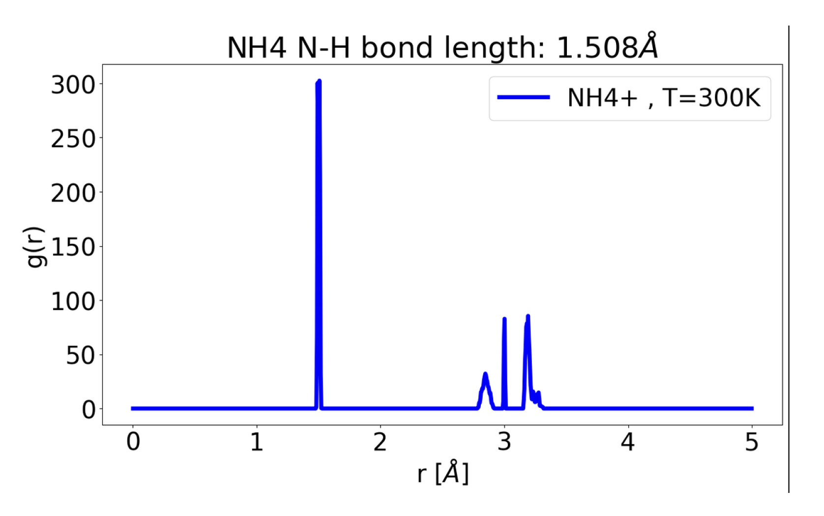
Any Message passing GNN, trying to model electron interactions, still needs to model potential energy surface (PES) at distance R of nuceli, assuming nuclear potential is average of nuclear-electron and inter-nuclear potentials so that GNN still predicts atomic-structure properties that are better than force-fields based methods, which ignore quantum level interactions and just compute forces among particles using x,y,z co-ordinates. This message passing increases exponentially with respect to cutoff radius, as we increase layers of our NN at each node (point cloud representation in our case). For 3 layer GNN and cut-off radius of 4 Angstrom (carrying 20 Ammonium ions), we will end up consolidating 4*3 = 12 Angstrom worth of space at each atom, carrying 533 ammonium ions. If strictly local scheme of Allegro is used, we will have $4^2$ = 16 times less aggregation, at each atom [15]. We preferred to build on top of Allegro for this reason, as we had limited compute resources (just 1 A100 GPU).

Our approach, SPICE Dataset[3] that has Charge, use dominant aggrgation locally: We gather messages but only allowed most dominant force to propogate for datasets such as SPICE, which has fore-fields and charge. Allegro uses SUM for aggregation which resulted in less than perfect predictions in our case where we limited training to only 100 epochs using SPICE dataset. Allegro team suggests 7 days of training using similar compute resource (A100 GPU) [15].

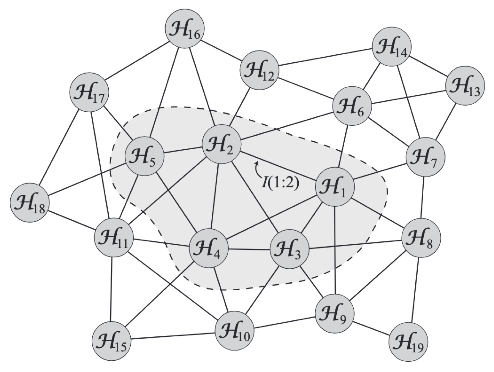
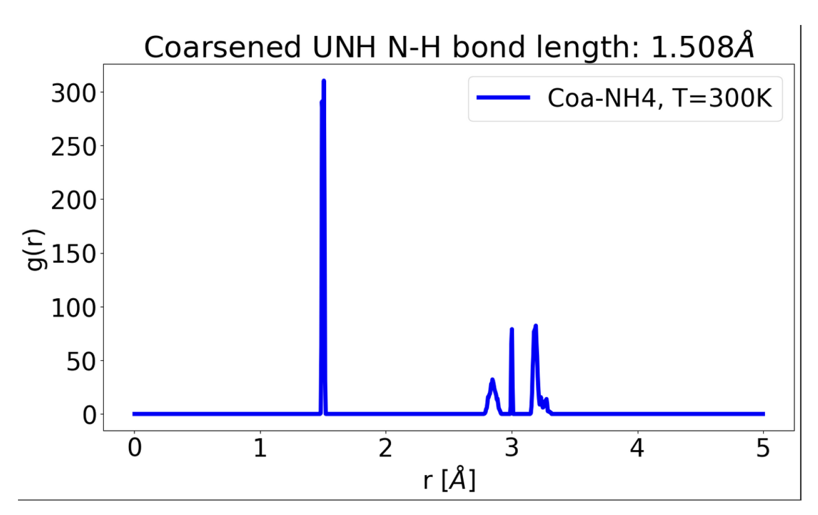
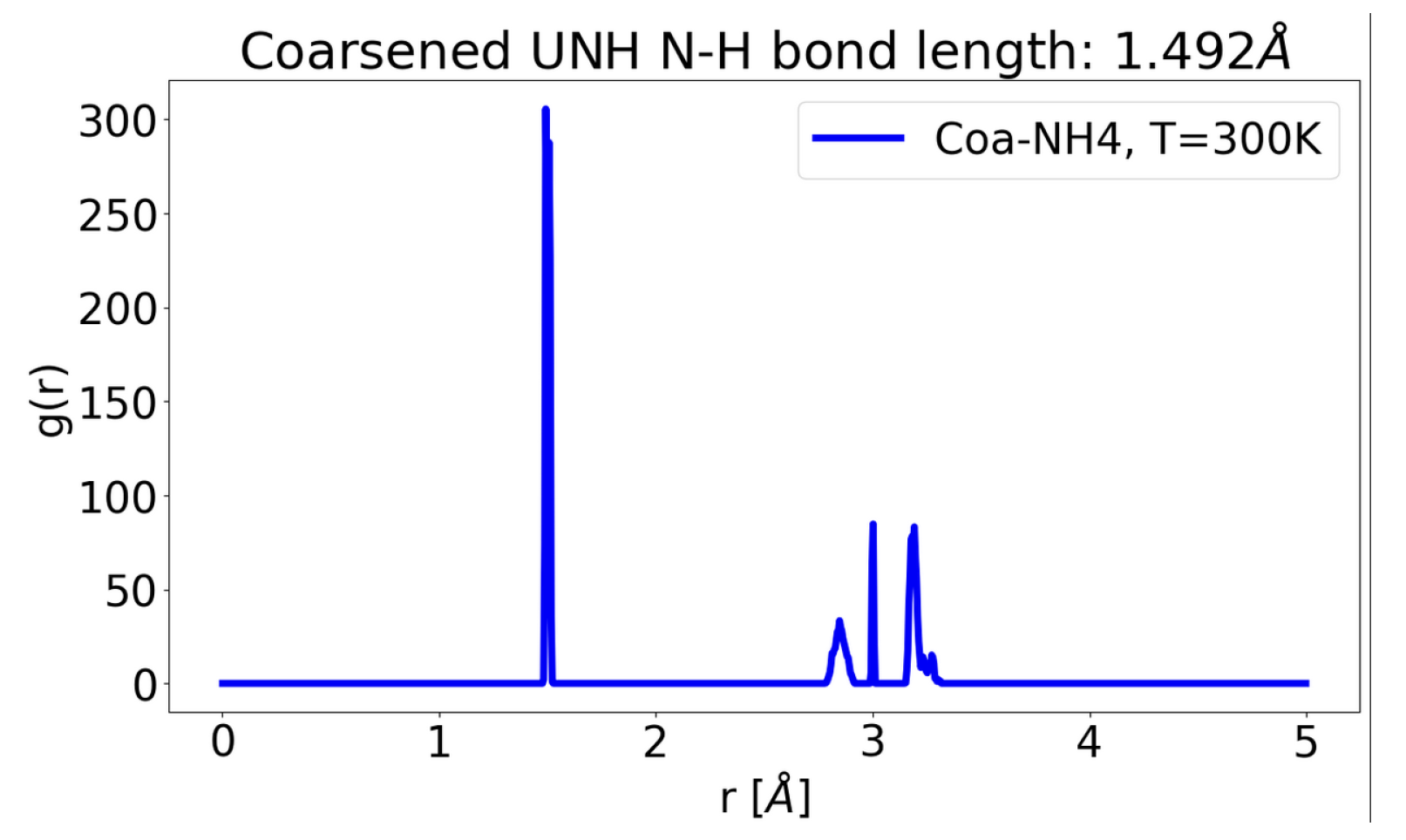
Finally, one can also construct a graph of Hilbert spaces [5] of regions (molecules interacting with other molecules), passing/summing information across nodes (used in Loop quantum gravity paper by ChunJun Cao et al.), which can be coarsened by cutting edges and approximating various nodes as one supernode passing back information to all previously cut edges, as it was happening before the cut, using ${⨂}_i^5{\mathcal{H}}_i={⨁}_i^5{\mathcal{H}}_i$ for shaded region below.

2. A Note About Data Augmentation to Facilitate Learning of Orientation

To capture correct orientation (translation, rotation and inversion invariance) of electron’s angular momentums, by just training GNNs using augmented datasets (as done for recognizing objects), requires 500 fold increase, just to handle rotations (not including inversions and/or shifts), in dataset. Kinetic energy and electron-electron interaction energy operators come as contant for systems of N electrons, only potential energy operator varies with time. This potential energy calculation is done using Tensor Field Network to sum of individual atomic potential energies, which is invariant to translation and equivariance to inversion and rotation [13], [14], thus saving us time to train neural networks with 500x data. For atoms of larger size such as 100,000 atom proteins, this learn by dataset approach becomes quickly unpractical as we need to have dataset where we do have an adequate representation of various angular momentums at each atom so that model can learn about how it can adequately direct molecule in a correct direction for reaction to take place [8].

Figure 4. Connected Hilbert Spaces as information graph, Imgsrc : Recovering Geometry from bulk entanglement by ChunJun Cao et al. [5]

Figure 4. Connected Hilbert Spaces as information graph, Imgsrc : Recovering Geometry from bulk entanglement by ChunJun Cao et al. [5]

3. Introduction

GNNs have been used to simulate fluid flow modeling navier-stokes equations. Here we summarize use of GNNs for molecular dynamics at quantum level, as solving multiparticle Shrodinger’s equations for N electrons is of complexity O($N^3$) or using Density Function Theory as O(N), which is still very high for systems modeling molecules of sizes 200,000+ atoms carrying millions of electrons. ([9]. We use SPICE [3] dataset that carries charge and force-field, to demonstrate that it is not best to use SUM as mode of AGGR., even when model is learning local equivariant representation as it is done in Allegro, based on e3nn/nequip [15], as force represented by charge dissipates across all atoms giving less optimal structural predictions. Using MAX, which preserves forces driven by charge, better; thus provides better predictions about structural properties (e.g. N-H bond length in Ammonium ion). We trained these models for 100 epochs, which took about 10 minutes. For better more accurate results, recommendation is to train these models for 7 days as Allegro team did for SPICE dataset. We can still confirm that results that we observed were in the right range. This framework can be applied to other compute intensive simulations where sets of nodes interact with each other as separate sets, by using receptive field based approach that defines the domain of interaction. This interactions could be interaction of a user across social networks to recommend products by using time-spent as receptive field, swarm of drones interacting in 3 D space by using spherical receptive field based on x,y,z co-ordinates (GPS data), or just using sets as nodes in Graph where collabarotive interactions needs to be modeled, as shown in connected Hilbert spaces in co-ordinate free loop quantum gravity approach.

The introduction should briefly place the study in a broad context and highlight why it is important. It should define the purpose of the work and its significance. The current state of the research field should be reviewed carefully and key publications cited. Please highlight controversial and diverging hypotheses when necessary. Finally, briefly mention the main aim of the work and highlight the principal conclusions. As far as possible, please keep the introduction comprehensible to scientists outside your particular field of research. Citing a journal paper [1]. Now citing a book reference [24,25] or other reference types [26,27]. Please use the command [28,29] for the following MDPI journals, which use author–date citation: Administrative Sciences, Arts, Behavioral Sciences, Businesses, Econometrics, Economies, Education Sciences, European Journal of Investigation in Health, Psychology and Education, Games, Genealogy, Histories, Humanities, Humans, IJFS, Journal of Intelligence, Journalism and Media, JRFM, Languages, Laws, Literature, Psychology International, Publications, Religions, Risks, Social Sciences, Tourism and Hospitality, Youth.

4. Materials and Methods

Interaction between various sets of points representing atoms of different molecules can be represented by using a sphere in 3 D space, carving out points of interests, as we capture interaction among electron clouds. This is defined by supplying cutoff radius parameter as shown below [27], [1]. Picture shows a small planar molecule in orange plane with red dots representing its atoms, interacting with molecule with atoms dispersed in larger 3D space represented by blue dots as its atoms. Bonds among these atoms are shown as red and blue edges for each molecule respectively.

In order to capture multi molecule interactions, we first pre-process dataset to produce extxyz formatted molecules. Extended xyz format keeps forcefileds and charge information available at each atom. SPICE dataset is in hdf5 format so we can extract this extended xyz information for each class of molecules as needed. We then move a sphere of preset cutoff radius from atom to atom, capturing available atoms at given point and their respective charge and force-fields. This was we are not only creating a new NN at each point but also a new graph at each point (atom), based on molecular dynamical interactions happening at various nodes of each molecule at desired temperature.

Following fig 2 shows two such points P, $P^{\prime }$ with green sphere. Choosing the correct cutoff radius is thus of paramount importance to achieve success using GNNs. As if sphere is too small we will not adequately capture interatomic quantum level interactions, so our model will behave like a model based solely on forcefields. Choosing a sphere of large size will show that quantum-level interactions have no effect since many of these forces are inversely proportional to $r^2$, thus completely missing impact of electron clouds on molecular dynamics, as these forces are only applicable at short distances (femto-meter to few angstroms). For SPICE data set, the recommended cutoff distance is 4.2 angstroms.

This methodology QM/MM (Quantum Mechanics and Molecular Mechanics) using GNNs accelerates modeling significantly as we are not longer solving multiparticle time-dependent Shrodinger’s partial differential equations but are only figuring out non-linear Plucker embedding representations on Grassmannian [4] manifolds using GNN. We can also simulate breaking/forming of bonds as needed as we only concern ourselves at given reseptive field (green sphere) at a time. If there are enough forces/charge present we can remove edge or form an edge between nodes of two separate molecualr graphs. SPICE dataset [3] does not yet have, atomic bonds breakage/formation information, however another dataset Transition-1x does... [2]

We do not perform any searches to get node lists of interest at any given node as we pre-process this data in form of verlet lists, named after Loup Verlet, using LAMMPS (Large-scale Atomic/Molecular Massively Parallel Simulator) with complexity O($N^{1.666}$), Cell lists option can further reduce this complexity to O(N). [6,7].

Figure 5. Protein Ligand Interaction Source: Cell - How aberrant N-glycosylation can alter protein functionality and ligand binding: An atomistic view, Matteo Castelli et. al.

Figure 5. Protein Ligand Interaction Source: Cell - How aberrant N-glycosylation can alter protein functionality and ligand binding: An atomistic view, Matteo Castelli et. al.

We share our colab notebook, and instructions to generate extxyz data that can help generate other molecule sets from SPICE dataset.

5. Data Pipeline

ASE libraries can map SPICE hdf5 data into extended xyz (called .extxyz by vputz) format. We have all scripts shared at our github repo [27].

Table 1. extxyz.py list-subsets.

Index	Subset Molecules	Version
1	SPICE DES Monomers Single Points Dataset	v1.1
2	SPICE DES370K Single Points Dataset Supplement	v1.0
3	SPICE DES370K Single Points Dataset	v1.0
4	SPICE Dipeptides Single Points Dataset	v1.2
5	SPICE Ion Pairs Single Points Dataset	v1.1
6	SPICE PubChem Set 1 Single Points Dataset	v1.2
7	SPICE PubChem Set 2 Single Points Dataset	v1.2
8	SPICE PubChem Set 3 Single Points Dataset	v1.2
9	SPICE PubChem Set 4 Single Points Dataset	v1.2
10	SPICE PubChem Set 5 Single Points Dataset	v1.2
11	SPICE PubChem Set 6 Single Points Dataset	v1.2
12	SPICE Solvated Amino Acids Single Points Dataset	v1.1 1

¹ From SPICE 2.0.1 hdf5 dataset.

Table 1. extxyz.py list-subsets.

Index	Subset Molecules	Version
1	SPICE DES Monomers Single Points Dataset	v1.1
2	SPICE DES370K Single Points Dataset Supplement	v1.0
3	SPICE DES370K Single Points Dataset	v1.0
4	SPICE Dipeptides Single Points Dataset	v1.2
5	SPICE Ion Pairs Single Points Dataset	v1.1
6	SPICE PubChem Set 1 Single Points Dataset	v1.2
7	SPICE PubChem Set 2 Single Points Dataset	v1.2
8	SPICE PubChem Set 3 Single Points Dataset	v1.2
9	SPICE PubChem Set 4 Single Points Dataset	v1.2
10	SPICE PubChem Set 5 Single Points Dataset	v1.2
11	SPICE PubChem Set 6 Single Points Dataset	v1.2
12	SPICE Solvated Amino Acids Single Points Dataset	v1.1 1

¹ From SPICE 2.0.1 hdf5 dataset.

We can look at various keys using :

python extxyz.py subset 1 –out test then print hf.keys() to get conformer/molecule.

We can then extract extended xyz co-ordinates for say Argenine in 0D1 conformation by:

python extxyz.py group ’0D1 ARG’ –out gtest

We can follow these steps to get data pertaining to any desired group, see SPICE Dataset documentation. [28].

My Google Colab notebook NH4_CoaSpPyDG.ipynb, also shared [29], uses, DES.

6. Code

See "Graph Sparsification by Edge reduction" section of NH4_CoaSpPyDG.ipynb for allegro.nn modifications. Allegro folds edgewise energies into nodes using "sum", we changed this to max for charged particles such as Ammonium Ion.

7. Results

N-H Bond length in Ammonium Ion

As per Open-AI [30]: The number of ammonium ions ($N{H}_4^{+}$) in a sphere with a radius of 12 angstroms depends on the density of the ions in the sphere.

Explanation : The ionic radius of an ammonium ion is 1.48 angstroms (Å). The atomic radius of an isolated neutral atom is usually between 0.3 and 3 angstroms...

7.1. Unmodified Allegro

Figure 6. Default run of Allegro - N-H Bond Length Prediction

Figure 6. Default run of Allegro - N-H Bond Length Prediction

7.2. Coarsened Allegro (33 Percent Noise, Using Sum

Figure 7. Coarsened Allegro - N-H Bond Length Prediction

Figure 7. Coarsened Allegro - N-H Bond Length Prediction

7.3. Coarsened Allegro with 33 Percent Noise Using Max

Figure 8. Coarsened Allegro using max for charge - N-H Bond Length Prediction

Figure 8. Coarsened Allegro using max for charge - N-H Bond Length Prediction

8. Discussion

As we can observe, max mode of message aggregation in presence of charge, in Ammonium ion has least amount of N-H bond lenfgth prediction error, even when model was trained for 100 epochs in all cases. Adding perturbations and noise did not change anything. We decided to add noise as first order approximation for clustering of dense electron clouds to further accelerate Machine Learning Interatomic Potentials as used in ACE (Atomic Cluster Expansion) representing aromic densities. We are exploring edge collapsing, merging dense cluster to super nodes as first pass to further allow large model (500,000 atoms or more) MD simulations on single A100 GPUs. This will enable quick discoveries of macro structural , energy features of large set of atoms.

9. Conclusions

Coarsening of atomic clusters using ML or data pre-processing can enable very large scale Molecular Dynamics runs allowing researchers to explore hierarchical, long range atomic clusters interactions at low cost. This may allow material scientist to explore environmental impact of stress exposure to material strength, or model other slowly cumulative effects of temperature, pressure, exposure to corrosive envirnments over long term. This study is first step towards that goal.

References

1. Matteo Castelli-1, Pengrong Yan-2, Anna Rodina-2, Chander S. Digwal-2, Palak Panchal-2, Gabriela Chiosis-2,3, Elisabetta Moroni-4, Giorgio Colombo, T. How aberrant N-glycosylation can alter protein functionality and ligand binding: An atomistic view. Cell 2023, 31.8, 987–1004.
2. Matthias Shreiner-1, Arghya Bhowmik, Tejs Vegge, Jonas Busk, Ole Winther T. Transition1x - a dataset for building generalizable reactive machine learning potentials. Nature 2022, 9.779.
3. Eastman, P. , Behara, P.K., Dotson, D.L. et al. T. SPICE, A Dataset of Drug-like Molecules and Peptides for Training Machine Learning Potentials. Sci Data 10, 11 (2023) Nature 2022, 9.779. [CrossRef]
4. Aoto, Yuri Alexandre and da Silva, Márcio Fabiano T. Calculating the distance from an electronic wave function to the manifold of Slater determinants through the geometry of Grassmannians. Phys. Rev. A 102, 5, (2020). Physical review A 2020, 102.052803. [CrossRef]
5. ChunJun Cao, Sean M. Carroll, Spyridon Michalakis. T. Space from Hilbert Space: Recovering Geometry from Bulk Entanglement. Arxiv 2016. [CrossRef]
6. A. P. Thompson, H. M. Aktulga, R. Berger, D. S. Bolintineanu, W. M. Brown, P. S. Crozier, P. J. in ’t Veld, A. Kohlmeyer, S. G. Moore, T. D. Nguyen, R. Shan, M. J. Stevens, J. Tranchida, C. Trott, S. J. Plimpton, T. LAMMPS - a flexible simulation tool for particle-based materials modeling at the atomic, meso, and continuum scales. Comp Phys Comm, 271 (2022) Comp Phys 2022, 10817. [CrossRef]
7. Kun Li · Shigang Li · Shan Huang · Yifeng Chen · Yunquan Zhang, T. FastNBL: fast neighbor lists establishment for molecular dynamics simulation based on bitwise operations. The Journal of Supercomputing (2019) J Super Computing 2019 75:8339–8340. [CrossRef]
8. Workshop on Equivariant Networks. Available online: https://sites.google.com/view/equiv-data-aug/home (13-01-2025).
9. Dutch-Flemish Scientific Computing Society Woudschoten Conferences. Available online: https://wsc.project.cwi.nl/woudschoten-conferences/2008-woudschoten-conference/Mohlenkamp_2_lezing.pdf 2008 (14-01-25).
10. Wigner-Eckart Theorem. Available online : https://en.wikipedia.org/wiki/Wigner.
11. Wigner-J Matrix. Online : https://en.wikipedia.org/wiki/3-j_symbol (18-Jan-25).
12. Clebsch Gordon Coefficients Table . Online : https://pdg.lbl.gov/2002/clebrpp.pdf (18-Jan-25).
13. Thomas, N. Thomas, N. et al. T. Tensor field networks: Rotation-and translation-equivariant neural networks for 3d point clouds. arXiv preprint arXiv:1802.08219 (2018). https://arxiv.org/pdf/1802.08219 Arxiv 2018 1802.08219v3.
14. Mario Geiger and Tess Smidt, T. e3nn: Euclidean Neural Networks. https://arxiv.org/pdf/2207.09453. Arxiv 2021 2207.09453.
15. Albert Musaelian, Simon Batzner et al. T. Learning Local Equivalent Representations For Larg-Scale Atomistics Dynamcis. Arxiv 2022 2204.05249. [CrossRef]
16. Chaitanya K. Joshi, Taco Cohen et. al. T. On the Expressive Power of Geometric Graph Neural Networks. Arxiv 2023 2301.09308. [CrossRef]
17. J. J. Sakurai, Jim Napolitano T. Modern Quantum Mechanics. Cambridge 2017 ISBN-1108422411.
18. Shu Hotta T. Mathematical Physical Chemistry. Springer 2023 ISBN-978-981-99-2512-4.
19. Bivector-Wikipedia. Available online: https://en.wikipedia.org/wiki/Bivector (12-15-2025).
20. Wigner-D Matrix. Available online: https://en.wikipedia.org/wiki/Wigner_D-matrix (12-18-2025).
21. Spherical harmonics Rotations. Available online: https://en.wikipedia.org/wiki/Spherical_harmonics#Rotations (12-18-2025).
22. Table of Spherical harmonics. Available online: https://en.wikipedia.org/wiki/Table_of_spherical_harmonics (12-18-2025).
23. Willard Miller, Jr.; Lie Theory and Special Functions, Volume 43; Elsevier: Paperback ISBN: 9780124110472 pp 262-266 1968.
24. Graham J. Ellis; A non-abelian tensor product of Lie algebras; Volume 33, Glasgow Mathematical Journal: Issue 1 pp. 101 - 120 1991.
25. Peter Woit; Quantum Theory, Groups and Representations; Springer: Issue 1 pp. 115 - 120 2017.
26. Peter Woit; The Spherical Harmonics; Santa Cruz Institute for Particle Physics, Physics116: http://scipp.ucsc.edu/ haber/ph116C/SphericalHarmonics_12.pdf 17-01-2025.
27. GIT Repository carrying extxyz.py to extract extxyz data for modified Allegro. Available online: https://github.com/v365747/GraphCoarseningGNN (12-18-2025).
28. SPICE Dataset creation scripts GIT Repository. Available online: https://github.com/openmm/spice-dataset (12-18-2025).
29. NH4_CoaSpPyDG.ipynb Modified Allegro predicting N-H Bond length in Ammonium Ion. Available online: https://colab.research.google.com/drive/1PRkvlrWmj3TAktqGIZ4DJkVYEHse0tex (12-18-2025).
30. OpenAI. (2023). ChatGPT (Mar 14 version) [Large language model]. Available online : https://chat.openai.com/chat (12-18-2025).
Disclaimer/Publisher’s Note: The statements, opinions and data contained in all publications are solely those of the individual author(s) and contributor(s) and not of MDPI and/or the editor(s). MDPI and/or the editor(s) disclaim responsibility for any injury to people or property resulting from any ideas, methods, instructions or products referred to in the content.
Copyright: This open access article is published under a Creative Commons CC BY 4.0 license, which permit the free download, distribution, and reuse, provided that the author and preprint are cited in any reuse.
Prerpints.org logo
Preprints.org is a free preprint server supported by MDPI in Basel, Switzerland.
Subscribe
Disclaimer
Terms of Use
Privacy Policy
Privacy Settings
© 2025 MDPI (Basel, Switzerland) unless otherwise stated