
Submitted:
20 January 2025
Posted:
21 January 2025
You are already at the latest version
Abstract
This paper deals with the analysis of vibrations induced by a moving bogie passing through a single-layer model of a railway track. The emphasis is placed on the possibility of unstable behavior in the subcritical velocity range. All results are presented in dimensionless form to cover a wide range of possible scenarios. The results are obtained semi-analytically, however the only “numerical” step is related to solving the roots of polynomial expressions. No numerical integration is used, and therefore even completely undamped scenarios can be easily solved, as damping is not necessary for numerical stability. The vibration shapes are presented in the time domain in closed form. It is concluded that increased foundation damping aggravates the situation, but in general the danger of instability in the subcritical velocity range of moving bogie is less than two moving masses, especially for higher mass moments of inertia of the bogie bar and primary suspension damping. It is also tested how the obtained results were changed by considering a Timoshenko-Rayleigh beam instead of Euler-Bernoulli. Although some cases may seem academic, it has been shown that instability in the supercritical velocity range cannot be assumed as guaranteed.
Keywords:
contour integration
; integral transforms
; critical velocity
; instability
; transient vibrations
; analytical solution
1. Introduction
One of the effective ways to combat climate change and reduce the carbon footprint is to prioritize rail over road transport. This naturally implies the need to increase the railway network capacity by increasing travel speed, number of trains and axle loads. Such increased demands emphasize the need of ensuring the passenger safety and comfort. The upper limit for the travel speed is usually derived from the value of the critical velocity, which in this context corresponds to the critical velocity of the moving force, which is equal to the lowest velocity of wave propagation in the supporting structure, resulting from the dynamic interaction of all the parts involved and can be called the critical velocity for resonance.
Another commonly used indicator for ensuring the safety of train passage is the receptance curve, which, however, only indicates the natural frequencies of the supporting structure. The frequencies that cause unstable behavior cannot be identified using the receptance curves because they depend on the mass and velocity of the moving object. Therefore, it is necessary to study the transient vibrations caused by the moving vehicle and the associated so-called induced frequencies, which can identify whether the motion will be stable or unstable. Nevertheless, the problem of instability was somehow overlooked because it was shown that a single moving mass or oscillator can achieve unstable behavior only in the supercritical velocity range, and since this region is a priori excluded from the design of the track, the issue of instability was not found to be crucial.
However, the dynamic interaction of two moving proximate masses can lead to a different situation, which surprisingly worsens with increased foundation damping. Such cases have already been identified in the author’s previous works.
Moving load problems are still very active scientific topics related to transportation engineering applied to rail or road transport. Several simplifications have been introduced to solve these problems more efficiently and to present the results in a more compact form suitable for optimization and sensitivity analyses. The simplifications are applied to the supporting structure or to the moving vehicle, or both, depending on the problem being solved. In addition to the analysis of the influence of several parameters on dynamic performance, topics of particular interest are critical velocity for resonance, critical frequency for resonance, instability and dynamic interaction of proximate inertial objects.
Typical simplifications at the level of supporting structure led to layered models consisting of beams, point masses and spring-damper elements. These models are quite popular for their simplicity and computational efficiency. Such simplified models, together with simplified vehicle models, are used in more practical studies as well as in some more theoretical studies. The applicability of the three-layer model in railway applications is analyzed in [1] and an overview of some features of the one-, two- and three-layer models is given in [2].
Many research works have been developed during the last decades; thus, this review will essentially focus on the most recent publications.
In [3] a critical discussion of developments in the field of dynamic response of rigid road pavements to a moving vehicle is presented. Rigid pavements consist of an elastic concrete plate or jointed plates resting on a supporting foundation. Such models are also used in railway engineering, only with different parameters. The supporting medium can be modeled as a system of spring-damper elements or as a homogeneous or layered half-plane/space with infinite or finite depth. The paper summarizes the works where the material behavior of the subgrade layers is isotropic as well as anisotropic, viscoelastic, poroelastic or inelastic. In [4] another more detailed review by the same authors on both types of pavements, i.e. rigid and flexible, is given. In these works, vehicles are simulated by constant concentrated or distributed over a finite line/area moving forces, while their inertial effect and thus the possibility of instability is omitted. In [5], the plane strain model is used in the moving mass problem to analyze instability issues.
In [6], although also focused on road pavements, the guiding structure model corresponds to the one-layer model, which is often used in railway applications. The model is crossed by a two-mass oscillator with a contact spring-damper element, also very common in railway applications. The harmonic roughness of the roadway is taken into account, but no instability or critical velocity are analyzed. Since there is only one contact point, the dynamic interaction of proximate objects cannot be observed. The work focuses on the analysis of the effect of the nonlinearity of the foundation, which is addressed by the Adomian decomposition method. Moving coordinates are implemented and the results are limited to the steady-state part of the response, since only a single Fourier transform is applied. Such an approach in fact removes the inertial effects of the moving object. The research findings are that there is a critical value for the nonlinear stiffness, which increases with the vehicle velocity and the foundation damping.
As for the railway applications, the nonlinearity of the supporting structure is analyzed in [7]. A two-layer model is implemented, and a simplified vehicle model is used. A new nonlinear stiffness model that comprehensively characterizes the ballast properties by a displacement-dependent stiffness, frequency-dependent stiffness, hysteresis, and time/space-varying features is developed. The model is validated by experimental measurements processing the ground penetrating radar signal using the adaptive optimal kernel time–frequency representation method.
Moving force problems are simpler than moving mass problems, especially for finite length supporting structures, for which analytical solutions exist and can be formalized by modal expansion. However, a relatively recent study [8] still analyzes this problem for a double-beam structure focusing on the effect of various boundary conditions. Modal expansion is efficient on finite structures, and although the motion of mass on finite Euler-Bernoulli beams without elastic foundation and damping is a classic problem that has already been addressed by several researchers, there are still new results and physical insights worth publishing for such a simple structure as shown in [9]. Moreover, in [10] a new equivalent lumped parameter model is proposed to describe the vibrations of simply supported beams without an elastic foundation under the action of a moving force, which is a classic problem with a fully analytical solution. In [11], vibrations of a similar structure subjected to a moving mass are solved using Green’s function method, with the aim to analyze the effect of boundary conditions, mass velocity and its ratio with respect to the beam mass.
More practical studies usually deal with typical degradation on railway lines, that is transition zones, rail corrugation, maintenance optimization or possible failures. For example, in [12] the effect of temperature on concrete cracking in unballasted lines is analyzed; in [13] failure of suspension damper in railway vehicles based on the cross-correlation analysis of bogie accelerations is presented.
Regarding the transition zones, it is known that the sudden change in the vertical stiffness of railway tracks increases the dynamic loads and causes numerous defects on ballasted tracks. The main geometric parameters of the approach slab for short-span bridges are optimized in [14]. A finite element model is built and subjected to a series of moving forces. The model was validated with field measurements acquired using a laser/camera-based measuring technique. The obtained geometric sensitivity analysis results show that the rail and ballast displacements can be significantly reduced by using a geometrically optimized approach slab along the transition zone of a railway bridge.
In [15], a revolutionary new design recently proposed to mitigate the negative effects of transition zones is evaluated for extreme conditions. This new design of a transition structure is called SHIELD (Safe Hull Inspired Energy Limiting Design), and was designed to reverse the propagating waves by inverting the shape of the embankment zone, thus directing the wave energy towards the foundation instead of upwards to damage the railroad. It was found that the novel design effectively mitigates dynamic amplifications and leads to a smooth distribution of deformation energy across subcritical, critical and supercritical velocity regimes in both directions of travel, meaning that the expected traffic-induced degradation will be as uniform as possible in the longitudinal direction.
Transition zones are directly linked to the floating sleeper phenomenon, for which a novel approach in modelling is presented in [16], providing an accurate mathematical model with a minimum number of degrees of freedom supported by extensive field measurements of a railway track. Although the observed phenomenon is very complex, a simplified mathematical model of one degree of freedom has proven to be sufficiently accurate for its characterization.
Regarding rail corrugation, a new hypothesis for the formation process of short pitch rail corrugation is presented in [17]. A dynamic finite element (FE) wheel-track model is used to verify the hypothesis by reproducing corrugation initiation and its consistent growth. The FE model is composed of discrete elements as in other works with semianalytical or analytical solutions. The supporting structure is in fact equivalent to a two-layer model extended to 3D, and both the railpads and the foundation, which in fact only corresponds to the ballast layer, are modeled by a set of spring-damper elements acting in three directions. The wheelset and rails are modeled in detail using 3D elements, and then the remaining mass of the vehicle is lumped and placed above the primary suspension. It is found that longitudinal compression modes are responsible for corrugation initiation. The proposed mechanism can explain field observations. In [18] the finite element model is validated using a downscale V-Track test rig.
Transition zones are related to transition radiation. In this context it is worthwhile to mention [19,20].
As for the maintenance, ballast tamping is still the most common way of restoring ballast bed geometry. In [21], a novel test device is used that allows real-time evaluation of the mechanical qualities of ballast beds, which is essential for improving tamping efforts in railway maintenance. The evaluation is based on the impact force on the tamper, which this new device can measure. The results have also been validated numerically using a coupled model where the ballast is approached using the discrete element method.
In [22], closed-form solution is derived by the residue theorem and Green’s function for the dynamic response of an infinite beam resting on a viscoelastic foundation under a harmonic moving load. However, the closed-form results have already been presented [23]. In [22], these results are used to define the most appropriate span length for an analogous finite beam to best represent the deflection of an infinite beam for practical reasons. As shown in [24], this can be a problem for a constant moving force and the solution to this problem is proposed there, but not for a moving inertial load, as has been shown in previous works by the author of this paper, where the validation was always carried out on finite beams, the only precaution being to start the load a little further from the support, as explained in [25]. With the initial conditions, this distance must be longer, since the entire relevant part of initial shape [26] must be contained within the beam at zero time.
Similar models are in [27], but only the steady state vibrations are analyzed there, so that the possibility of instability is a priory removed. However, the model is more detailed because rail roughness and contact springs are introduced. Rail corrugation effect is also included in [28].
It is also necessary to mention other works analyzing the limitations of classical beam theories [29,30,31], large deformations [32], the non-uniform motion of the inertial object [33] or analyses concerned with tracks other than classical ballasted ones [34].
The stability of a moving inertial object on an elastic structure with railway applications has already been investigated by considering different representations of the vehicle (moving object) and the track (supporting elastic structure or guiding structure). Simple vehicle models include a moving mass [35,36], a two-mass oscillator [23,37] and a three-mass oscillator [38]. These models have only one contact point, so no dynamic interaction can be observed, as when considering a set of moving inertial objects in the form of two moving masses [25,39] or a sequence of two-mass oscillators [40,41,42,43]. A more complex vehicle model can also be used to study stability issues [44]. The guiding structure is modeled by an Euler-Bernoulli infinite beam on a continuous foundation with one elastic layer [36,38,39,40] or two [25,45] or three elastic layers [2]. Instead of the Euler–Bernoulli beam, the Timoshenko beam can also be used [38,46]. In order to take into account the influence of the sleeper bay, an infinite beam model on a foundation with discrete supports should be considered for the track [47].
The problem of instability of a moving bogie has already been analyzed by other researchers, however, none of these published works present the complete vibration shapes, closed-form time domain analytical solutions, alternatives to the D-decomposition method, validation on finite beams, etc. The instability of a moving bogie passing through a single-layer model is analyzed in [48] from several aspects. The paper also provides a comparison with a moving oscillator and other physical insights, in particular an analysis of the critical primary stiffness of the suspension. In [49], the authors intend to demonstrate that for a more complex foundation structure the critical stiffness changes its value, however only some isolated values are given and no detailed comparison with [48] is provided. The critical velocity for resonance is obviously much different than for the one-layer model, so the comparison should be organized differently. The same reference input data of the moving bogie are used as in [48], thus due to the large distance between the wheels the dynamic interaction between them is suppressed and the instability is only detectable for realistic values in the supercritical velocity range. In [50] the authors introduced more complicated moving objects, but again, results are restricted to few discrete values of the critical primary suspension stiffness. The aggravation by foundation damping and instability in subcritical velocity range have not been identified in any of these works.
In the present paper, a moving bogie is analyzed with the aim of clarifying the possibility of its instability in the subcritical velocity region. The results are presented in as much as analytical way possible, therefore the previous developments presented in [23,36,39] will be exploited. It has recently been shown that instability of two moving proximate masses passing through a layered track model can occur in the subcritical range of velocities [25,39]. This contradicts the generally accepted idea that unstable velocities are always higher than the lowest critical velocity for resonance. While for a single moving inertial object, where there is only one contact point between the object and the supporting structure, the possibility of instability is governed by the equivalent stiffness at the contact point, for a set of moving inertial objects this is no longer true due to their dynamic interaction. Although it is mathematically impossible to obtain unstable behavior below the critical velocity for a single moving object, for multiple moving objects this can already occur. Moreover, it has been shown that the situation is generally worsened by increased foundation damping, which is not expected. Thus, the novel contribution of this paper lies in the analysis of how the above behavior changes by combining the moving masses into a single bogie, which is more realistic.
The paper is organized in the following way. First, the model is described in Section 2 together with the governing equations and their solution, exploiting the new method from [36] for presenting the results in closed-form formulas. Dimensionless parameters are used to cover a wide range of possible scenarios and to allow the results to be used without having to redo the calculations. The results Section 3 is divided into several parts, specifically the induced frequencies are defined and then the results validation by the analysis on finite beams is described. Furthermore, the changes caused by switching from the Euler-Bernoulli beam to the Timoshenko-Rayleigh beam are derived and a set of selected cases to be presented further is given, together with the corresponding induced frequencies. Subsequently, the conditions for unstable cases in the subcritical range of velocities of two moving proximate masses are summarized and compared with the cases of a two-axle bogie. Then, the effect of the suspension damping, the beam theory and other input parameters are presented. The results part is concluded by comparison with other published works, namely [48]. Same cases are included in Appendix A due to the length of the paper. The paper is concluded by results discussion and finally conclusions are drawn.
2. The Model and the Governing Equations
The model considered in the present paper is depicted in Figure 1. In part (a), two proximate masses pass through the one-layer model, and in part (b), a single bogie consisting of a rigid bogie bar of finite length, primary suspension, and two point masses representing the wheels, moves across the model.
For simplicity and models comparison, it is assumed that the moving masses have the same value and are acted upon by the same constant forces. The primary suspension of the bogie is modeled by spring-damper elements and each of these supports is connected to a point mass representing the wheel, which is in permanent contact with the beam. For simplicity, the supports are considered identical and symmetrically positioned with respect to the mass center of the bar.
The problem of two moving masses has already been solved in previous work, [39]. The problem of moving bogie is governed in fixed coordinates by the following equations:
Here, Equation (1) represents the beam equilibrium, Equation (2) describes the loading term, Equation (3) is the vertical equilibrium of the bogie bar and Equation (4) is the moment equilibrium of the bogie bar around its mass center. Dependance on spatial coordinate and time is only used for clarity in the loading term and is omitted in other terms for simplicity. Unknown fields are: the beam vertical displacement , bogie bar mass center vertical displacement and rotation with positive orientations as indicated in Figure 1. Derivatives are designated by variables in subscript position preceded by a comma.
The model consists of a beam characterized by its bending stiffness and mass per unit length and obeying the Euler-Bernoulli theory. The foundation is described by its vertical and shear stiffness, and , and the viscous damping coefficient . The moving bogie has a constant velocity and is composed of a rigid bar with mass and mass moment of inertia , spring-damper elements of the primary suspension are characterized by and and two point masses distanced by in a symmetrical arrangement with respect to the bogie bar mass center. The model in Figure 1(a) uses only and , but when appropriate, the moving masses are recalculated to maintain the same total mass as the bogie, for comparison purposes. is the Dirac delta function. The initial conditions are assumed to be homogeneous. The boundary conditions state that the deflection and slope vanish for .
Furthermore, it is assumed that the point masses are in permanent contact with the beam. are the displacements of the contact points, corresponds to the rear mass and to the front mass. To eliminate these additional unknowns, the correct expansion of the time derivatives must be used:
where , . Then, Equations (2), (3) and (4) have the following forms:
Then it is convenient to switch to moving coordinates, , fixing the zero position on the rear mass and, similarly as before, it is necessary to properly expand the time derivatives
The system to be solved has the following final form:
Next, dimensionless parameters are introduced in the following way:
This results in the system of three equations
Solution is obtained by integral transforms, where firstly the Laplace transform is applied
and after that the Fourier transform is applied on the beam equilibrium
leading to
where
and the other two equations are
The inverse Fourier transform
affects only Equation (23) and yields
where
The last step corresponds to the inverse Laplace transform and can be performed as analytically as possible, by identifying the poles of the function to be integrated and performing the contour integration as a sum of residues. To do this, firstly unknowns , , and must be solved and substituted.
The following system can be formed when and are substituted into Equation (28) and Equations (25) and (26) are added.
where
After solving system (30), it is possible to substitute back into Equation (28) and perform the inverse Laplace transform. It is convenient to switch coordinates as shown below and, as already mentioned, use the method of contour integration so that the final result can be expressed as a sum of residues:
where is a small real number, introduced so that all poles and discontinuities lie on the right-hand side of the integration line in the complex -plane or after switching, above the integration line. are the induced frequencies and represents the value obtained by numerical integration along the branch cuts. It has been shown that there are step discontinuities in the -function, which must be removed by branch cuts. These discontinuities are along the line where the imaginary part of equals to . More details in [23]. must be calculated numerically, however its contribution is mostly negligible. Sometimes it is important to match the initial conditions exactly at the very initial times and thus can be neglected in most cases. Another situation is related to cases where some of the expected induced frequencies are missing.
To obtain the closed-form rear mass deflection (after neglecting ), it is necessary to evaluate and sum up the residues as indicated in Equation (36)
where:
and
The denominator in the expression of Equation (36) corresponds to the simplified determinant of system (30). Its roots indicate the poles. There is always one obvious solution which identifies the steady-state part of the full solution, which is
with substituted.
Then, if is a root of , then also the complex conjugate of the opposite value is a root. These pairs form harmonic vibration, named as unsteady harmonic part of the full solution . The adjective “unsteady” is used to indicate that this part belongs to the transient solution. is then called the truly transient part to distinguish it. The transient solution is therefore the sum of and .
As shown in Equation (40), it is necessary to evaluate the derivative of with respect to . This naturally implies derivatives of , and . Each of these values (without derivative) is also evaluated by contour integration. When using the derivative, all poles are doubled, but there is also an analytical formula for evaluating residues at double poles. Thus, the full evaluation is in fact analytical.
Similar formula as for can be deduced for the front mass deflection
for the mass center of the bogie bar vertical displacement
and for the rotation
The way is introduced implicates that the complete solution becomes unstable as soon as the imaginary part of becomes negative. can never destabilize the solution because the branch cuts are located in the part of the complex -plane with non-negative imaginary part.
After defining all the displacements at the active points, it is possible to substitute back into Equation (28) and determine the full deflection shapes of the beam at any time by closed form formula.
where
and
3. Results
Several cases are selected to demonstrate in which cases instability can occur in the subcritical velocity range. However, this is not the only objective. It is also shown how the obtained results are related to the case of two moving masses, how they are affected by the input parameters and how they are affected by considering a Timoshenko-Rayleigh beam instead of Euler-Bernoulli. Several other cases are shown to demonstrate the ease of using the closed-form formulas. The results are validated by analysis on long finite beams, where the solution is obtained by modal expansion. Finally, the results are compared with other published works.
3.1. Induced Frequencies
In order to use the closed-form formulas deduced in Section 2, it is necessary to solve the complex roots of the complex characteristic equation
These roots are called induced frequencies. Following the author’s previously published works, this can be done quite simply by implementing the iterative procedures described there. In general, there are four pairs of roots. As was explained above, it is enough for one of them to be unstable for the entire solution to be unstable.
3.2. Validation on Finite Beams
Similar to the previous works, the validation is performed on long finite beams by modal expansion. Since the number of modes must be significant, specifically 500 modes were implemented in all tested cases, it is necessary to reorder the terms in governing matrices to reduce the computational time. It has also been found that 500 modes are sufficient in all cases tested.
To solve the problem, the governing equations are not converted to moving coordinates and can be solved in original parameters and converted to dimensionless only for comparison of results. As in previous works, without loss of generality, the beam can be considered simply supported, since then the vibration modes are described by a sine function and the modal frequencies and numbers are analytical. Also, in accordance with the previous works, the loading must start slightly from the left support to eliminate its influence.
The beam equilibrium equations (1) and (7) are multiplied by a mode shape and integrated over the beam length. In the other equations (8) and (9), only the modal expansion of the beam deflection is introduced and then all the equations are grouped into matrix form
The trick is to introduce additional variables
Then for the vector of unknowns the loading term is and mass , damping and stiffness matrices have the following form
3.3. Timoshenko-Rayleigh Beam
When Timoshenko beam is considered, then Equation (1) is replaced by a set of equations
where is the shear modulus, is the reduced cross-sectional area, is the angle of rotation of the cross-section and is the mass moment of inertia of the cross-section which can be replaced by with being the radius of gyration.
By switching to moving coordinates, one gets
After introduction of additional dimensionless parameters
this leads into
After application of integral transforms, the image of can be solved
and introduced into the first equation. Further steps follow the previous derivations.
3.4. Tested Cases
Several cases were analyzed to fulfill the objectives of this paper. In order to define some admissible range of parameters, it is necessary to consider a wide range of possible real parameters. As for the supporting structure, the values of and are contained in a rather narrow interval, approximately as and , respectively. is sometimes omitted in similar models, so that the value of zero is allowed and the major variety is assigned to . Regarding the moving bogie, it would not be appropriate to mix all possible values, since the mass of the bogie bar should be related to the wheel masses and, together with the distance between the wheels, should determine approximately its mass moment of inertia. For this reason, two additional coefficients, and , are introduced to link these values as
In fact, using Equations (16) and (17), this also means that
There is a wide range of values for primary suspension stiffness, thus in the following examples two values have been used: 0.02 for soft and 0.2 for stiffer case. Damping parameters , and velocity ratio vary according to the effects being analyzed. The input data of all tested cases are listed in Table 1. Additionally, Table 2 summarizes the induced frequencies as they were used for residues evaluation.
The general tendency of the frequency lines is shown in Figure 2 using the parameters of Case 1, but for the entire range of velocities. Since the values are quite far apart, they are plotted separately. In general, there are four pairs of induced frequencies. Their evolution is interrupted when their imaginary part reaches , as was demonstrated in [23].
Contrary to other more complicated models, here the critical velocity for resonance, meaning the critical velocity of one constant force traversing at constant velocity the one-layer model is well-defined by analytical formula.
3.5. Comparison with Moving Masses
Unlike a single moving inertial object, i.e. an object with a single contact point with the supporting structure, where instability in the subcritical velocity range is mathematically impossible, when there are more moving objects, their dynamic interaction does not respect this condition. In fact, instability in the subcritical velocity range occurs very often, but for objects with unrealistically high mass. This has already been shown in [39]. Here, the negative effect of foundation damping is summarized by the representation of the instability lines in Figure 3. To demonstrate the features being analyzed and for perception of general tendencies, the vertical axis is extended up to , which is already only an academic value. expands up to 1.2 and is the critical velocity for resonance. For simplicity and further correspondence with moving bogie, two equal moving masses acted by the same constant forces are considered. Then, in dimensionless parameters, when the effect of shear stiffness is neglected, the only parameters to vary are the distance between mases and foundation damping.
Unlike in all other works published by other researchers (e.g. [48,49,50]) where the instability is determined by the D-decomposition method, here the so-called lines of instability are traced in the plane of velocity-moving mass ratios by identifying the real-valued induced frequencies, which in a damped case obligatorily alter by one the number of unstable induced frequencies, so that stable and unstable velocity intervals are clearly visible for any specific moving mass ratio. This approach is much more powerful and simpler than the D-decomposition method.
Figure 3.
Instability lines of two moving proximate masses of the same value. Different colors stand for different distances as indicated in the legend. Black dotted line marks the critical velocity. Parts (a) to (f) correspond to .
Figure 3.
Instability lines of two moving proximate masses of the same value. Different colors stand for different distances as indicated in the legend. Black dotted line marks the critical velocity. Parts (a) to (f) correspond to .
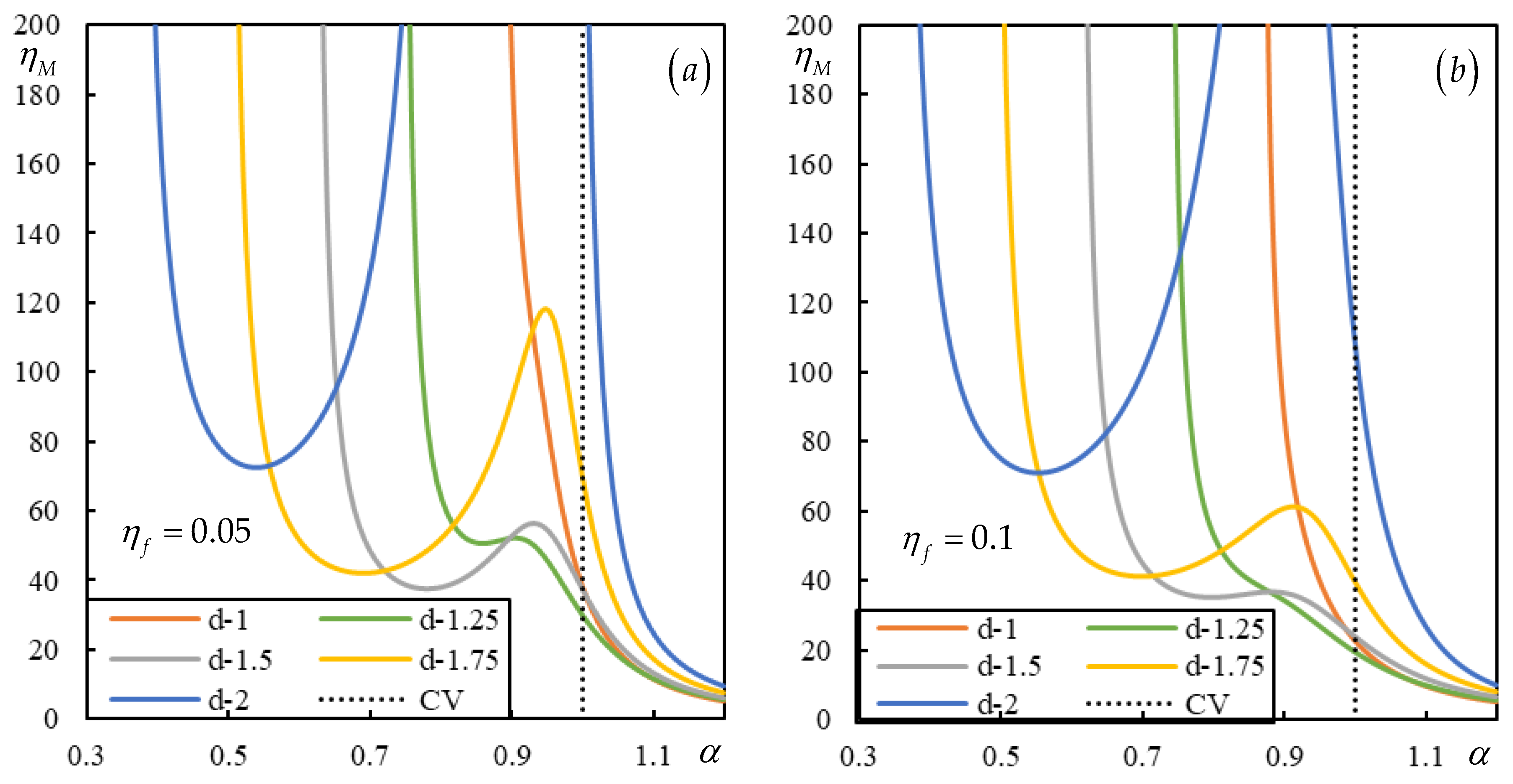
It can be concluded that with increasing damping, all branches of instability shift to lower moving masses and at the same time become straighter, so that lower masses occupy larger velocity intervals. It has thus been proven that contrary to what is generally expected, foundation damping worsens the situation. However, it is necessary to note that in closed intervals the degree of instability is usually much lower than in semi-closed intervals.
In Figure 3 only relevant distances between mases are included, that is those that still have part of the branch within the defined scale in subcritical velocity range. By analyzing a larger range of distances between masses, it can be concluded that the starting point of the first branch of instability shifts to the left with increasing distance, but at the same time the moving masses increase.
When the moving bogie is considered, there are more parameters that can vary. To make the comparison more realistic, the total mass should be the same. The case with is considered in Figure 4 for comparison and thus the previous instability lines from Figure 3 are recalculated accordingly. Besides , the moving bogie is characterized by and to make its influence as less as possible.
It can be concluded that even for weak primary suspension stiffness and low mass moment of inertia of the bogie bar, all cases with moving bogie perform better, meaning the instability lines are above the ones for moving masses, except for the lowest tested distance . Instability lines in Figure 4 are represented only up to the critical velocity. The relevant instability lines are those that have a part of a branch within the chosen scale in the subcritical velocity range. Then the following rule applies: if is relevant for moving masses but not for a moving bogie, then is not plotted for moving masses, even if it is relevant.
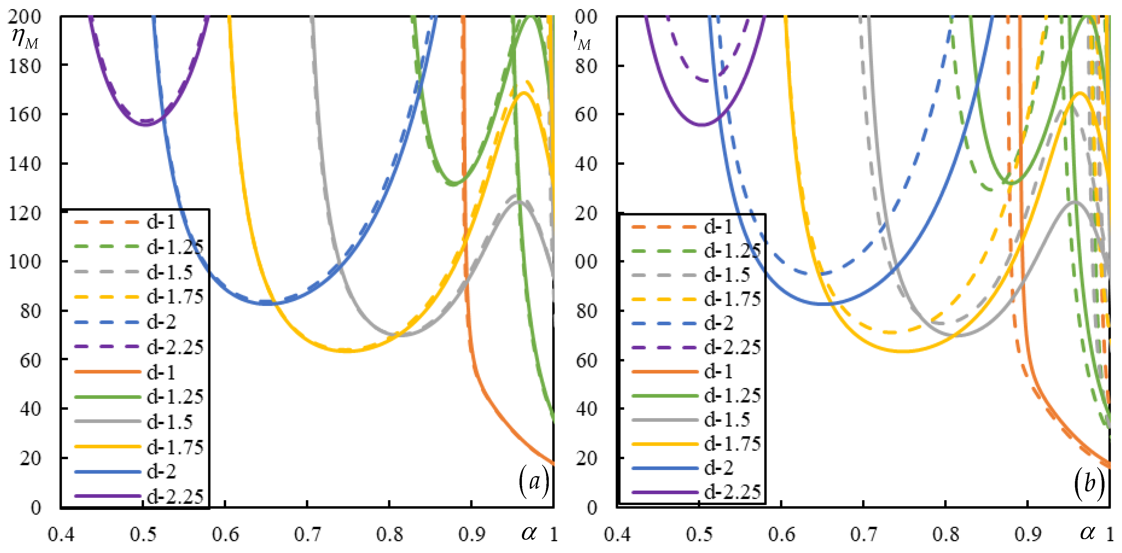
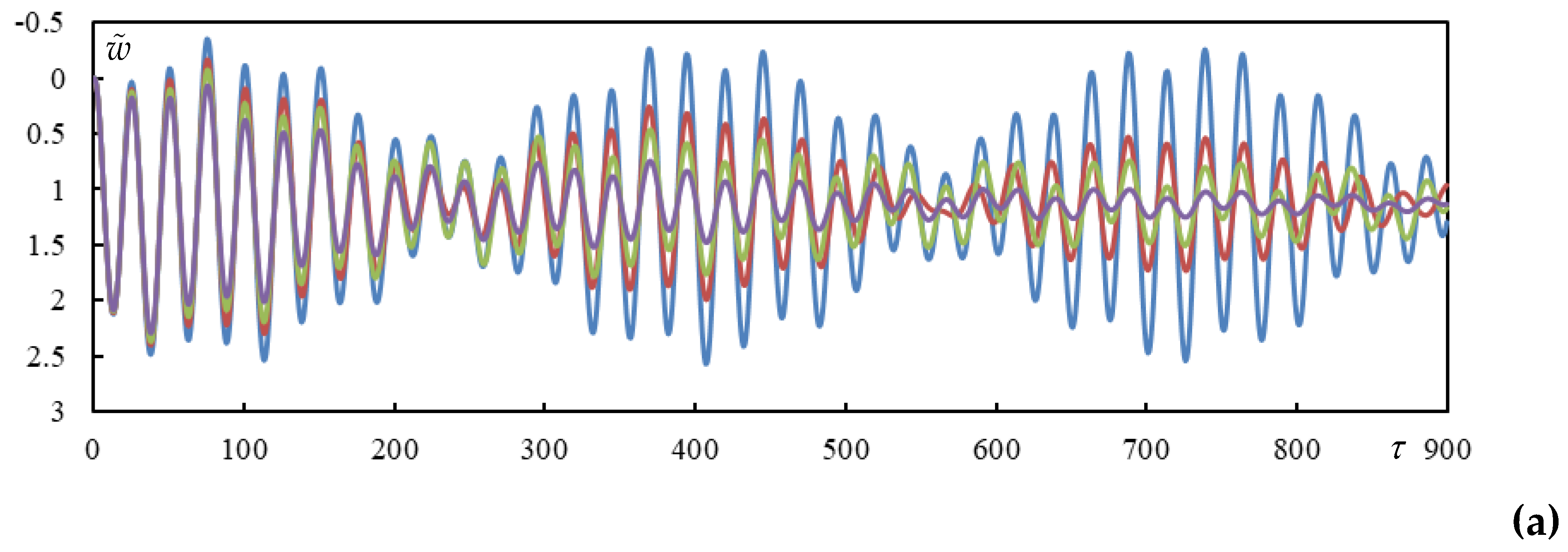
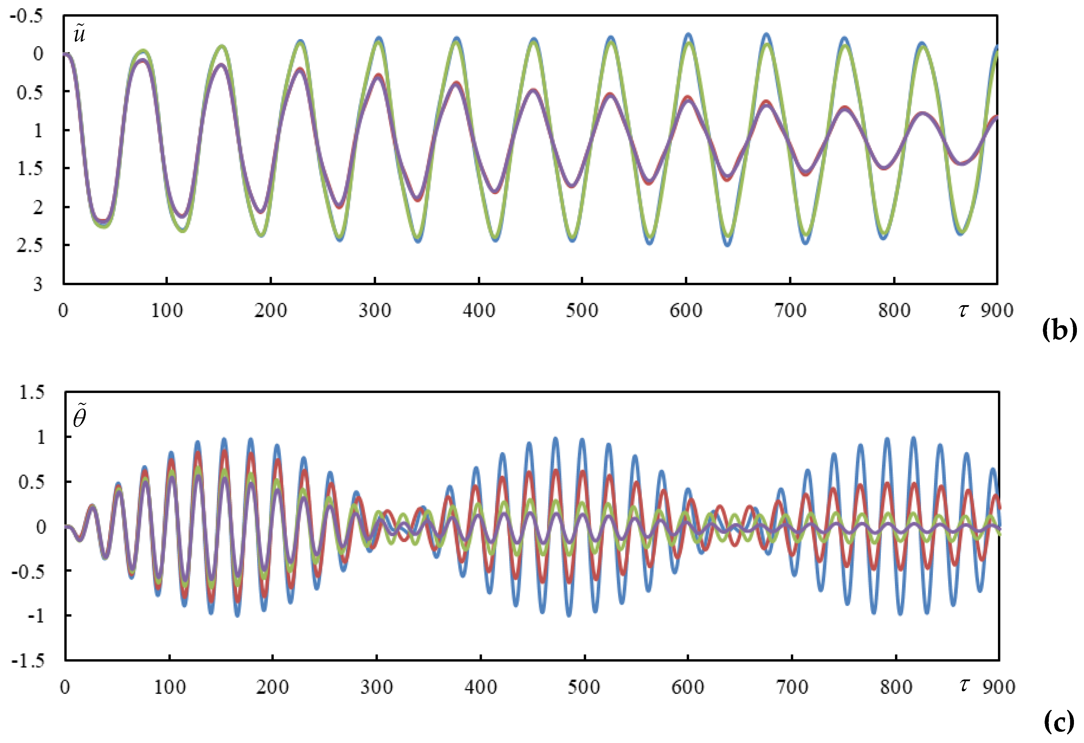
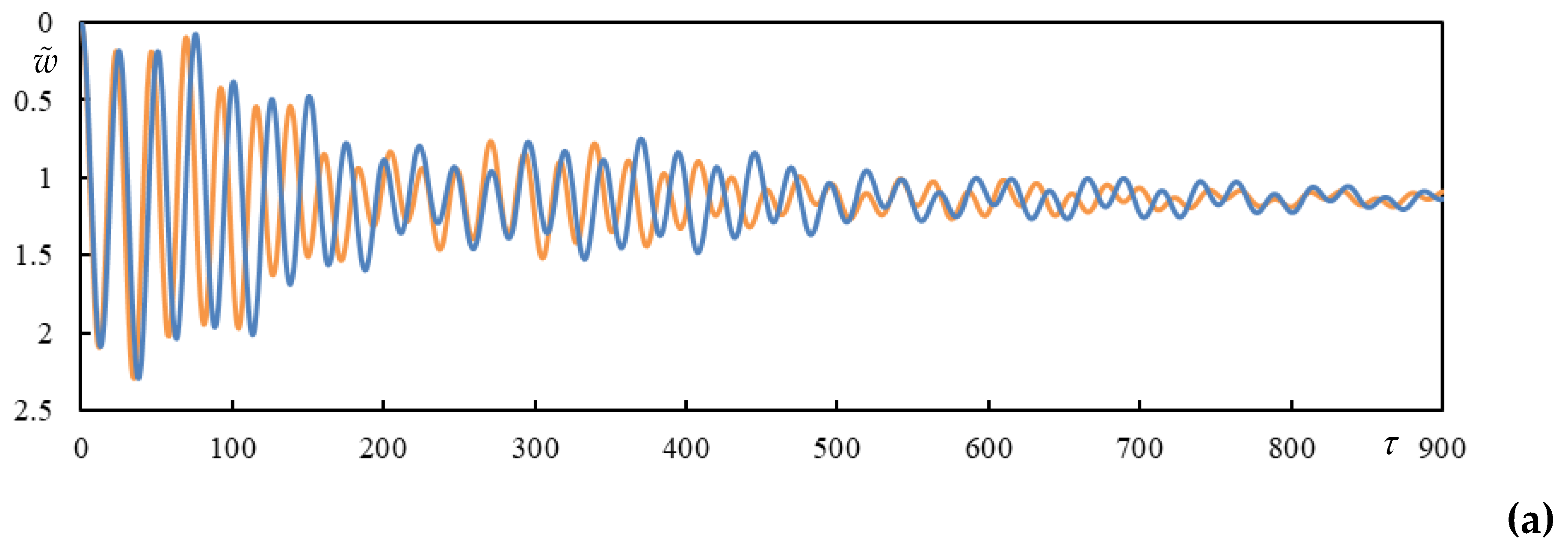
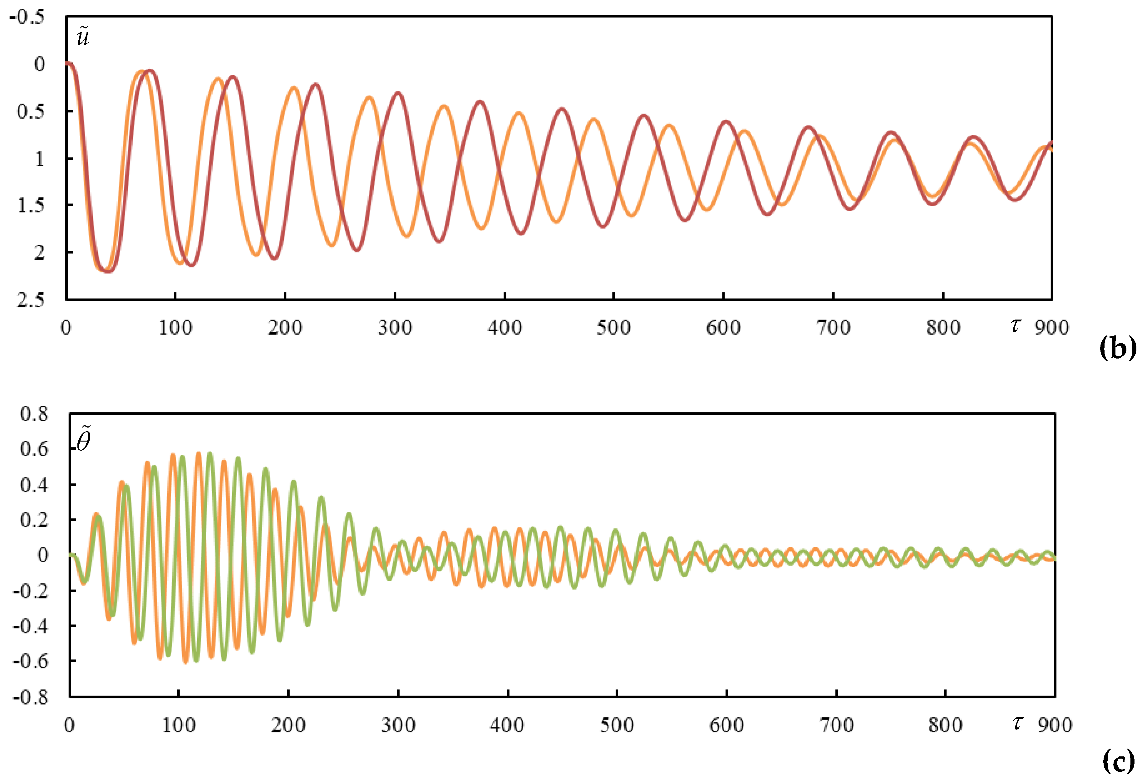
To analyze in detail the only case of moving bogie that performs worse than moving masses, Case 1 from Table 1 is selected. This case is unstable. Nevertheless, as it is seen from Table 2, the unstable frequency has quite a low imaginary part (in absolute value). This means that the unstable frequency is gaining importance only in higher times, while in the beginning this case resembles a highly damped case. In Figure 5 time series are shown, obtained by closed-form formulas and also on finite beam for validation. The high times in Figure 6 are calculated using closed-form formulas only, it would be computationally untenable to do this on a finite beam due to the excessive number of vibration modes and also using numerical integration due to numerical precision.
3.6. Effect of the Suspension Damping
In this section it will be shown that the damping of the suspension has a very positive effect on the bogie stability, moreover this effect is helped by the higher mass moment of inertia of the bogie bar. To demonstrate this, and the other coefficient varies between and . Weak foundation damping of and stiffer primary suspension stiffness of are implemented.
Figure 7 clearly shows that with a higher mass moment of inertia of the bogie bar, practically all instability lines of the cases with primary suspension damping are removed from the subcritical velocity range.
3.6. Effect of the Beam Theory
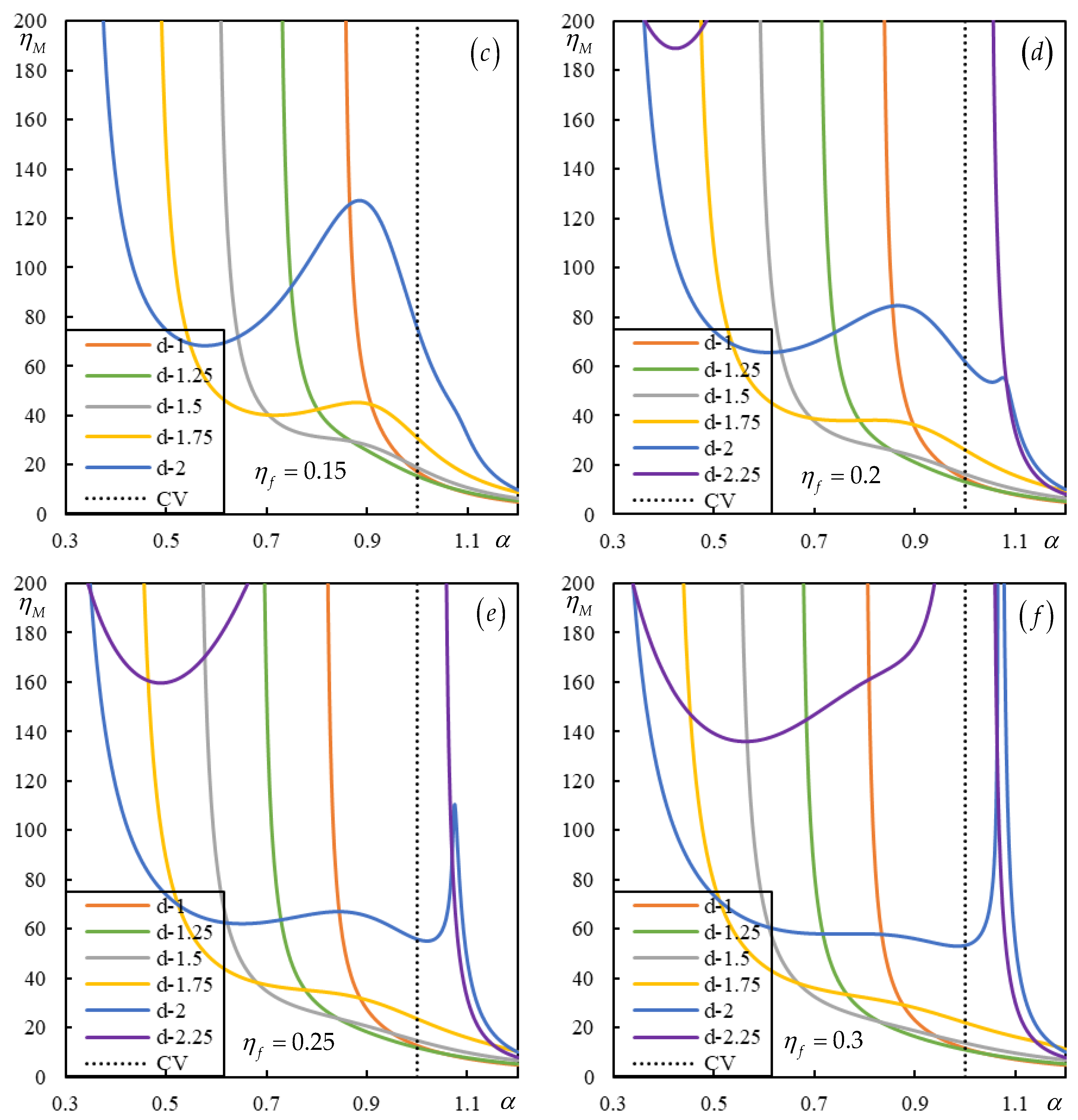
As mentioned earlier, it is also necessary to see how the results are affected by the adopted beam theory. Two cases are shown in Figure 8. The additional parameters of the Timoshenko-Rayleigh beam theory should not be chosen independently, as is clear from Equation (59). Therefore, , are selected for a softer foundation and , for a stronger one. The other parameters are: , . Weak foundation damping of and a stiffer primary suspension stiffness of with no damping are implemented.
Only the subcritical velocity range is shown, However, since the difference in critical velocity in the Timoshenko-Rayleigh case using Equation (66) is very small, 0.993 and 0.980, respectively, the graphs are plotted up to the value 1, as before.
Figure 8.
Instability lines for a moving bogie. Different colors stand for different distances as indicated in the legend. Full curves are for the Euler-Bernoulli theory and dashed curves for the Timoshenko-Rayleigh. (a) , ; (b) , .
Figure 8.
Instability lines for a moving bogie. Different colors stand for different distances as indicated in the legend. Full curves are for the Euler-Bernoulli theory and dashed curves for the Timoshenko-Rayleigh. (a) , ; (b) , .
It can be concluded that for softer foundation there are practically no differences between results obtained using Euler-Bernoulli and Timoshenko-Rayleigh theories. Some differences are noticeable for a stronger foundation, but they do not seem to be fundamental.
3.7. Time Series of Other Cases from Table 1
The objectives of this subsection are threefold, since in addition to the analyzed effect, it is shown how easy it is to use the closed-form formulas, and it is also verified by analysis on finite beams that the contribution of integration along the branch cuts is negligible.
Cases 2 and 3 are selected to show that the dynamic interaction discussed in previous works for two moving masses is maintained for moving bogie. Slightly higher is introduced, but the changes are not significant. Two distances are compared, (Figure 9) and (Figure 10). Other parameters are included in Table 1.
Figure 9 shows a very strong dynamic interaction. In Figure 10 this effect is not as pronounced, however, like for two moving masses, the dynamic interaction persists up to relatively high distances. Only when and start to have negligible values with respect to , then the interaction is negligible. This proves that the function envelopes for still show very strong interaction in Figure 10, because is not included in Equation (43).
Case 4 is selected for comparison with Case 3, to see the effect of with respect to . Besides the time series (Figure 11) it is also interesting to see differences in induced frequencies in Table 2.
Cases 2-4 are undamped; therefore, all amplitudes remain unchanged, the induced frequencies are real (Table 2), and thus these cases also serve to demonstrate how easy it is to deal with undamped cases without numerical problems.
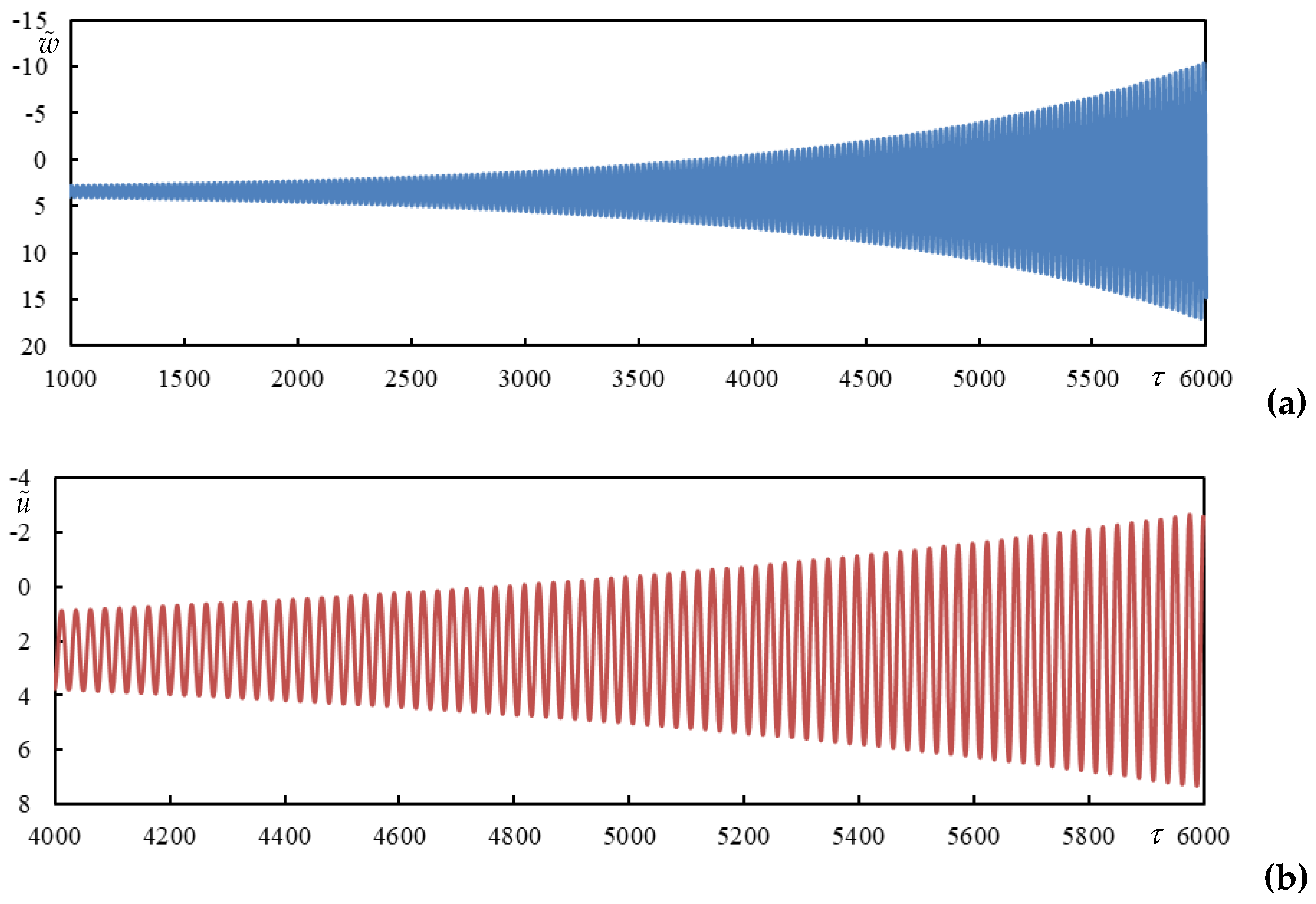
Cases 5 and 6 are chosen such that Case 5 is unstable for subcritical velocity, but by adding damping to the primary suspension and leaving the other parameters unchanged, it becomes stable – Case 6. Time series of Case 5 are reported in Figure 12. During the initial stages there is no indication of instability as the rate of instability is very low (Table 2). The unstable frequency is overpassing the stable ones only at higher times (Figure 13).
Case 6 is already stable. Times series are shown in Figure 14 for initial stages and in Figure 15 for higher times.
The other cases from Table 1 are summarized in Appendix A.
3.8. Comparison with Other Published Works
While in [49] only isolated cases are shown, in [48] an evolution over a range of velocities is presented, which provides a better insight into the problem. Nevertheless, the reference case corresponds to a case with negligible dynamic interaction between the wheels, which is assumed as 15m, so it is not an actual bogie but a simplified vehicle with two axels. The evolution of the critical stiffness of the primary suspension is chosen for comparison. The results are shown in Figure 16 using the input data from [48].
It can be concluded that there is a very good agreement after recalculation to dimensionless data as in [48]. Some minor differences can be justified by the fact that nowadays it is possible to use symbolic software allowing much higher accuracy and faster evaluation than at the time of [48] was written.
4. Discussion
This paper presents a detailed analysis of the instability of a bogie passing through a one-layer model, focusing on the possibility that this may occur in the subcritical velocity range. All presented results were obtained (semi)analytically, quickly and with very high accuracy.
The results of two moving proximate masses are used as a reference case and it is shown that in general, the more realistic the moving object, the lower the risk of instability at such low velocities. This was confirmed even under the conditions of neglected suspension damping, reduced suspension stiffness and small mass moment of inertia of the bogie bar. On the other hand, it was confirmed that the negative effect of foundation damping found in the two moving mass cases is preserved for the moving bogie. This effect is in contrast to the effect of foundation damping in the case of a single moving inertial object, where increased damping always shifts the onset of instability to higher velocities.
It has been demonstrated that instability lines related to moving bogies have more branches than those related to moving masses, which complicates the analysis.
It has been shown that suspension damping improves the unstable behavior in all cases, but it is much more efficient with a higher mass moment of inertia of the bogie bar.
Regarding the distances between the masses: it is not true that the lowest means worse. Larger distances shift the starting point of the first instability branch to lower speeds, but at the same time the smallest moving mass ratio of such branch increases, therefore, it is necessary to balance these two tendencies.
It has been proven that there are cases with realistic parameters where instability occurs in the subcritical velocity range, and therefore this article serves as a warning that instability at supercritical velocities cannot be taken for granted a priori.
Unlike in all other works published by other researchers (e.g. [48,49,50]) where the instability is determined by the D-decomposition method, here the so-called lines of instability are traced in the plane of velocity-moving mass ratios by identifying the real-valued induced frequencies, which in a damped case obligatorily alter by one the number of unstable induced frequencies, so that stable and unstable velocity intervals are clearly visible for any specific moving mass ratio. This approach is much more powerful and simpler than the D-decomposition method.
The presented analysis can be easily extended to other types of supporting structures, since all expressions can be used for more complicated foundation models, simply by replacing Equation (24) with an equation reflecting the new foundation model. There is only one complication, namely that in other foundation models the analytical formulas have limited use, since discontinuities in the K-function do not allow to resolve all the necessary induced frequencies for all velocities. This is only relevant for the time series; the instability lines are not affected. As an alternative for the time series, either numerical integration or finite models can be used.
5. Conclusions
In this paper the possibility of instability in subcritical range of velocities was discussed in detail. The results presented are very easy to use, as the dimensionless parameters cover a wide range of possible scenarios, and the instability lines provide an overall view of the onset or aggravation of unstable behavior or the recovery of stable behavior. Such comprehensive information is very useful, as readers do not have to repeat the calculations and can simply calculate their dimensionless parameters for the case they are analyzing.
The validation of the results on finite volumes is clearly described and easily applicable to other researchers. This is simpler than the numerical integration associated with the inverse Laplace transform.
The unstable induced frequencies compared to the stable ones provide an initial estimate of the degree of instability. Indeed, it can be seen in Table 2 that the unstable frequencies of the selected cases have a relatively low imaginary part (in absolute value). As has been shown, the effect of foundation damping worsens the instability, however, during the initial times it has a very strong impact on the stable frequencies, so that the vibrations initially resemble the heavily damped cases. The unstable frequency only surpasses the stable ones at higher times. This is important for assessing the severity of instability and can be used in vibration mitigation measures. Since the analysis allows the determination of the vibration amplitude, together with the degree of instability, it identifies the time required for the unstable harmonics to overcome the stable ones. For this reason, it is important to have analytical formulas that are not affected by numerical approximations during numerical integration and the time response can be extended as needed.
Author Contributions
not applicable-sole author.
Funding
The author acknowledges Fundação para a Ciência e a Tecnologia (FCT) for its financial support via the project LAETA Base Funding (DOI: 10.54499/UIDB/50022/2020). EEA grant FBR_OC2_45: SMART - Sustainable Maintenance and Rehabilitation of Railway Track is also acknowledged.
Data Availability Statement
All data are contained in the paper.
Acknowledgments
The author acknowledges Fundação para a Ciência e a Tecnologia (FCT) for its financial support via the project LAETA Base Funding (DOI: 10.54499/UIDB/50022/2020). EEA grant FBR_OC2_45: SMART - Sustainable Maintenance and Rehabilitation of Railway Track is also acknowledged.
Conflicts of Interest
The author declares no conflicts of interest. The funders had no role in the design of the study; in the collection, analyses, or interpretation of data; in the writing of the manuscript; or in the decision to publish the results.
Appendix A
The aim of this section is to summarize the time series of additional cases listed in Table 1 that are not discussed in the main text. Cases 7-10 demonstrate the effect of damping at different levels. A low level of 5% is chosen and all four combinations are tested by attributing damping to the foundation and/or primary suspension. Case 7 has damping at both levels, and it is reported in Figure A1.
Figure A1.
Time series in Case 7. Full lines are for finite beam and dashed ones for infinite one calculated using closed-form formulas. (a) beam deflection at the rear mass, (b) bogie bar mass center displacement, (c) bogie bar mass center rotation.
Figure A1.
Time series in Case 7. Full lines are for finite beam and dashed ones for infinite one calculated using closed-form formulas. (a) beam deflection at the rear mass, (b) bogie bar mass center displacement, (c) bogie bar mass center rotation.
Figure A2. compares the four cases together.
Figure 2.
Time series in Cases 7-10. Case 7: violet; Case 8: green; Case 9: red; Case 10: blue. (a) beam deflection at the rear mass, (b) bogie bar mass center displacement, (c) bogie bar mass center rotation.
Figure 2.
Time series in Cases 7-10. Case 7: violet; Case 8: green; Case 9: red; Case 10: blue. (a) beam deflection at the rear mass, (b) bogie bar mass center displacement, (c) bogie bar mass center rotation.
From Figure A2 it can be concluded that, as expected, the foundation damping has a larger influence than the primary suspension damping and that all the curves are approximately in phase. This can also be seen from Table 2, since the real parts of the frequencies are very similar, and the noticeable differences are only in the imaginary parts. The dynamic interaction is also very pronounced.
Case 11 complements Case 7 and shows the difference caused by changing the moving masses representing the wheels from in Case 7 to in Case 11. This is illustrated in Figure A3.
Figure A.3.
Time series in Cases 7 and 11. Case 11: orange. (a) beam deflection at the rear mass, (b) bogie bar mass center displacement, (c) bogie bar mass center rotation.
Figure A.3.
Time series in Cases 7 and 11. Case 11: orange. (a) beam deflection at the rear mass, (b) bogie bar mass center displacement, (c) bogie bar mass center rotation.
It can be seen that now the movements are not in phase because the frequencies are different, lower for higher moving masses and vice versa.
Last two cases, Case 12 and 13, are chosen to demonstrate unstable cases in subcritical velocity range, but contrary to Case 1 or 5, for higher mass moment of inertia of the bogie bar, that is for . In Case 12 the moving mass is rather academic (Figure A4 and Figure A5), while in Case 13 more realistic (Figure A6 and Figure A7). Nevertheless, both cases have again rather low degree of instability, as can be concluded from Table 2 and therefore higher times must be shown to prove the instability (Figure A5 and Figure A7).
Figure A4.
Time series in Case 12. (a) beam deflection at the rear mass, (b) bogie bar mass center displacement, (c) bogie bar mass center rotation.
Figure A4.
Time series in Case 12. (a) beam deflection at the rear mass, (b) bogie bar mass center displacement, (c) bogie bar mass center rotation.
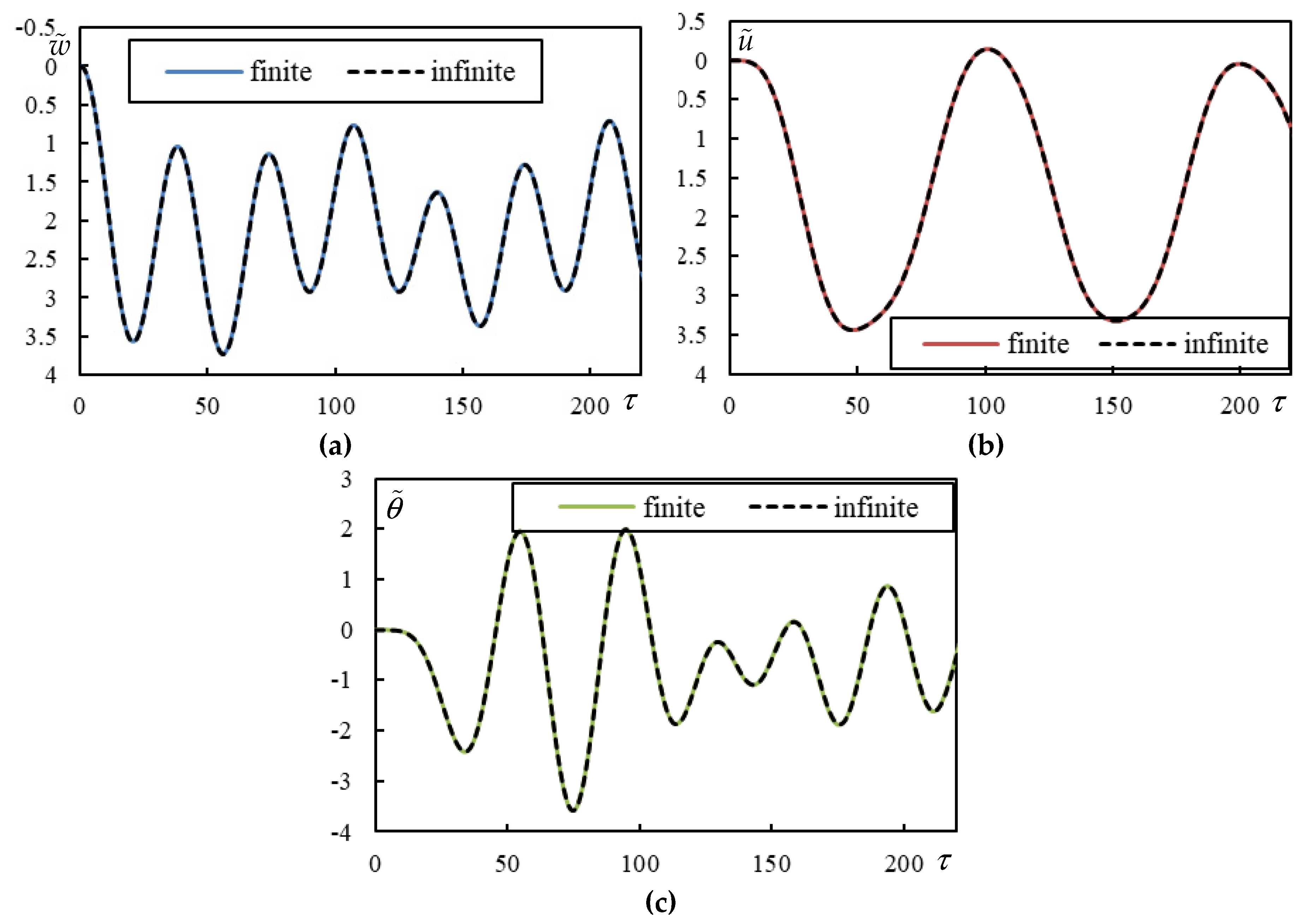
Figure A5.
Time series in Case 12. (a) beam deflection at the rear mass, (b) bogie bar mass center displacement.
Figure A5.
Time series in Case 12. (a) beam deflection at the rear mass, (b) bogie bar mass center displacement.
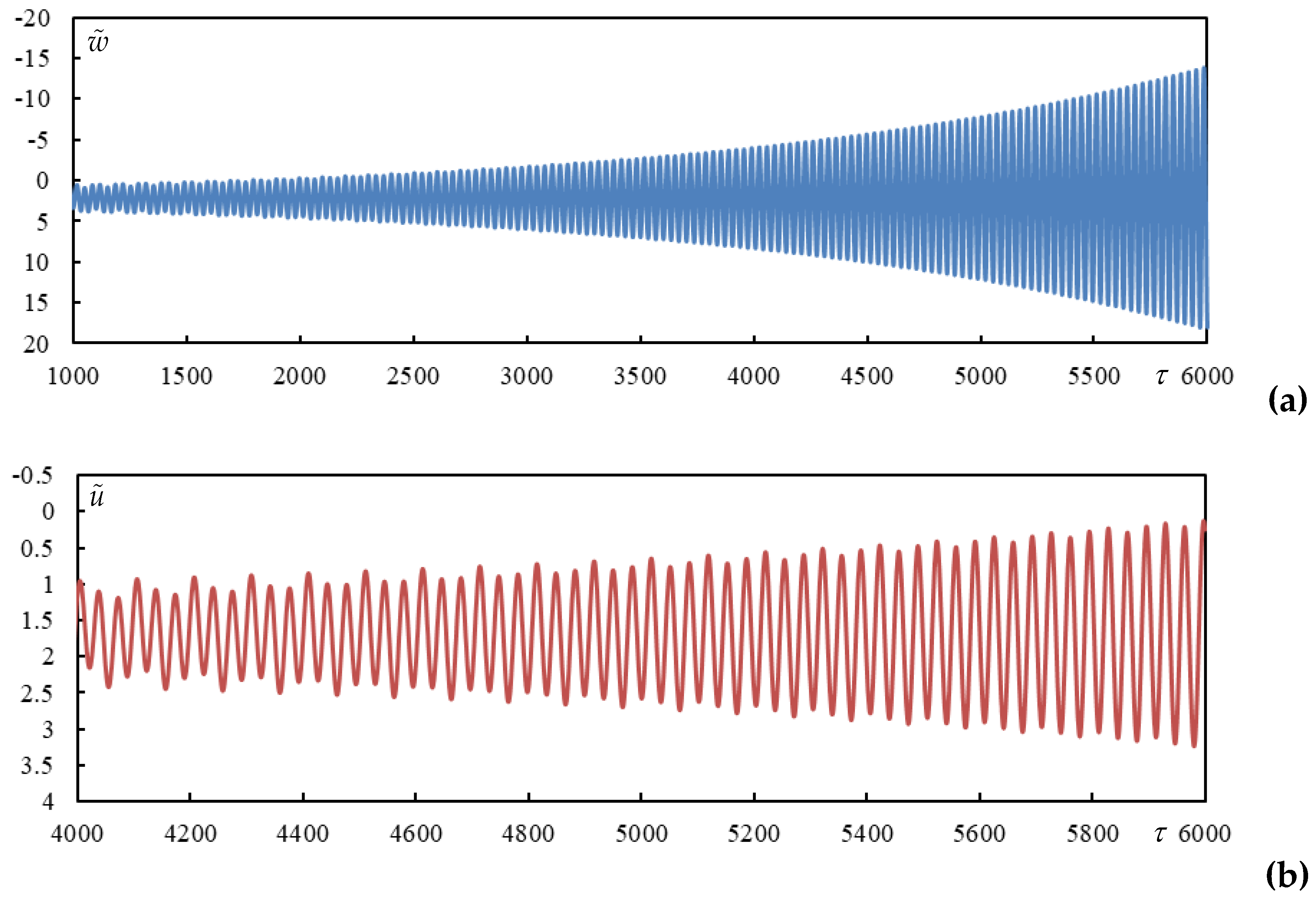
Figure A6.
Time series in Case 13. (a) beam deflection at the rear mass, (b) bogie bar mass center displacement, (c) bogie bar mass center rotation.
Figure A6.
Time series in Case 13. (a) beam deflection at the rear mass, (b) bogie bar mass center displacement, (c) bogie bar mass center rotation.
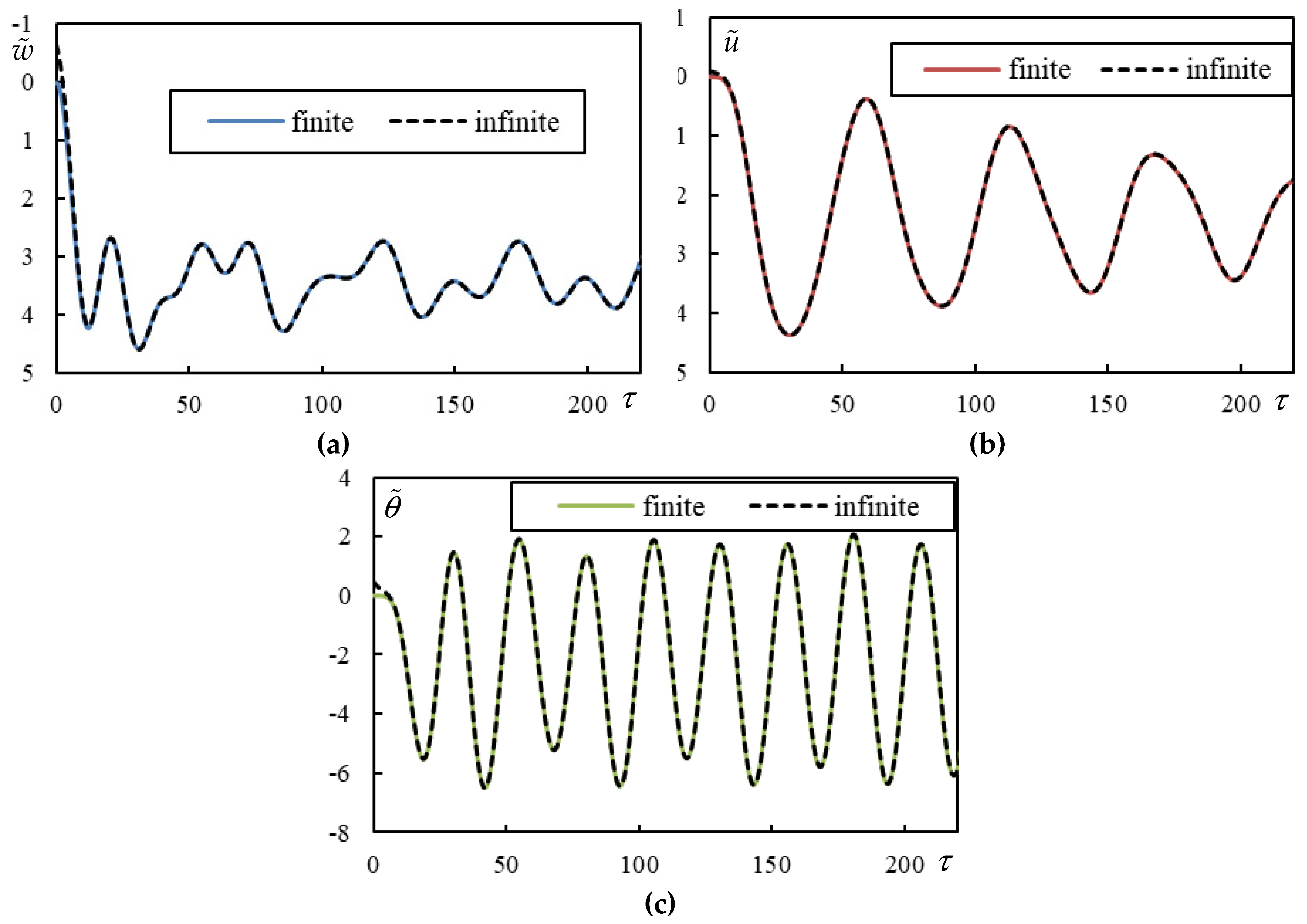
Figure A7.
Time series in Case 13. (a) beam deflection at the rear mass, (b) bogie bar mass center displacement.
Figure A7.
Time series in Case 13. (a) beam deflection at the rear mass, (b) bogie bar mass center displacement.
References
- Rodrigues, A.S.F.; Dimitrovová, Z. Applicability of a three-layer model for the dynamic analysis of ballasted railway tracks. Vibration, 2021, 4, 151-174. [CrossRef]
- Dimitrovová, Z. On the critical velocity of moving force and instability of moving mass in layered railway track models by semianalytical approaches. Vibration 2023, 6, 113-146. [CrossRef]
- Beskou, N.D.; Muho, E.V. Review on dynamic response of road pavements to moving vehicle loads; part 1: Rigid pavements. Soil. Dyn. Earthq. Eng. 2023, 175, 108249. [CrossRef]
- Muho, E.V.; Beskou, N.D. Review on dynamic analysis of road pavements under moving vehicles and plane strain conditions. Journal of Road Engineering 2024, 4(1), 54-68. [CrossRef]
- Dimitrovová, Z. Semi-analytical analysis of vibrations induced by a mass traversing a beam supported by a finite depth foundation with simplified shear resistance. Meccanica 2020, 55, 2353–2389. [CrossRef]
- Ouyang, L.; Xiang, Z.; Zhen, B.; Yuan, W. Analytical Study on the Impact of Nonlinear Foundation Stiffness on Pavement Dynamic Response under Vehicle Action. Appl. Sci. 2024, 14(19), 8705. [CrossRef]
- Hua, X.; Zatar, W.; Cheng, X.; Chen, G.S.; She, Y.; Xu, X.; Liao, Z. Modeling and Characterization of Complex Dynamical Properties of Railway Ballast. Appl. Sci. 2024, 14, 11224. [CrossRef]
- Yang, J.; He, X.; Jing, H.; Wang, H.; Tinmitonde, S. Dynamics of Double-Beam System with Various Symmetric Boundary Conditions Traversed by a Moving Force: Analytical Analyses. Appl. Sci. 2019, 9(6), 1218. [CrossRef]
- Zhao, L.; Wang, S.-L. Analytical determination of critical velocity and frequencies of beam with moving mass under different supporting conditions. J. Vibroeng. 2024, 26(5), 1014-1026. [CrossRef]
- Al-Ashtari, W. A new approach for modelling the vibration of beams under moving load effect. ARPN Journal of Engineering and Applied Sciences 2023, 18(11), 1195–1206.
- Ghannadiasl, A.; Mofid, M. Sensitivity analysis of vibration response of timoshenko beam to mass ratio and velocity of moving mass and boundary conditions: Semi-analytical approach. Forces in Mechanics 2023, 11, 100205. [CrossRef]
- Zhou, R.; Yang, P.; Li, Y.; Tao, Y.G.; Xu, J.; Zhu, Z. Interfacial properties of double-block ballastless track under various environmental conditions. Int. J. Mech. Sci. 2024, 266, 108954. [CrossRef]
- Dumitriu, M. Fault detection of damper in railway vehicle suspension based on the cross-correlation analysis of bogie accelerations. Mech. Ind. 2019, 20, 102. [CrossRef]
- Heydari, H. Evaluating the dynamic behavior of railway-bridge transition zone: numerical and field measurements. Can. J. Civil. Eng. 2024, 51(4), 399-408. [CrossRef]
- Jain, A.; Metrikine, A.V.; Steenbergen, M.J.M.M.; van Dalen, K.N. Railway Transition Zones: Energy Evaluation of a Novel Transition Structure for Critical Loading Conditions. J. Vib. Eng. Technol. 2025, 13(1), 15. [CrossRef]
- Uranjek, M.; Imamović, D.; Peruš, I. Mathematical Modeling of the Floating Sleeper Phenomenon Supported by Field Measurements. Mathematics 2024, 12(19), 3142. [CrossRef]
- Li, Z.; Li, S.; Zhang, P.; Núñez, A.; Dollevoet, R. Mechanism of short pitch rail corrugation: initial excitation and frequency selection for consistent initiation and growth. International Journal of Rail Transportation 2024, 12(1), 13150. [CrossRef]
- Zhang, P.; He, C.; Shen, C.; Dollevoet, R.; Li, Z. Comprehensive validation of three-dimensional finite element modelling of wheel-rail high-frequency interaction via the V-Track test rig. Vehicle Syst. Dyn. 2024, 62(11), 2785-2809. [CrossRef]
- Fărăgău, A.B.; Metrikine, A.V.; van Dalen, K.N. Transition radiation in a piecewise-linear and infinite one-dimensional structure–a Laplace transform method. Nonlinear Dyn. 2019, 98, 2435–2461. [CrossRef]
- Fărăgău, A.B.; Keijdener, C.; de Oliveira Barbosa, J.M.; Metrikine, A.V.; van Dalen, K.N. Transition radiation in a nonlinear and infinite one-dimensional structure: A comparison of solution methods. Nonlinear Dyn. 2021, 103, 1365–1391. [CrossRef]
- Gao, L.; Shi, S.; Zhong, Y.; Xu, M.; Xiao, Y. Real-time evaluation of mechanical qualities of ballast bed in railway tamping maintenance. Int. J. Mech. Sci. 2023, 248, 108192. [CrossRef]
- Yang, Y.B.; Gao, S.Y.; Shi, K.; Mo, X.Q.; Yuan, P.; Wang, H.Y. Selection of the Span Length of an Analogic Finite Beam to Simulate the Infinite Beam Resting on Viscoelastic Foundation Under a Harmonic Moving Load. Int. J. Struct. Stab. Dy. 2024, 2540001. [CrossRef]
- Dimitrovová, Z. Semi-analytical solution for a problem of a uniformly moving oscillator on an infinite beam on a two-parameter visco-elastic foundation. J. Sound Vib. 2019, 438, 257-290. [CrossRef]
- Dimitrovová, Z. A General Procedure for the Dynamic Analysis of Finite and Infinite Beams on Piece-Wise Homogeneous Foundation under Moving Loads. J. Sound Vib. 2010, 329(13), 2635–2653. [CrossRef]
- Dimitrovová, Z. Two-layer model of the railway track: analysis of the critical velocity and instability of two moving proximate masses. Int. J. Mech. Sci. 2022, 217, 107042. [CrossRef]
- Dimitrovová, Z. Complete semi-analytical solution for a uniformly moving mass on a beam on a two-parameter visco-elastic foundation with non-homogeneous initial conditions. Int. J. Mech. Sci. 2018, 144, 283-311. [CrossRef]
- Zhang, S.; Fan, W.; Yang, C. Semi-analytical solution to the steady-state periodic dynamic response of an infinite beam carrying a moving vehicle. Int. J. Mech. Sci. 2022, 226, 107409. [CrossRef]
- Mazilu, T.; Răcănel, I.R.; Gheți, M.A. Vertical interaction between a driving wheelset and track in the presence of the rolling surfaces harmonic irregularities. Romanian Journal of Transport Infrastructure. 2020, 9(2), 38-52. [CrossRef]
- Kiani, K.; Nikkhoo, A. On the limitations of linear beams for the problems of moving mass-beam interaction using a meshfree method. Acta Mech. Sin. 2011, 28, 164–179. [CrossRef]
- Kiani, K.; Nikkhoo, A.; Mehri, B. Prediction capabilities of classical and shear deformable beam models excited by a moving mass. J. Sound Vib. 2009, 320, 632–648. [CrossRef]
- Kiani, K.; Nikkhoo, A.; Mehri, B. Assessing dynamic response of multispan viscoelastic thin beams under a moving mass via generalized moving least square method. Acta Mech. Sin. 2010, 26, 721–733. [CrossRef]
- Jahangiri, A.; Attari, N.K.A.; Nikkhoo, A.; Waezi, Z. Nonlinear dynamic response of an Euler–Bernoulli beam under a moving mass–spring with large oscillations. Arch. Appl. Mech. 2020, 90, 1135–1156. [CrossRef]
- Tran, M.T.; Ang, K.K.; Luong, V.H. Vertical dynamic response of non-uniform motion of high-speed rails. J. Sound Vib. 2014, 333, 5427–5442. [CrossRef]
- Dai, J.; Lim, J.G.Y.; Ang, K.K. Dynamic response analysis of high-speed maglev-guideway system. J. Vib. Eng. Technol. 2023, 11, 2647–2658. [CrossRef]
- Stojanović, V.; Kozić, P.; Petković, M.D. Dynamic instability and critical velocity of a mass moving uniformly along a stabilized infinity beam. Int. J. Solids Struct. 2017, 108, 164–174. [CrossRef]
- Dimitrovová, Z. New semi-analytical solution for a uniformly moving mass on a beam on a two-parameter visco-elastic foundation. Int. J. Mech. Sci. 2017, 127, 142-162. [CrossRef]
- Metrikine, A.V.; Verichev, S.N.; Blaauwendraad, J. Stability of a two-mass oscillator moving on a beam supported by a visco-elastic half-space. Int. J. Solids Struct. 2005, 42, 1187–1207.
- Mazilu, T.; Dumitriu, M.; Tudorache, C. Instability of an oscillator moving along a Timoshenko beam on viscoelastic foundation. Nonlinear Dyn. 2012, 67, 1273–1293. [CrossRef]
- Dimitrovová, Z. Dynamic interaction and instability of two moving proximate masses on a beam on a Pasternak viscoelastic foundation. Appl. Math. Modell. 2021, 100, 192-217. [CrossRef]
- Mazilu, T. Instability of a train of oscillators moving along a beam on a viscoelastic foundation. J. Sound Vib. 2013, 332, 4597–4619. [CrossRef]
- Yang, B.; Gao, H.; Liu, S. Vibrations of a Multi-Span Beam Structure Carrying Many Moving Oscillators. Int. J. Struct. Stab. Dyn. 2018, 18, 1850125. [CrossRef]
- Stojanović, V.; Petković, M.D.; Deng, J. Stability and vibrations of an overcritical speed moving multiple discrete oscillators along an infinite continuous structure. Eur. J. Mech. A/Solids 2019, 75, 367–380. [CrossRef]
- Nassef, A.S.E.; Nassar, M.M.; EL-Refaee, M.M. Dynamic response of Timoshenko beam resting on nonlinear Pasternak foundation carrying sprung masses. Iran. J. Sci. Technol. Trans. Mech. Eng. 2019, 43, 419–426. [CrossRef]
- Stojanović, V.; Petković, M.; Deng, J. Instability of vehicle systems moving along an infinite beam on a viscoelastic foundation. Eur. J. Mech. A. Solids. 2018, 69, 238-254. [CrossRef]
- Dimitrovová, Z. Instability of vibrations of mass(es) moving uniformly on a two-layer track model: Parameters leading to irregular cases and associated implications for railway design. Appl. Sci. 2023, 13, 12356. [CrossRef]
- Yang, C.J.; Xu, Y.; Zhu, W.D.; Fan, W.; Zhang, W.H.; Mei, G.M. A three-dimensional modal theory-based Timoshenko finite length beam model for train-track dynamic analysis. J. Sound Vib. 2020, 479, 115363. [CrossRef]
- Abea, K.; Chidaa, Y.; Quinay, P.E.B., Koroa, K. Dynamic instability of a wheel moving on a discretely supported infinite rail. J. Sound Vib. 2014, 333, 3413–3427. [CrossRef]
- Verichev, S.N.; Metrikine, A.V. Instability of a bogie moving on a flexibly supported Timoshenko beam. J. Sound Vib. 2002, 253(3), 653}668. [CrossRef]
- Stojanović, V.; Deng, J.; Petković, M.; Milić, D. Non-stability of a bogie moving along a specific infinite complex flexibly beam-layer structure. Eng. Struct. 2023, 295, 116788. [CrossRef]
- Stojanović, V.; Deng, J.; Milić, D.; Petković, M.D. Dynamics of moving coupled objects with stabilizers and unconventional couplings. J. Sound Vib. 2024, 570, 118020. [CrossRef]
- Dimitrovová, Z.; Rodrigues, A.F.S. Critical Velocity of a Uniformly Moving Load. Adv. Eng. Softw. 2012, 50, 44–56. [CrossRef]
Figure 1.
One-layer model: (a) traversed by two masses; (b) traversed by a single bogie.
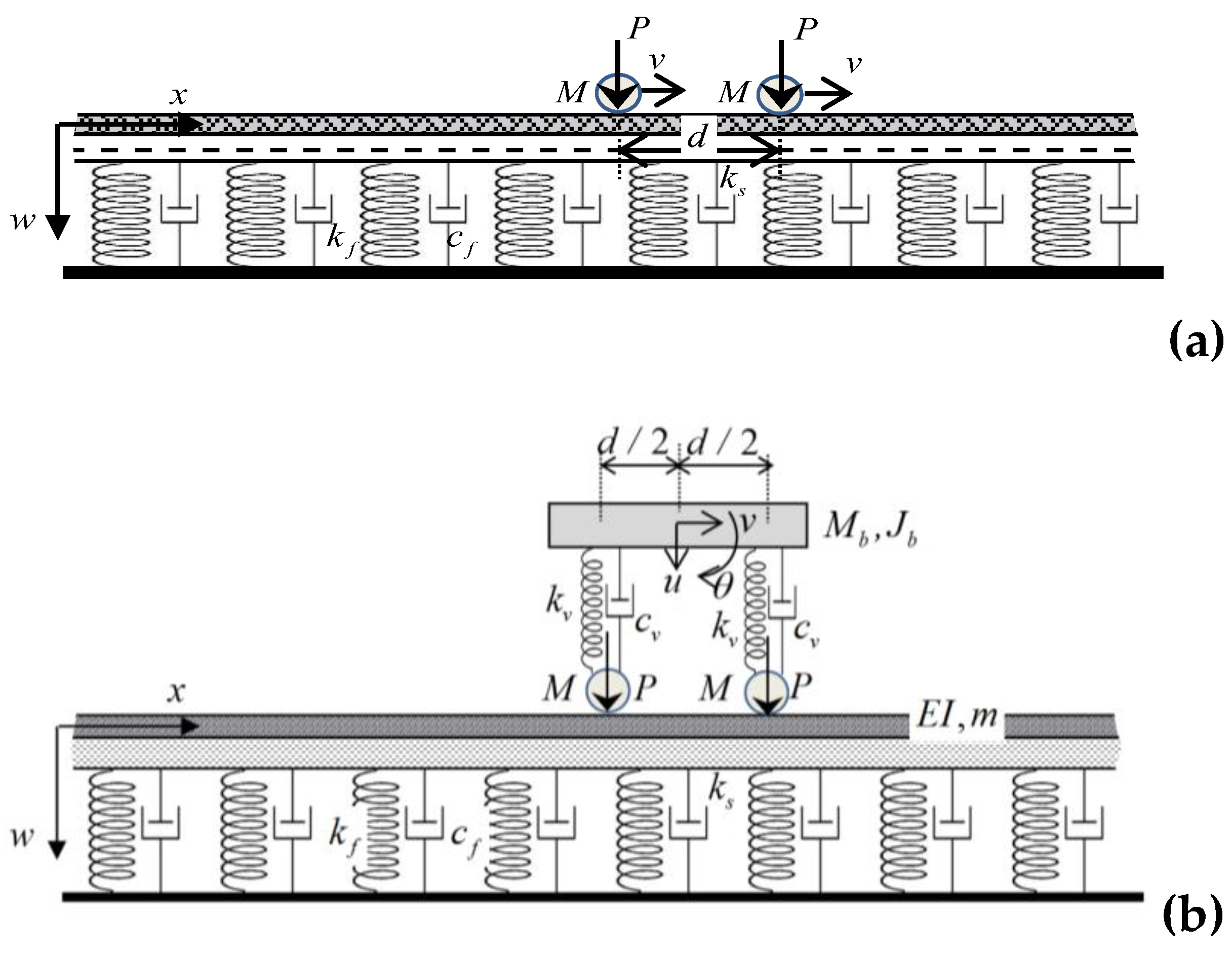
Figure 2.
The real (blue) and imaginary (orange) parts of the induced frequencies in Case 1. Only one root of each pair is plotted, the other root has equal imaginary part but opposite real part.
Figure 2.
The real (blue) and imaginary (orange) parts of the induced frequencies in Case 1. Only one root of each pair is plotted, the other root has equal imaginary part but opposite real part.
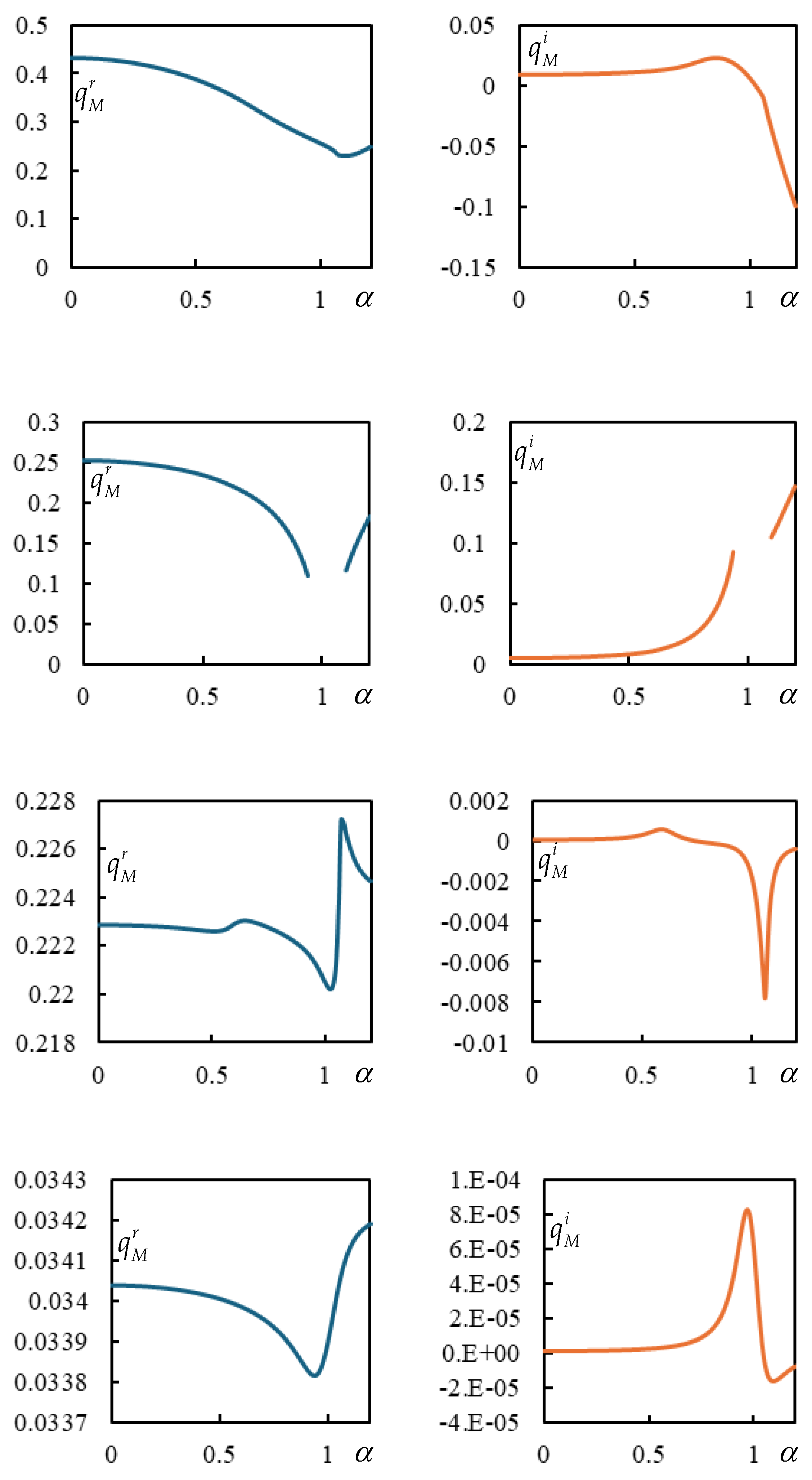
Figure 4.
Instability lines. Different colors stand for different distances as indicated in the legend. Full lines are for a moving bogie and dashed lines for two moving masses, ‘a’ means that these curves were adapted to represent the same total mass. Parts (a) to (f) correspond to .
Figure 4.
Instability lines. Different colors stand for different distances as indicated in the legend. Full lines are for a moving bogie and dashed lines for two moving masses, ‘a’ means that these curves were adapted to represent the same total mass. Parts (a) to (f) correspond to .
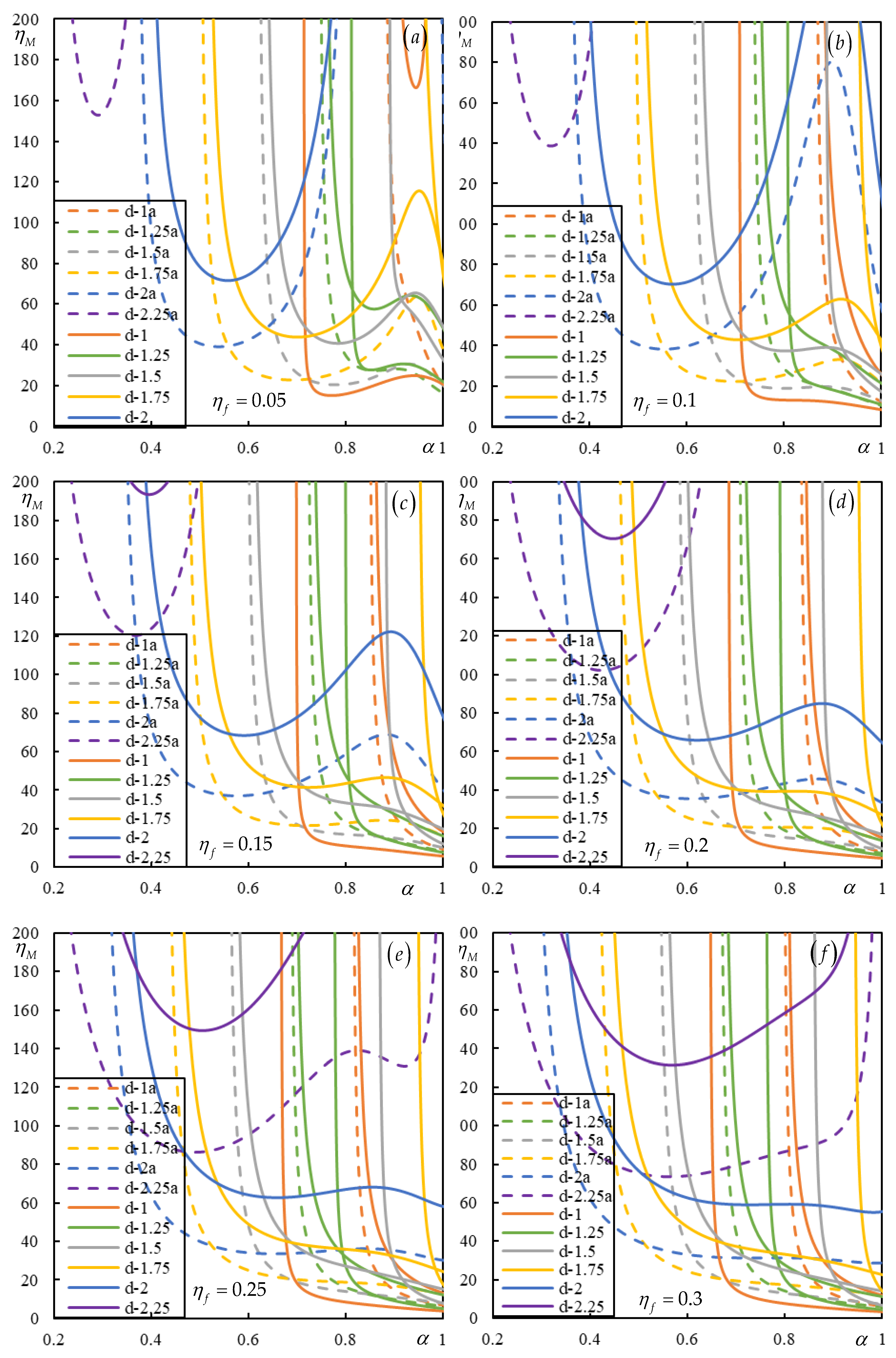
Figure 5.
Time series in Case1. Full lines are for finite beam and dashed ones for infinite one calculated using closed-form formulas. (a) beam deflection at the rear mass, (b) bogie bar mass center displacement, (c) bogie bar mass center rotation.
Figure 5.
Time series in Case1. Full lines are for finite beam and dashed ones for infinite one calculated using closed-form formulas. (a) beam deflection at the rear mass, (b) bogie bar mass center displacement, (c) bogie bar mass center rotation.
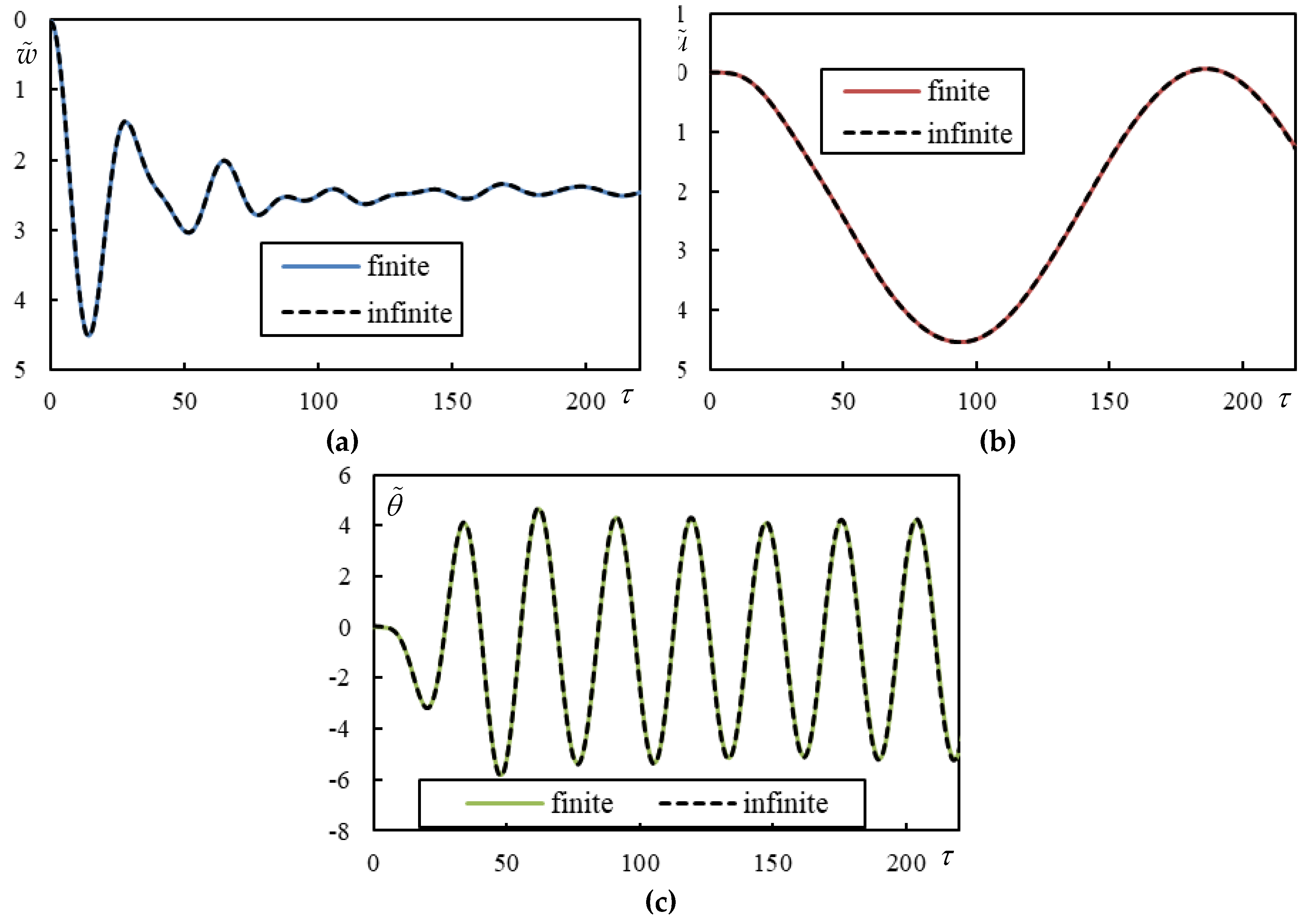
Figure 6.
Time series in Case1. (a) beam deflection at the rear mass, (b) bogie bar mass center displacement.
Figure 6.
Time series in Case1. (a) beam deflection at the rear mass, (b) bogie bar mass center displacement.
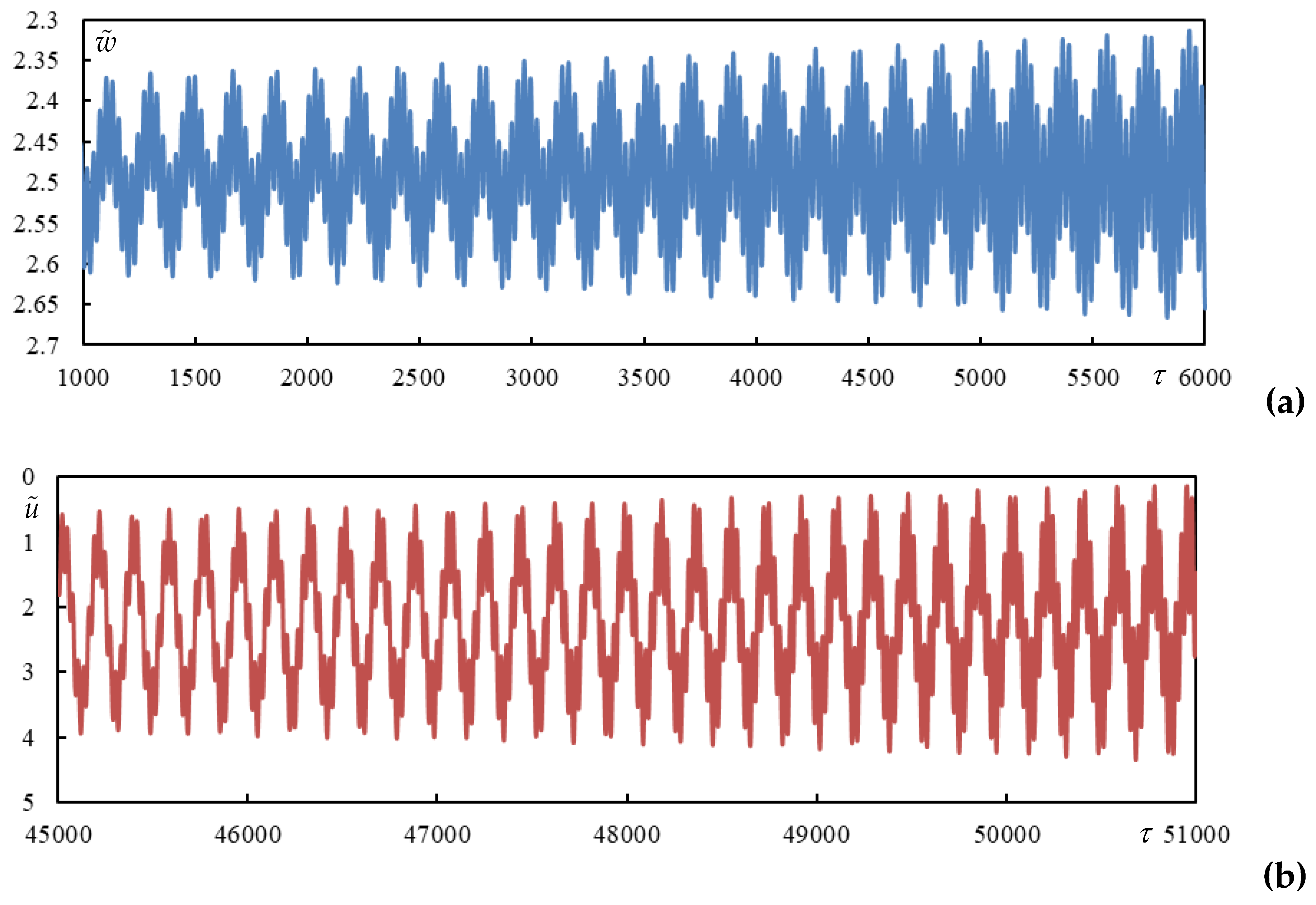
Figure 7.
Instability lines for a moving bogie. Different colors stand for different distances as indicated in the legend. Full curves are for no damping in suspension and dashed curves are for suspension damping of . (a) ; (b) .
Figure 7.
Instability lines for a moving bogie. Different colors stand for different distances as indicated in the legend. Full curves are for no damping in suspension and dashed curves are for suspension damping of . (a) ; (b) .
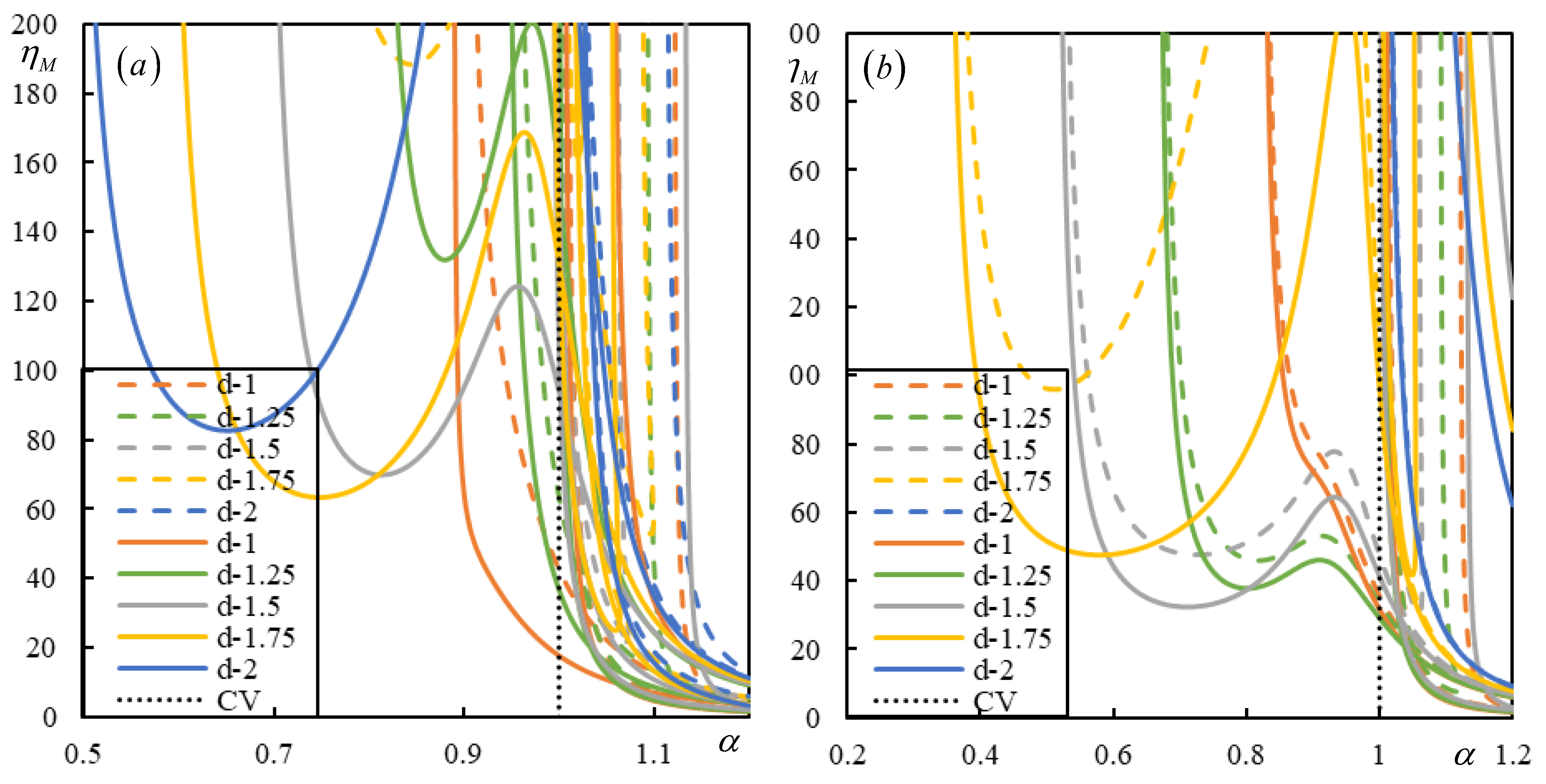
Figure 9.
Time series in Case 2. Full lines are for finite beam and dashed ones for infinite one calculated using closed-form formulas. (a) beam deflection at the rear mass, (b) bogie bar mass center displacement, (c) bogie bar mass center rotation.
Figure 9.
Time series in Case 2. Full lines are for finite beam and dashed ones for infinite one calculated using closed-form formulas. (a) beam deflection at the rear mass, (b) bogie bar mass center displacement, (c) bogie bar mass center rotation.
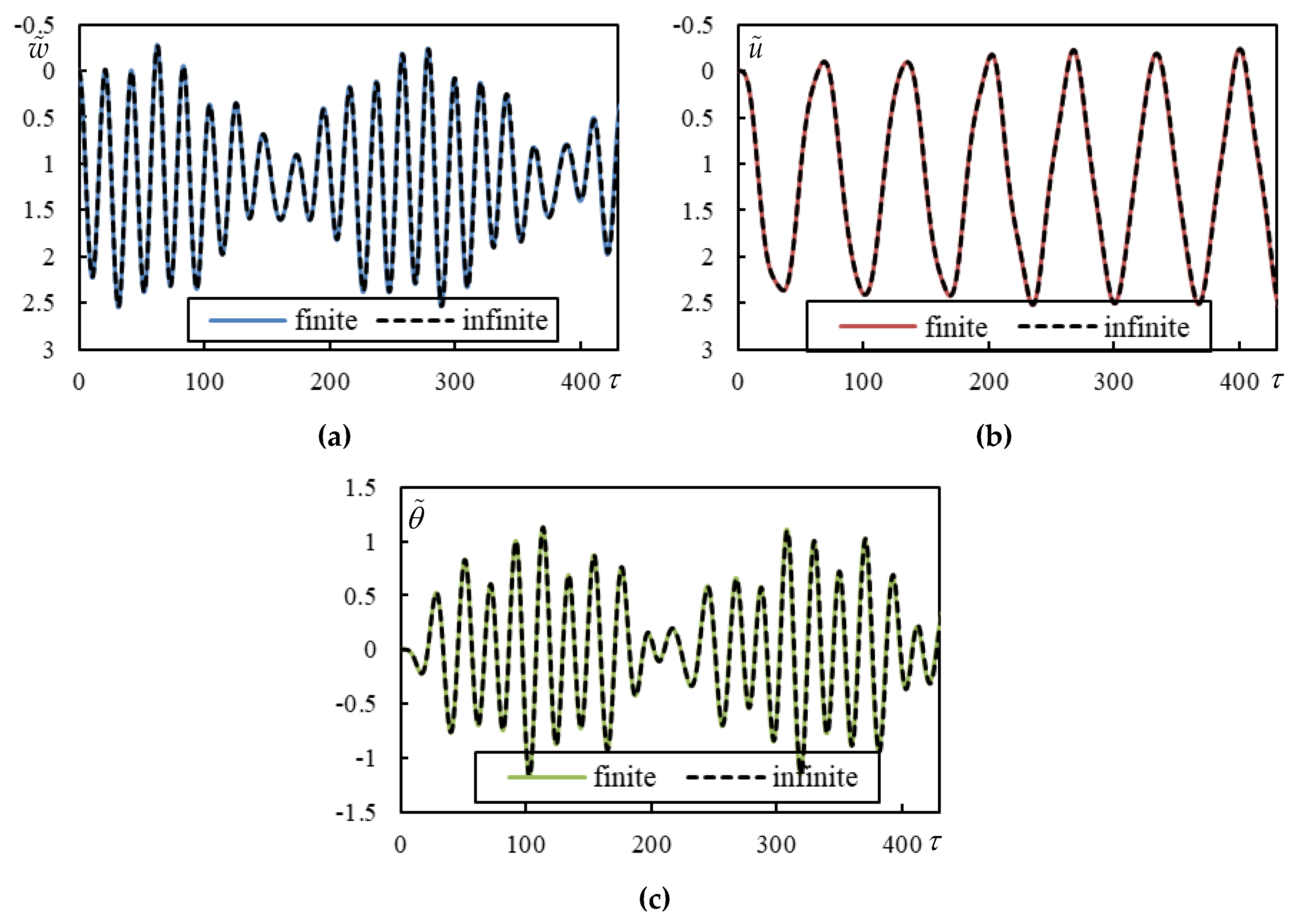
Figure 10.
Time series in Case 3. Full lines are for finite beam and dashed ones for infinite one calculated using closed-form formulas. (a) beam deflection at the rear mass, (b) bogie bar mass center displacement, (c) bogie bar mass center rotation.
Figure 10.
Time series in Case 3. Full lines are for finite beam and dashed ones for infinite one calculated using closed-form formulas. (a) beam deflection at the rear mass, (b) bogie bar mass center displacement, (c) bogie bar mass center rotation.
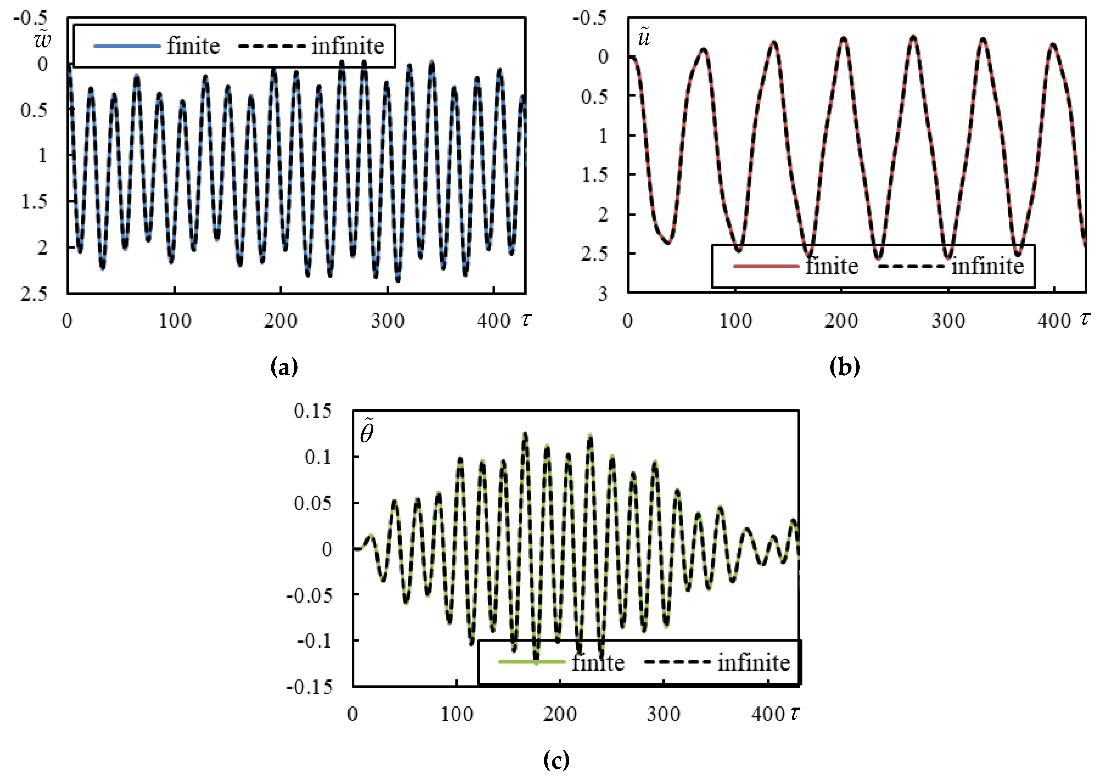
Figure 11.
Time series in Case 4. Full lines are for finite beam and dashed ones for infinite one calculated using closed-form formulas. (a) beam deflection at the rear mass, (b) bogie bar mass center displacement, (c) bogie bar mass center rotation.
Figure 11.
Time series in Case 4. Full lines are for finite beam and dashed ones for infinite one calculated using closed-form formulas. (a) beam deflection at the rear mass, (b) bogie bar mass center displacement, (c) bogie bar mass center rotation.
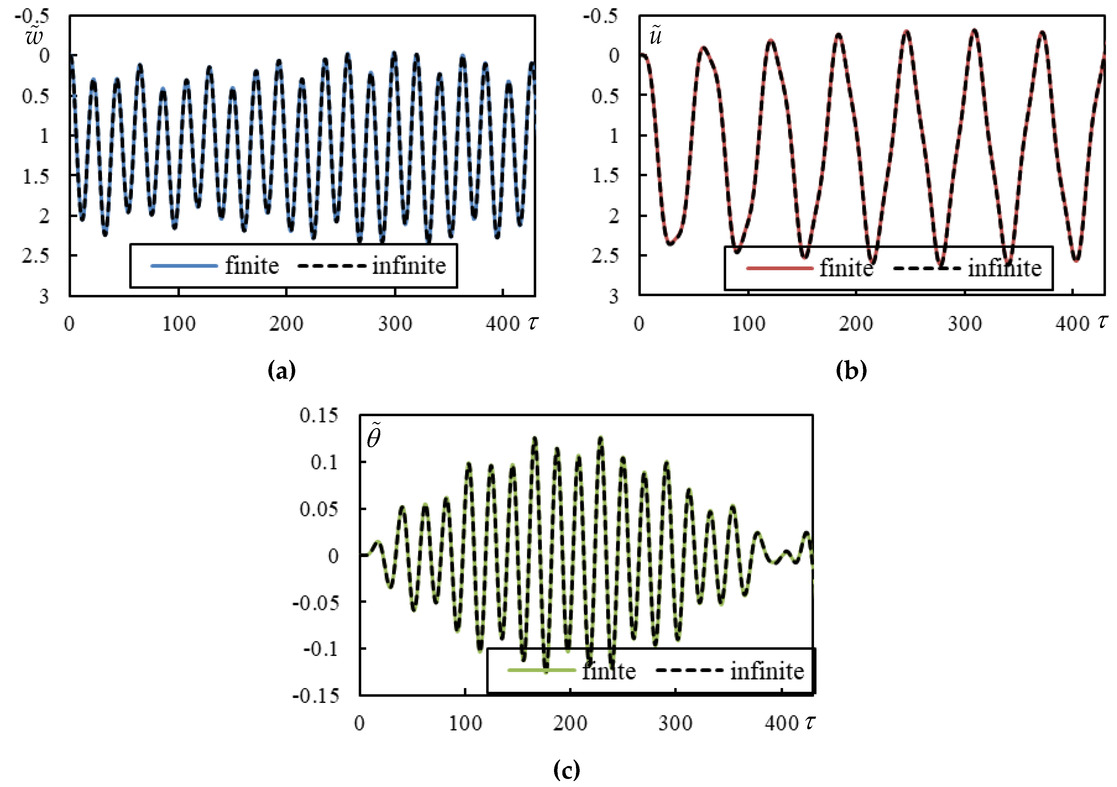
Figure 12.
Time series in Case 5. Full lines are for finite beam and dashed ones for infinite one calculated using closed-form formulas. (a) beam deflection at the rear mass, (b) bogie bar mass center displacement, (c) bogie bar mass center rotation.
Figure 12.
Time series in Case 5. Full lines are for finite beam and dashed ones for infinite one calculated using closed-form formulas. (a) beam deflection at the rear mass, (b) bogie bar mass center displacement, (c) bogie bar mass center rotation.
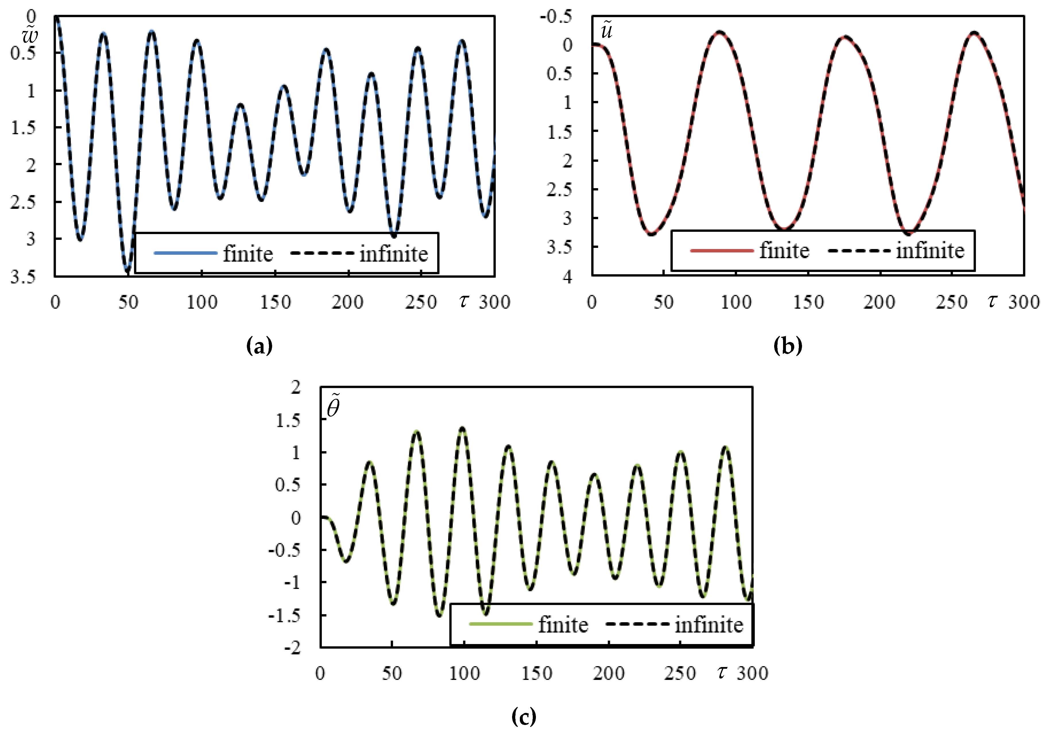
Figure 13.
Beam deflection at the rear mass in Case 5.
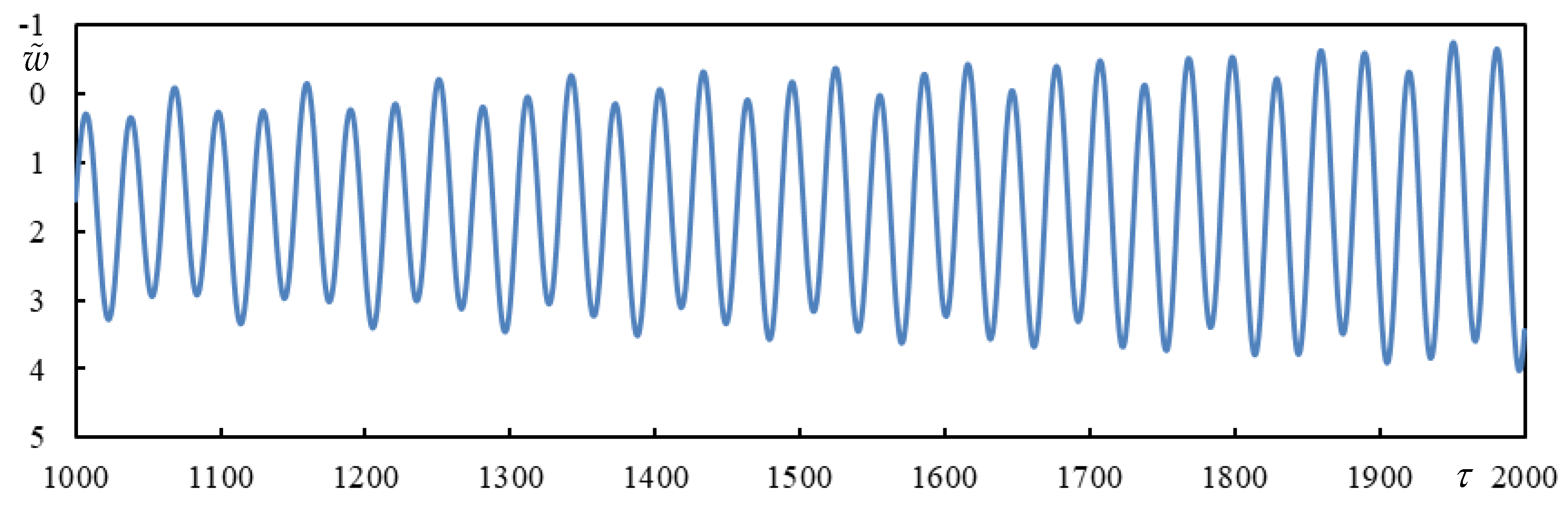
Figure 14.
Time series in Case 6. Full lines are for finite beam and dashed ones for infinite one calculated using closed-form formulas. (a) beam deflection at the rear mass, (b) bogie bar mass center displacement, (c) bogie bar mass center rotation.
Figure 14.
Time series in Case 6. Full lines are for finite beam and dashed ones for infinite one calculated using closed-form formulas. (a) beam deflection at the rear mass, (b) bogie bar mass center displacement, (c) bogie bar mass center rotation.
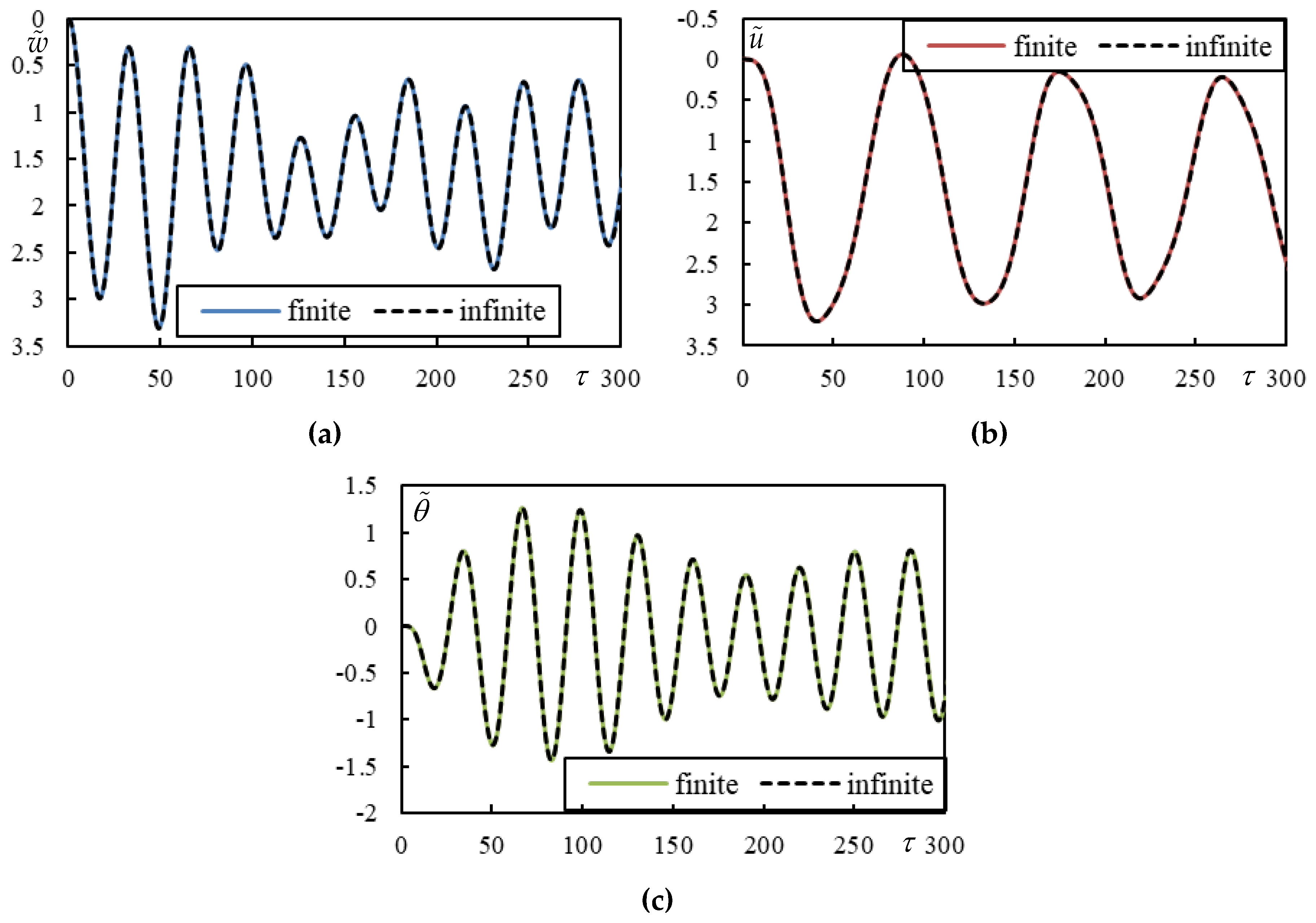
Figure 15.
Beam deflection at the rear mass in Case 6.
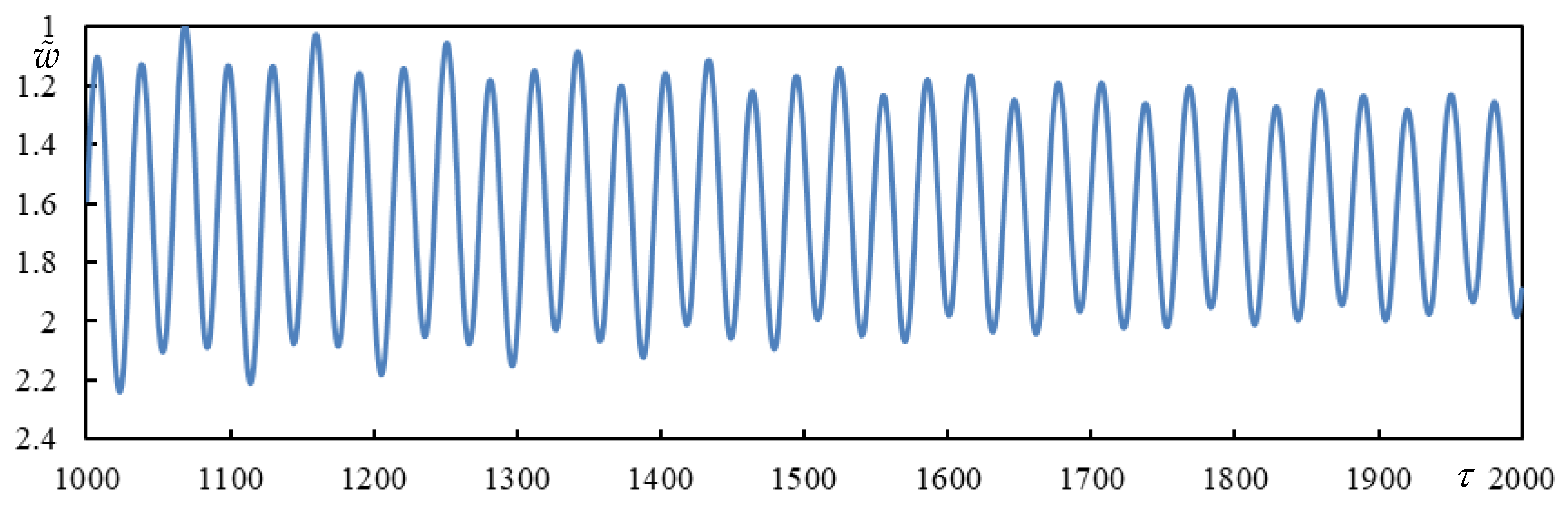
Figure 16.
Critical stiffness of the primary suspension using data from [48].
Figure 16.
Critical stiffness of the primary suspension using data from [48].
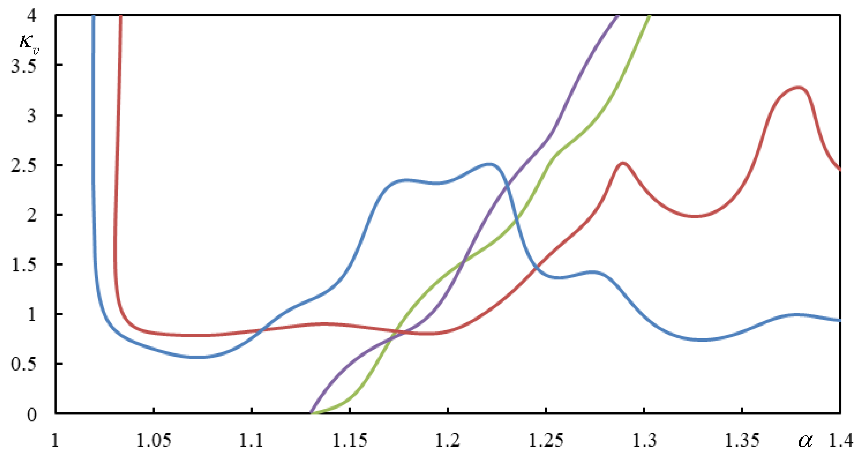

Table 1.
Input data of cases analyzed in time series.
| Parameter | ||||||||
| Case 1 | 0.1 | 20 | 1 | 1.7 | 0.01 | 0.02 | 0 | 0.8 |
| Case 2 | 0 | 20 | 2 | 2 | 0.1 | 0.2 | 0 | 0.5 |
| Case 3 | 0 | 20 | 5 | 2 | 0.1 | 0.2 | 0 | 0.5 |
| Case 4 | 0 | 20 | 5 | 1.7 | 0.1 | 0.2 | 0 | 0.5 |
| Case 5 | 0.05 | 40 | 1.5 | 1.7 | 0.01 | 0.2 | 0 | 0.7 |
| Case 6 | 0.05 | 40 | 1.5 | 1.7 | 0.01 | 0.2 | 0.05 | 0.7 |
| Case 7 | 0.05 | 30 | 2 | 1.7 | 0.01 | 0.2 | 0.05 | 0.4 |
| Case 8 | 0.05 | 30 | 2 | 1.7 | 0.01 | 0.2 | 0 | 0.4 |
| Case 9 | 0 | 30 | 2 | 1.7 | 0.01 | 0.2 | 0.05 | 0.4 |
| Case 10 | 0 | 30 | 2 | 1.7 | 0.01 | 0.2 | 0 | 0.4 |
| Case 11 | 0.05 | 25 | 2 | 1.7 | 0.01 | 0.2 | 0.05 | 0.4 |
| Case 12 | 0.15 | 50 | 1.5 | 1.7 | 0.1 | 0.2 | 0 | 0.85 |
| Case 13 | 0.15 | 15 | 1 | 1.7 | 0.1 | 0.2 | 0 | 0.95 |
Table 2.
Induced frequencies of analyzed cases.
| Parameter | ||||||||
| Case 1 | ±0.307227 | 0.021025 | ±0.222538 | -0.000130 | ±0.184817 | 0.028535 | ±0.033910 | 0.000014 |
| Case 2 | ±0.319059 | 0 | ±0.290698 | 0 | ±0.200435 | 0 | ±0.094072 | 0 |
| Case 3 | ±0.310632 | 0 | ±0.294334 | 0 | ±0.200910 | 0 | ±0.094035 | 0 |
| Case 4 | ±0.310639 | 0 | ±0.294718 | 0 | ±0.200910 | 0 | ±0.101860 | 0 |
| Case 5 | ±0.505305 | 0.000454 | ±0.206528 | -0.000472 | ±0.174711 | 0.007546 | ±0.070460 | 0.000121 |
| Case 6 | ±0.501188 | 0.063327 | ±0.206521 | 0.000448 | ±0.174683 | 0.008301 | ±0.070451 | 0.001137 |
| Case 7 | ±0.577601 | 0.084896 | ±0.255723 | 0.003197 | ±0.236572 | 0.004611 | ±0.083388 | 0.001565 |
| Case 8 | ±0.583823 | 0.000110 | ±0.255859 | 0.001562 | ±0.236478 | 0.004163 | ±0.083397 | 0.000047 |
| Case 9 | ±0.577617 | 0.084792 | ±0.255809 | 0.001646 | ±0.236376 | 0.000436 | ±0.083390 | 0.001518 |
| Case 10 | ±0.583817 | 0 | ±0.255864 | 0 | ±0.236346 | 0 | ±0.083394 | 0 |
| Case 11 | ±0.631225 | 0.101825 | ±0.279230 | 0.003868 | ±0.257027 | 0.005435 | ±0.091336 | 0.001877 |
| Case 12 | ±0.186008 | -0.000482 | ±0.148407 | 0.016963 | ±0.122981 | 0.013168 | ±0.062675 | 0.000636 |
| Case 13 | ±0.354144 | 0.025958 | ±0.249576 | -0.000631 | ±0.167778 | 0.148504 | ±0.113114 | 0.004749 |
Disclaimer/Publisher’s Note: The statements, opinions and data contained in all publications are solely those of the individual author(s) and contributor(s) and not of MDPI and/or the editor(s). MDPI and/or the editor(s) disclaim responsibility for any injury to people or property resulting from any ideas, methods, instructions or products referred to in the content. |
© 2025 by the authors. Licensee MDPI, Basel, Switzerland. This article is an open access article distributed under the terms and conditions of the Creative Commons Attribution (CC BY) license (http://creativecommons.org/licenses/by/4.0/).
Copyright: This open access article is published under a Creative Commons CC BY 4.0 license, which permit the free download, distribution, and reuse, provided that the author and preprint are cited in any reuse.


