Submitted:
18 January 2025
Posted:
21 January 2025
You are already at the latest version
Abstract
SAR target detection and signal detection are critical tasks in electromagnetic signal processing, with wide-ranging applications in remote sensing and communication monitoring. However, these tasks are challenged by complex backgrounds, multi-scale target variations, and the limited integration of domain-specific priors into existing deep learning models. To address these challenges, we propose Refined Deformable-DETR, a novel Transformer-based method designed to enhance detection performance in SAR and signal processing scenarios. Our approach integrates three key components, including the Half-Window Filter (HWF) to leverage SAR and signal priors, the Multi-Scale Adapter to ensure robust multi-level feature representation, and Auxiliary Feature Extractors to enhance feature learning. Together, these innovations significantly enhance detection precision and robustness. The Refined Deformable-DETR achieves a mAP of 0.682 on the HRSID dataset and 0.540 on the Spectrograms dataset, demonstrating remarkable performance compared to other methods.
Keywords:
SAR target detection
; signal detection
; Refined Deformable-DETR
; Half-Window Filter
; Multi-Scale Adapter
; Auxiliary Feature Extractors
1. Introduction
Radar, particularly Synthetic Aperture Radar (SAR), is a tool that detects the distance, velocity, and altitude of objects by emitting electromagnetic waves, offering advantages over traditional optical sensors [1,2]. In recent years, with the advancement of SAR imaging technology and the improvement of image resolution, SAR target detection has become a hot topic, being part of SAR image post-processing. The goal of SAR target detection is to extract the orientation and location of targets from complex scenes quickly and effectively. This is crucial for Synthetic Aperture Radar automatic target recognition, where the accuracy of detection determines the success of subsequent tasks. This study is applicable to not only SAR target detection but also signal detection, aiming to enhance the ability to identify signals and targets in complex electromagnetic environments through deep learning techniques. Signal detection and recognition in dynamic electromagnetic environments is a critical field of study within electronic engineering, driven by the exponential growth of wireless technology usage across sectors. In a wireless monitoring system, signal detection is fundamental and important, serving as the basis for signal recognition, direction, and spectral analysis. However, the electromagnetic environment is complex, presenting significant challenges to detection. Signal detection can be divided into time and frequency domain detection. Additionally, deep learning has demonstrated superior performance in signal detection, enabling automatic feature extraction, improving detection accuracy. Wireless radio signal classification and modulation recognition are crucial issues in intelligent signal processing, holding significance for managing electromagnetic spectrum resources and ensuring reliability and security of communication systems. Researchers have proposed various methods for wireless radio signal identification to improve classification and modulation recognition accuracy.
In recent years, deep learning has been extensively applied across various industries, demonstrating superior performance relative to traditional methods. Many researchers globally have incorporated deep learning techniques into signal detection. O’Shea pioneered using convolutional neural networks (CNN) [3] and deep neural networks (DNN) in radio communications for feature learning and signal recognition [4]. Deep learning-based signal recognition methods typically utilize the spectro-temporal image obtained after short-time Fourier transformation (STFT) [5] as input and output the spectro-temporal information. Prasad et al. [5] used a reduced version of Faster-RCNN [6] for radio signal detection to reduce network size. Another study [7] applied YOLO object detectors to spectrum images to discover signals including Zigbee, Bluetooth, and Wi-Fi from the Internet of Things (IoT). Rahman et al. proposes a Bi-LSTM-based channel estimation and signal detection method, demonstrating its effectiveness in RIS-supported multi-user SISO OFDM systems [8]. Compared to traditional detection algorithms requiring manual feature extraction, deep learning methods leverage convolutional neural networks with superior feature extraction capabilities, enabling richer feature collection.
Despite the remarkable performance of Transformer-based models in the field of image processing and the potential they exhibit in SAR target detection and electromagnetic signal detection, they have not yet incorporated prior knowledge from signal processing. In this study, we introduce the latest deep learning models to enhance the accuracy and efficiency of signal modulation identification. These new models not only demonstrate superior performance in image processing and object recognition, particularly outperforming traditional methods in terms of processing speed and accuracy, but also overcome the high misclassification rates and slow response times of traditional models in specific scenarios through innovative algorithm optimization. Our key innovations are as follows.
- Half-Window Filtering Technology: By proposing half-window filter(HWF), which leverages prior knowledge from SAR signal processing, the feature extraction process is enhanced, significantly improving the recognition performance for targets of different scales. While Transformer-based models have demonstrated strong performance in image processing, SAR target detection and electromagnetic signal detection, they have not yet fully integrated SAR signal processing priors, which this approach addresses.
- Auxiliary Feature Extractors: During training, auxiliary feature extractors are introduced to provide additional supervision signals, enhancing the model’s encoding and decoding capabilities. Traditional object detection algorithms have shown poor performance on SAR target detection tasks. The introduction of auxiliary feature extractors significantly improves this by providing more robust feature learning and enhancing overall recognition accuracy.
- Multi-Scale Adapter: The Multi-Scale Adapter dynamically constructs feature pyramids through upsampling and downsampling operations, enhancing multi-scale feature alignment and significantly improving detection accuracy for targets of varying sizes and scales.
2. Related Work
2.1. Detection Transformer
Following the success of Convolutional Neural Networks (CNNs) and Deep Neural Networks (DNNs), the Transformer architecture [9] has garnered widespread attention for its exceptional sequence modeling capabilities. It has been successfully applied to various visual tasks, including object detection. Transformer-based models, such as DETR [10] and its variants, not only offer new perspectives and approaches for object detection but also demonstrate great potential in signal detection and recognition. Despite these advances, existing detection models still face challenges, such as detection accuracy, model convergence speed, and the recognition of small or partially occluded objects in complex scenarios.
The primary objective of this study is to introduce improved attention mechanisms and propose a novel object detection model aimed at enhancing performance in dynamic and complex environments. Specifically, the model seeks to improve detection of small or partially occluded objects or signals. Detailed technical analyses and comparisons will be provided in subsequent sections to establish a solid theoretical and technical foundation for this work.
Detection Transformer (DETR) [10] treats object detection as a direct set prediction problem. By leveraging the Transformer encoder-decoder architecture and a global loss function, DETR infers object relationships and global image context through a set of learned object queries. This approach avoids many hand-designed components, offering a more end-to-end solution. On the COCO object detection dataset, DETR achieves accuracy and runtime performance comparable to Faster R-CNN [11].
Originally designed for Natural Language Processing (NLP) tasks, the Transformer’s unique Self-Attention mechanism is well-suited to handling sequential data such as images and sound signals. In signal detection tasks, Transformers excel at capturing global characteristics of signals, enabling more accurate feature extraction and classification. DETR brings the Transformer’s Self-Attention mechanism to object detection, simplifying the traditional detection pipeline by directly predicting both object category and location, thus eliminating the need for Non-Maximum Suppression (NMS) [12].
Further advancements, such as Deformable DETR [13], optimize this architecture with a variable attention mechanism, improving adaptability to diverse object sizes and shapes. Conditional DETR [14] accelerates convergence and enhances detection efficiency through conditioned decoding. Additionally, DAB-DETR (Deformable Attention Based DETR) [15] increases flexibility and accuracy in handling complex scenes by introducing deformable attention modules. This is especially valuable in complex electromagnetic environments, where such advancements significantly improve signal classification and recognition performance.
2.2. SAR Target Detection
In the field of SAR (Synthetic Aperture Radar) target detection, researchers have been striving to overcome challenges posed by environmental noise, sensor errors, and variations in target scale and shape. Early SAR target detection methods primarily relied on feature-based techniques, such as the extraction of texture, edge, and shape features. These methods were often combined with traditional machine learning classifiers, such as Support Vector Machines (SVM) and Random Forests, for target recognition [16]. However, these approaches often required complex feature engineering and were limited in handling complex backgrounds and varying targets.
In recent years, the rise of deep learning has significantly improved the effectiveness of SAR target detection. Convolutional Neural Networks (CNNs) have become the most commonly used tool because they can automatically learn effective spatial features from raw SAR images, eliminating the need for manual feature extraction required by traditional methods [17]. Advanced object detection algorithms, such as Faster R-CNN and YOLO, have been successfully applied to SAR images, showing higher detection accuracy and speed [18,19]. Additionally, Generative Adversarial Networks (GANs) have been applied in SAR target detection for data augmentation and noise reduction, thereby improving the robustness and generalization ability of the models [20].
Despite the significant progress made by deep learning methods in SAR target detection, there are still many challenges. In particular, improving model performance with limited data remains a crucial issue. Many methods perform poorly in few-shot learning and when labeled data is scarce. As a result, effective data augmentation and the use of unsupervised learning methods have become hot topics in current research [21]. Furthermore, the environmental variability and diversity of targets in SAR images require detection models to have greater adaptability, and techniques such as transfer learning and domain adaptation are progressively being applied [22].
2.3. Filtering Technology
Filtering technology has widespread applications in image processing. [23] Traditional filtering methods like Gaussian [24], mean [25], and median filtering reduce image noise through local processing, but lack adaptability. Modern filter techniques incorporate deep learning methods like the one proposed in literature, using fast discrete filters based on Gaussian curvature, mean curvature, and total variation (TV) [26] regularization to reduce variational energy. These methods effectively reduce noise and preserve features via pixel-level filters. In deep learning, ResNet [27] has achieved significant success in tasks like image classification and feature extraction through its residual module. Research combining filter technology and deep learning suggests adaptive filter layers can enhance feature extraction, improving model performance.
2.4. Auxiliary Supervision
Auxiliary Supervision enhances model training by introducing extra supervisory signals, which improve feature learning and overall detection and recognition performance. In self-supervised learning, auxiliary supervision combined with self-supervised tasks enhances feature learning efficiency [28]; in generative adversarial networks, auxiliary supervision improves image generation quality through conditional generation [29]; in reinforcement learning, auxiliary tasks accelerate policy learning and model convergence [30,31]. For instance, Zong et al. [32] used auxiliary supervision signals through collaborative hybrid assignments training (CHAT) to improve the DETR model’s detection efficiency and accuracy. Zhang, Junbo and Tian [33] introduced the SUGAR algorithm, using two complementary heterogeneous networks and additional supervision signals during training to strengthen feature learning. The auxiliary feature extractor generates extra classification and regression losses, optimizing the feature learning process and improving the encoding and decoding capabilities of the model, thus enhancing recognition performance.
3. Method
As shown in Figure 1, our model processes input images to produce final outputs. The image is initially processed by the main network and Transformer encoder, generating feature maps. These feature maps are then processed by the multi-scale adapter to create multi-scale features. Further processing by auxiliary feature extractors generates classification and regression predictions. By comparing these predictions with real labels, we calculate classification and regression losses. The total loss optimizes model parameters, enhancing feature learning and improving performance.
3.1. Half-Window Filter
The half-window filter(HWF) is designed to reduce the variational energy while maintaining image edges. Its basic concept is to use the pixel local solutions of the regularization operator as the projection operation, and to reduce the regularization energy by approximating the image as a constant, minimum or expandable surface within a local window.
Given the input image I, after passing through the HWF and CNN, we obtain the feature map F.
As shown in Equation (1), after passing the input image I through the HWF and CNN, we obtain the feature map F.
The HWF works through two main steps. First, in the neighborhood of each pixel, the image is approximated locally as a constant, minimal surface, or developable surface through local regression. Second, among all possible local approximations, the one that results in the smallest change in the central pixel intensity is selected, thereby minimizing the increase in data fitting energy.
The following equations describe the implementation of the projection operator used in the HWF. Let represent the value of the input function at the pixel (or index) . The surrounding values can be defined as follows: , , , , , , , , .
The projection operator is applied as follows.
Where , , , and represent the computed differences based on the surrounding values of , and is the minimum absolute difference. The final result, , is obtained by adding to the original value , which adjusts the value based on the neighboring pixel differences.
In our model, the HWF serves as a layer within the CNN and is trained via backpropagation using standard error. This method harnesses deep learning techniques for image processing and feature extraction while significantly reducing variational energy, thereby enhancing model performance and training efficiency. This approach effectively supplants traditional convolution kernels, utilizing deep learning methodologies to achieve superior image processing and feature extraction.
3.2. Multi-Scale Adapter
In object detection tasks, the Multi-Scale Adapter, a specialized tool, is strategically utilized to transform single-scale or multi-scale features. These features are meticulously processed and output by the encoder into a multi-scale feature pyramid. The adapter’s functionality significantly enhances the ability of auxiliary feature extractors to meet their specific needs. This process results in a more effective and efficient object detection system.
For the single-scale encoder output, the feature pyramid is first constructed through bilinear interpolation and convolution operations. Let the feature map output by the encoder be F. We construct the feature pyramid through the following steps.
In the process of upsampling the feature map, bilinear interpolation is applied. For each feature map , the upsampling operation can be expressed as Equation (8).
Figure 2.
Multi-Scale Adapter Workflow for Feature Pyramid Construction.
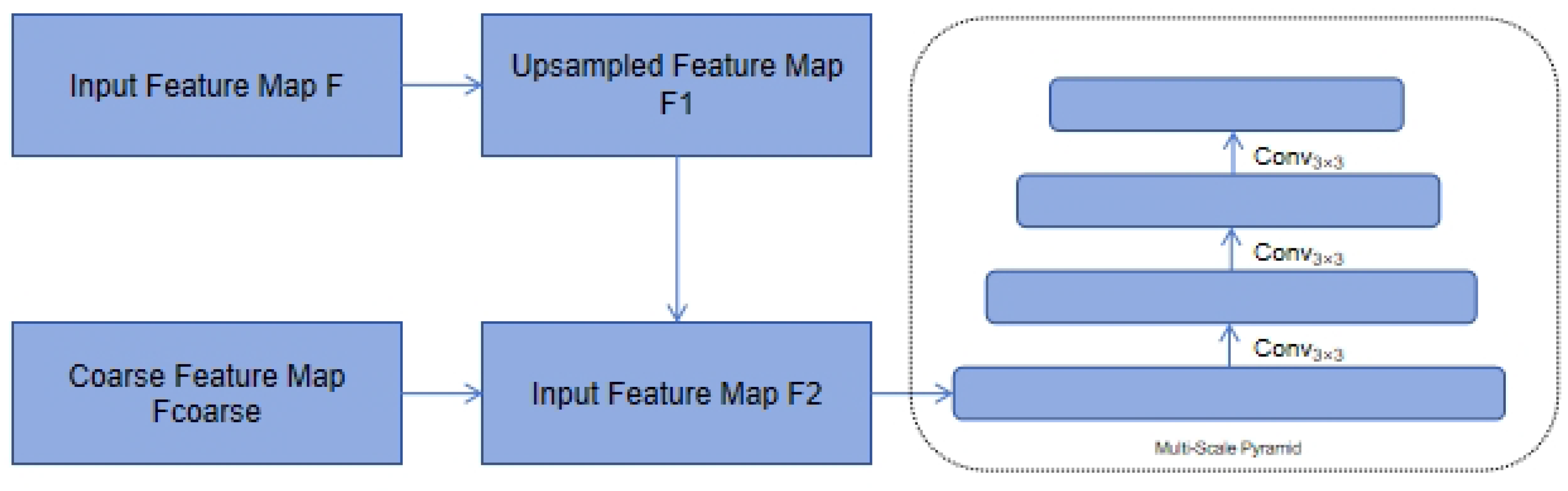
After upsampling, the feature map is further processed with a convolution. The convolution operation is defined as Equation (9).
As shown in Equation (8), the feature map is upsampled using bilinear interpolation. Then, as described in Equation (9), the upsampled feature map undergoes a convolution operation.
For the multi-scale encoder, we only downsample the coarsest feature in the multi-scale encoder features to build the feature pyramid. For the multi-scale encoder output, assuming the coarsest feature map is , we construct the feature pyramid through downsampling operations:
Start with the coarsest feature map . The initial feature map is given.
Next, apply a convolution with stride 2 to the feature map to downsample it. This downsampling operation can be expressed.
Repeat this downsampling step as necessary to construct the feature pyramid.
As shown in Equation (10), we start with the coarsest feature map . Then, as described in Equation (11), a downsampling operation is applied to the feature map.
The Multi-Scale Adapter is crucial for object detection tasks, as it transforms single-scale or multi-scale features into a multi-scale feature pyramid. This enhances the ability of auxiliary feature extractors to meet their needs, improving the effectiveness and efficiency of the object detection system. The adapter achieves this through bilinear interpolation and convolution operations or downsampling the coarsest feature map, constructing multi-level feature representations. In summary, the Multi-Scale Adapter greatly facilitates performance optimization and training convergence of object detection models.
3.3. Auxiliary Feature Extractor
In modern object detection frameworks, feature extraction and accurate prediction play crucial roles in achieving high performance. auxiliary feature extractors are introduced to provide additional supervision signals during the training phase, thereby enhancing the learning of features. This section explains the process and significance of using auxiliary feature extractors in our model.
Given the input image I, after passing through the Backbone (including the HWF and Convolutional Neural Network (CNN)) and the Transformer encoder, we obtain the feature map F.
Multi-scale adapter processes the feature map F, generating multi-scale features .
Each auxiliary feature extractor processes the multi-scale features, generating classification predictions and regression predictions .
Where k denotes the k-th auxiliary feature extractor.
The use of auxiliary feature extractors enhances feature learning by providing additional supervision signals during training. Unlike traditional data augmentation, which increases data diversity through geometric and color transformations, auxiliary feature extractors generate extra labels and features to improve the model’s encoding and decoding abilities. This method enhances feature-level diversity and information content, leading to improved model performance and generalization.
We use three different auxiliary feature extractors in our experiments:ATSS, YOLOv3 and Faster-RCNN. ATSS (Adaptive Training Sample Selection) [34] bridges the gap between anchor-based and anchor-free detection methods, offering adaptability and robustness in various scenarios. YOLOv3 [35] is a single-stage detector that predicts multiple object bounding boxes and categories in a single forward pass, excelling in computational efficiency. Faster-RCNN [36] is a region-based convolutional neural network that combines a Region Proposal Network (RPN) with a Fast R-CNN detector. It provides higher detection accuracy but requires more computational resources.
3.4. Loss Function and Optimization
In deep learning, the loss function and optimization are central to the training process. The loss function quantifies the discrepancy between the model’s predictions and the ground truth, while optimization methods are used to adjust the model parameters to minimize this discrepancy. In this section, we discuss the loss functions used in our model, the total loss function, and the optimization process.
The loss function in our model consists of two main components: classification loss and regression loss. These losses are calculated separately for each auxiliary feature extractor. The classification loss measures the difference between the predicted class probabilities and the true class labels, while the regression loss measures the difference between the predicted bounding box coordinates and the ground-truth coordinates.
In object detection, the classification loss measures the difference between the predicted class and the ground truth class label, typically calculated using cross-entropy loss. The formula is as Equation (15).
where is the predicted class output from the k-th auxiliary feature extractor, and is the ground truth class label.
The regression loss measures the difference between the predicted bounding box and the ground truth bounding box, typically computed using smooth L1 loss. The formula is as Equation (16).
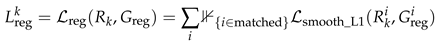 where is the regression output (e.g., bounding box coordinates) from the k-th auxiliary feature extractor, is the ground truth bounding box coordinates, and
  is an indicator function that checks whether the predicted and ground truth boxes are matched.
is an indicator function that checks whether the predicted and ground truth boxes are matched.Similarly, the regression loss is computed as Equation (18).
Where and are the predicted class and bounding box coordinates, and and are the ground truth class labels and bounding box coordinates.
The total loss function is the weighted sum of the classification and regression losses from all auxiliary feature extractors. It is formulated as Equation (19).
Here, and are the weighting coefficients, which balance the contributions of the classification and regression losses.
To minimize the total loss function , we use an optimization algorithm to update the model parameters during training. We employ the Adam optimizer, which combines the benefits of both adaptive learning rates and momentum, making it effective for training deep networks. The optimization process aims to minimize the total loss function by adjusting the model’s parameters iteratively.
The design of the loss function significantly impacts the optimization process. By balancing the classification and regression losses appropriately, we ensure that the model is not biased toward one task over the other. The loss function guides the optimization process toward finding the best model parameters that minimize the prediction errors for both classification and bounding box regression tasks. Furthermore, the auxiliary feature extractors help regularize the model by providing additional supervision signals, which enhances the optimization process and prevents overfitting.
In summary, the loss function and optimization play a crucial role in training our model, ensuring that it effectively learns to perform both classification and regression tasks while generalizing well to unseen data.
4. Experiments
4.1. Dataset and Details
In this study, we utilized the HRSiD (High-resolution Synthetic Aperture Radar Ship Detection) [37] dataset, which is specifically designed for ship detection tasks using high-resolution Synthetic Aperture Radar (SAR) images. The HRSiD dataset contains a large number of high-resolution SAR images captured under various environmental conditions, aimed at evaluating the performance of ship detection algorithms in complex backgrounds. The dataset includes data from multiple voyages, covering a range of weather conditions, sea states, and different types of ships. Each image is meticulously annotated with detailed information, such as ship categories and locations, providing comprehensive support for model training and performance evaluation. In this research, we used the HRSiD dataset for both model training and testing, with the goal of validating the effectiveness and robustness of our proposed method in ship detection tasks.
To better illustrate the characteristics of the HRSiD dataset, we present two example images. Figure 3a shows a high-resolution SAR image of a ship under calm sea conditions, while Figure 3b depicts a ship in a more complex maritime environment with rough sea states. These images highlight the challenges of ship detection in SAR imagery, including varying ship types, sea states, and environmental conditions.
Our experiments also use two-dimensional spectrograms generated from radio waves through a Short-Time Fourier Transform (STFT). These serve as primary input for our model, with the horizontal axis representing signal frequency and the vertical axis denoting time. The signal is visually depicted as a rectangular block within the spectrogram for clarity. We also utilize the Spectral color mapping scheme to enhance diagram efficacy. Specific parameter settings tailored for our dataset are as shown in Table 1.
In our experiments, the 10 modulation modes are considered separately. The signal can be divided into two types: unaliased and aliased, as shown in “Figure 4a”.“Figure 4a” is a simple pattern of radio with no time and frequency aliasing, while “Figure 4b” is a complex pattern with time or frequency aliasing.
We analyzed signals with random durations determined by the DataBitLength parameter, which was varied between minimum and maximum bit lengths for each modulation type. The minimum bit length ranged from 20-200, and the maximum bit length ranged from 400-3000. Storage duration was calculated based on the number of samples and sampling rate to allow for visualization as 512x512 spectrograms.
We conducted extensive trials to compare our model with other successful detectors. All experiments were carried out on a GeForce RTX 3070 GPU. We trained all detectors using the SGD optimizer, with a momentum of 0.937 and a weight decay of 0.00001.
In our experiments, we adopted ATSS [34] as auxiliary feature extractors. We set the number of learnable object queries to 300 and the hyperparameters to the default values of . Here, and control the loss function.
The selection of the appropriate auxiliary feature extractor is crucial for achieving both high detection accuracy and computational efficiency. While Faster R-CNN offers higher accuracy, it is more computationally demanding. In contrast, single-stage detectors like YOLO and SSD are typically more efficient, making them ideal for real-time detection tasks. The choice of auxiliary feature extractor should also take into account specific application scenarios and dataset characteristics to optimize model performance and applicability.
4.2. Comparative Experiments
Under the same experimental configuration, we compared our model with other DETR-based models.All results are reproduced using mmdetection.
Table 2 presents the results of the comparative experiments conducted on the HRSID dataset, evaluating different methods using mAP50 and mAP (mAP50:95). The results demonstrate that our proposed method achieves a mAP of 0.682, surpassing all other methods, including the previous state-of-the-art CS3Net, which achieved a mAP of 0.66. Additionally, our method achieves competitive performance in terms of mAP50, reaching 0.902, which is comparable to CS3Net (0.912) and Yue et al. (0.911).
Compared to lightweight models such as YOLOv6n, YOLOv7-tiny, and YOLOv8n, our method not only outperforms them in mAP but also achieves a favorable trade-off between accuracy and model complexity. Furthermore, while the CS3Net and Yue et al. methods achieve high mAP50 scores, they fall short in terms of mAP, indicating the robustness of our method across varying IoU thresholds. These results highlight the superior performance of our approach in detecting small and challenging objects in the HRSID dataset.
The comparative experimental results, as presented in Table 3, highlight the effectiveness of the proposed Refined Deformable-DETR model in comparison to other DETR-based methods and popular object detection frameworks. The Refined Deformable-DETR achieves the highest performance across all evaluation metrics, with the best results obtained after 36 epochs of training. Specifically, it achieves an of 0.540, an of 0.804, and an of 0.586, which significantly surpasses the results of the baseline Deformable-DETR and other DETR variants.
Compared to the original Deformable-DETR, the refined version demonstrates substantial improvements across all metrics, with an increase of 0.283 in , 0.399 in , and 0.313 in . Furthermore, the proposed model excels in detecting small and medium objects, achieving and , indicating its robustness across different object scales. These improvements are attributed to the introduction of the and the refined architecture, which enhance the feature representation and learning capacity of the model.
Overall, the Refined Deformable-DETR achieves state-of-the-art performance, with notable improvements in accuracy, scalability, and training efficiency, validating its effectiveness in object detection tasks under challenging conditions.
To further analyze the model’s performance across different modulation schemes, we present the confusion matrix in Figure 5. From the confusion matrix, we observe that the model performs exceptionally well on certain classes, such as GMSK and 64QAM, with classification accuracies of 66% and 89%, respectively. This indicates that these modulation schemes have distinct characteristics, making them easier for the model to classify correctly.
The confusion matrix analysis reveals the model’s performance across different modulation schemes. Although the model performs well on certain signals, it struggles to distinguish between similar modulation types. Future work could introduce more advanced feature extractors or utilize higher-level supervisory signals to improve classification performance.
4.3. Ablation Study
In this section, we compared the impact of different auxiliary feature extractors on model performance. We selected YOLOv3 [35], Faster-RCNN [36] and ATSS [34] as auxiliary feature extractors, and conducted experiments under various configurations.
The results of the ablation study on the HRSID dataset are shown in Table 4. When HWF is enabled, YOLOv3 outperforms the other two extractors with an AP of 0.682 and AP50 of 0.902. Faster-RCNN shows slightly lower performance, with an AP of 0.602 and AP50 of 0.858. ATSS achieves an AP of 0.677 and an AP50 of 0.882. All extractors show a decrease in performance when HWF is disabled, with YOLOv3 maintaining the best performance in both AP and AP50 under the non-HWF configuration.
Table 5 presents the results of the ablation study on the Spectrograms dataset. YOLOv3, with HWF enabled, achieves an AP of 0.540 and an AP50 of 0.804. The performance decreases slightly when HWF is disabled. Faster-RCNN and ATSS also demonstrate similar trends, with ATSS yielding the best performance among the three, reaching an AP of 0.533 and an AP50 of 0.771 when HWF is enabled. For both datasets, disabling HWF leads to a reduction in performance, although the degree of the drop varies between extractors and datasets.
The results from both datasets suggest that the HWF module is particularly effective in scenarios requiring high-precision detections. On the HRSID dataset, which contains diverse targets including medium and large objects, the module provides significant benefits in both AP and AP50. On the Spectrograms dataset, which involves more complex signal patterns, the module still contributes to performance improvements, albeit to a lesser extent.
In conclusion, this ablation study highlights the positive impact of the HWF module on detection performance, demonstrating its ability to enhance feature extraction and improve recognition accuracy across different datasets. While the gains are more prominent on the HRSID dataset, the consistent improvements across datasets underline the utility of the HWF module as a general enhancement for detection tasks.
5. Conclusion
We proposed Refined Deformable-DETR, for SAR target detection and signal modulation recognition. Experimental results demonstrate the outstanding performance of Refined Deformable-DETR. By proposing the half-window filtering technique and the Auxiliary Feature Extractor, Refined Deformable-DETR enhances detection performance, particularly for small, medium, and large targets. In the context of SAR target detection, the model effectively handles complex background environments, improving detection accuracy in cluttered or noisy scenarios. Moreover, the model shows robust performance in signal modulation recognition, further validating its effectiveness in electromagnetic environments. Future work will focus on optimizing the training process to enhance efficiency and exploring additional application scenarios to achieve more efficient and accurate signal detection and recognition, particularly in SAR-based tasks.
Author Contributions
Zhenghao Li was responsible for methodology, software development, formal analysis, and drafting the original manuscript. Xin Zhou contributed to the conceptualization, investigation, resource acquisition, and reviewing and editing of the manuscript. Both authors collaborated on the design and implementation of the research and approved the final version of the manuscript for submission.
Conflicts of Interest
The authors declare no conflicts of interest.
References
- Chen, C.; He, C.; Hu, C.; Pei, H.; Jiao, L. MSARN: A Deep Neural Network Based on an Adaptive Recalibration Mechanism for Multiscale and Arbitrary-Oriented SAR Ship Detection. IEEE Access 2019, p. 159262–159283. [CrossRef]
- Wang, Y.; Wang, C.; Zhang, H. Ship Classification in High-Resolution SAR Images Using Deep Learning of Small Datasets. Sensors 2018, p. 2929. [CrossRef]
- Zhao, Z.Q.; Zheng, P.; Xu, S.T.; Wu, X. Object Detection with Deep Learning: A Review. IEEE Transactions on Neural Networks and Learning Systems 2019, p. 3212–3232. [CrossRef]
- O’Shea, T.J.; Corgan, J.; Clancy, T.C. Convolutional Radio Modulation Recognition Networks. In Proceedings of the Proceedings of the International Conference on Engineering Applications of Neural Networks, 2016, pp. 213–226.
- Sturmel, N.; Daudet, L.; et al. Signal Reconstruction from STFT Magnitude: A State of the Art. In Proceedings of the Proceedings of the International Conference on Digital Audio Effects (DAFx), 2011, pp. 375–386.
- Girshick, R. Fast R-CNN. In Proceedings of the 2015 IEEE International Conference on Computer Vision (ICCV), Dec 2015. [CrossRef]
- Krasner, N. Optimal Detection of Digitally Modulated Signals. IEEE Transactions on Communications 1982, 30, 885–895.
- Rahman, M.H.; Sejan, M.A.S.; Aziz, M.A.; Baik, J.I.; Kim, D.S.; Song, H.K. Deep Learning Based Improved Cascaded Channel Estimation and Signal Detection for Reconfigurable Intelligent Surfaces-Assisted MU-MISO Systems. IEEE Transactions on Green Communications and Networking 2023, 7, 1515–1527. [CrossRef]
- Vaswani, A.; Shazeer, N.; Parmar, N.; Uszkoreit, J.; Jones, L.; Gomez, A.N.; Kaiser, L.; Polosukhin, I. Attention Is All You Need. In Proceedings of the Proceedings of the 31st International Conference on Neural Information Processing Systems (NeurIPS), Long Beach, CA, USA, 2017; pp. 5998–6008.
- Carion, N.; Massa, F.; Synnaeve, G.; Usunier, N.; Kirillov, A.; Zagoruyko, S. End-to-End Object Detection with Transformers. In Proceedings of the Proceedings of the European Conference on Computer Vision (ECCV), 2020, pp. 213–229.
- Ren, S.; He, K.; Girshick, R.; Sun, J. Faster r-cnn: Towards real-time object detection with region proposal networks. Advances in neural information processing systems 2015, 28.
- Girshick, R.; Donahue, J.; Darrell, T.; Malik, J. Rich Feature Hierarchies for Accurate Object Detection and Semantic Segmentation. In Proceedings of the 2014 IEEE Conference on Computer Vision and Pattern Recognition, Jun 2014. [CrossRef]
- Zhu, X.; Su, W.; Lu, L.; Li, B.; Wang, X.; Dai, J. Deformable detr: Deformable transformers for end-to-end object detection. arXiv preprint arXiv:2010.04159 2020.
- Meng, D.; Chen, X.; Fan, Z.; Zeng, G.; Li, H.; Yuan, Y.; Sun, L.; Wang, J. Conditional detr for fast training convergence. In Proceedings of the Proceedings of the IEEE/CVF international conference on computer vision, 2021, pp. 3651–3660.
- Liu, S.; Li, F.; Zhang, H.; Yang, X.; Qi, X.; Su, H.; Zhu, J.; Zhang, L. Dab-detr: Dynamic anchor boxes are better queries for detr. arXiv preprint arXiv:2201.12329 2022.
- Ding, S.G.; Nie, X.L.; Qiao, H.; Zhang, B. Online classification for SAR target recognition based on SVM and approximate convex hull vertices selection. National Key Laboratory of Management and Control for Complex Systems 2014, pp. 1473–1478.
- Yu, G.; Ying, X. Architecture design of deep convolutional neural network for SAR target recognition. Journal of Image and Graphics 2018.
- Kang, M.; Leng, X.; Lin, Z.; Ji, K. A modified faster R-CNN based on CFAR algorithm for SAR ship detection. IEEE 2017.
- Redmon, J.; Divvala, S.; Girshick, R.; Farhadi, A. You Only Look Once: Unified, Real-Time Object Detection. In Proceedings of the 2016 IEEE Conference on Computer Vision and Pattern Recognition (CVPR), Jun 2016. [CrossRef]
- Oh, J.; Kim, M. PeaceGAN: A GAN-Based Multi-Task Learning Method for SAR Target Image Generation with a Pose Estimator and an Auxiliary Classifier. Remote Sensing 2021, p. 3939. [CrossRef]
- Lu, D.; Cao, L.; Liu, H. Few-Shot Learning Neural Network for SAR Target Recognition. In Proceedings of the 2019 6th Asia-Pacific Conference on Synthetic Aperture Radar (APSAR), Nov 2019, p. 1–4. [CrossRef]
- Zhu, X.; Mori, H. Data augmentation using style transfer in SAR automatic target classification. In Proceedings of the Artificial Intelligence and Machine Learning in Defense Applications III, Sep 2021, p. 12. [CrossRef]
- Gong, Y.; Sbalzarini, I.F. Curvature Filters Efficiently Reduce Certain Variational Energies. IEEE Transactions on Image Processing 2017, p. 1786–1798. [CrossRef]
- Ibrahim, M.; Chen, K.; Brito-Loeza, C. A novel variational model for image registration using Gaussian curvature. Geometry, Imaging and Computing 2014, 1, 417–446. [CrossRef]
- Zhu, H.; Shu, H.; Zhou, J.; Bao, X.; Luo, L. Bayesian algorithms for PET image reconstruction with mean curvature and Gauss curvature diffusion regularizations. Computers in Biology and Medicine 2007, 37, 793–804. [CrossRef]
- Rudin, L.I.; Osher, S.; Fatemi, E. Nonlinear total variation based noise removal algorithms. Physica D: Nonlinear Phenomena 1992, p. 259–268. [CrossRef]
- He, K.; Zhang, X.; Ren, S.; Sun, J. Deep Residual Learning for Image Recognition. In Proceedings of the 2016 IEEE Conference on Computer Vision and Pattern Recognition (CVPR), Jun 2016. [CrossRef]
- Caruana, R. Multitask Learning. Machine Learning 1997, p. 41–75. [CrossRef]
- Radford, A.; Kim, J.; Hallacy, C.; Ramesh, A.; Goh, G.; Agarwal, S.; Sastry, G.; Amanda, A.; Mishkin, P.; Clark, J.; et al. Learning Transferable Visual Models From Natural Language Supervision. Cornell University - arXiv,Cornell University - arXiv 2021.
- Isola, P.; Zhu, J.Y.; Zhou, T.; Efros, A.A. Image-to-Image Translation with Conditional Adversarial Networks. In Proceedings of the 2017 IEEE Conference on Computer Vision and Pattern Recognition (CVPR), Jul 2017. [CrossRef]
- Jaderberg, M.; Mnih, V.; Czarnecki, W.; Schaul, T.; Leibo, J.; Silver, D.; Kavukcuoglu, K. Reinforcement Learning with Unsupervised Auxiliary Tasks. arXiv: Learning,arXiv: Learning 2016.
- Zong, Z.; Song, G.; Liu, Y. DETRs with Collaborative Hybrid Assignments Training 2022.
- Zhang, J.; Tian, G.; Mu, Y.; Fan, W. Supervised deep learning with auxiliary networks. In Proceedings of the Proceedings of the 20th ACM SIGKDD international conference on Knowledge discovery and data mining, Aug 2014. [CrossRef]
- Zhang, S.; Chi, C.; Yao, Y.; Lei, Z.; Li, S.Z. Bridging the Gap Between Anchor-based and Anchor-free Detection via Adaptive Training Sample Selection. In Proceedings of the 2020 IEEE/CVF Conference on Computer Vision and Pattern Recognition (CVPR), Jun 2020. [CrossRef]
- Redmon, J.; Farhadi, A. YOLOv3: An Incremental Improvement. arXiv: Computer Vision and Pattern Recognition,arXiv: Computer Vision and Pattern Recognition 2018.
- Ren, S.; He, K.; Girshick, R.; Sun, J. Faster R-CNN: Towards Real-Time Object Detection with Region Proposal Networks. IEEE Transactions on Pattern Analysis and Machine Intelligence 2017, p. 1137–1149. [CrossRef]
- Wei, S.; Zeng, X.; Qu, Q.; Wang, M.; Su, H.; Shi, J. HRSID: A High-Resolution SAR Images Dataset for Ship Detection and Instance Segmentation. IEEE Access 2020, p. 120234–120254. [CrossRef]
- Yue, T.; Zhang, Y.; Liu, P.; Xu, Y.; Yu, C. A Generating-Anchor Network for Small Ship Detection in SAR Images. IEEE Journal of Selected Topics in Applied Earth Observations and Remote Sensing 2022, p. 7665–7676. [CrossRef]
- Gao, F.; Cai, C.; Tang, W.; He, Y. A compact and high-efficiency anchor-free network based on contour key points for SAR ship detection. IEEE Geoscience and Remote Sensing Letters 2024.
- Bai, L.; Yao, C.; Ye, Z.; Xue, D.; Lin, X.; Hui, M. Feature Enhancement Pyramid and Shallow Feature Reconstruction Network for SAR Ship Detection.
- Zhang, T.; Zhang, X.; Liu, C.; Shi, J.; Wei, S.; Ahmad, I.; Zhan, X.; Zhou, Y.; Pan, D.; Li, J.; et al. Balance learning for ship detection from synthetic aperture radar remote sensing imagery. ISPRS Journal of Photogrammetry and Remote Sensing 2021, p. 190–207. [CrossRef]
- Bai, L.; Yao, C.; Ye, Z.; Xue, D.; Lin, X.; Hui, M. A Novel Anchor-Free Detector Using Global Context-Guide Feature Balance Pyramid and United Attention for SAR Ship Detection. IEEE Geoscience and Remote Sensing Letters 2023, p. 1–5. [CrossRef]
- Chen, C.; Zeng, W.; Zhang, X.; Zhou, Y. CS n Net: A Remote Sensing Detection Network Breaking the Second-Order Limitation of Transformers with Recursive Convolutions.
Figure 1.
Overview of the proposed Refined Deformable-DETR model architecture for SAR target detection and radio signal detection. The model processes input SAR image and spectrograms through HWF and a Transformer encoder, followed by multi-scale feature adaptation and auxiliary feature extraction to generate final classification and regression predictions.
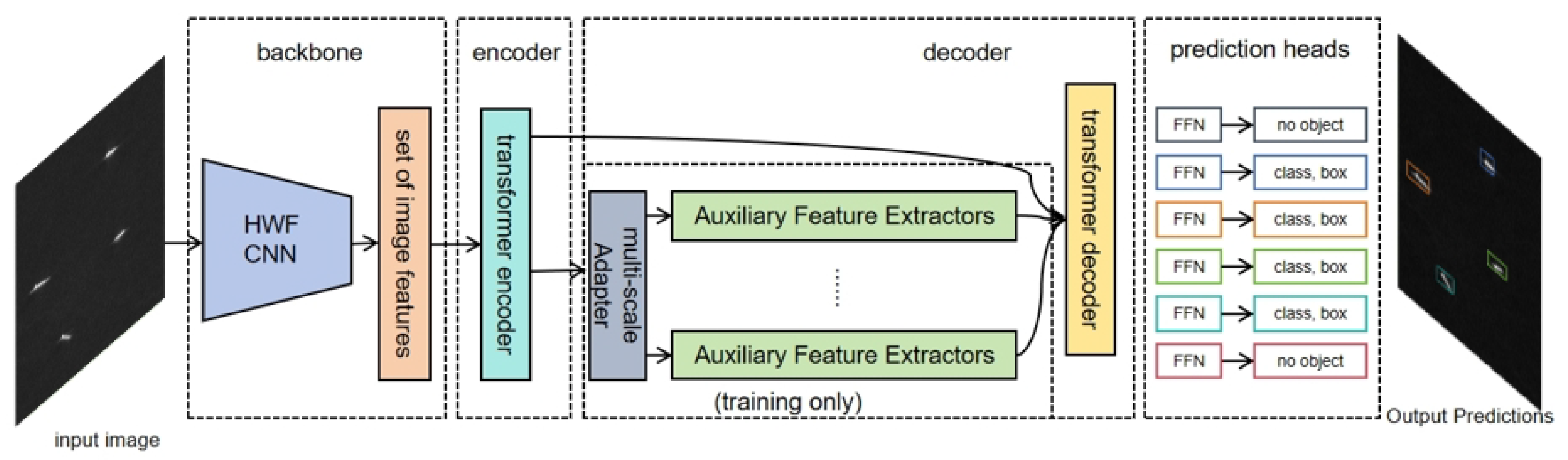
Figure 3.
Example SAR images from the HRSiD dataset illustrating ship detection in different sea states.
Figure 3.
Example SAR images from the HRSiD dataset illustrating ship detection in different sea states.
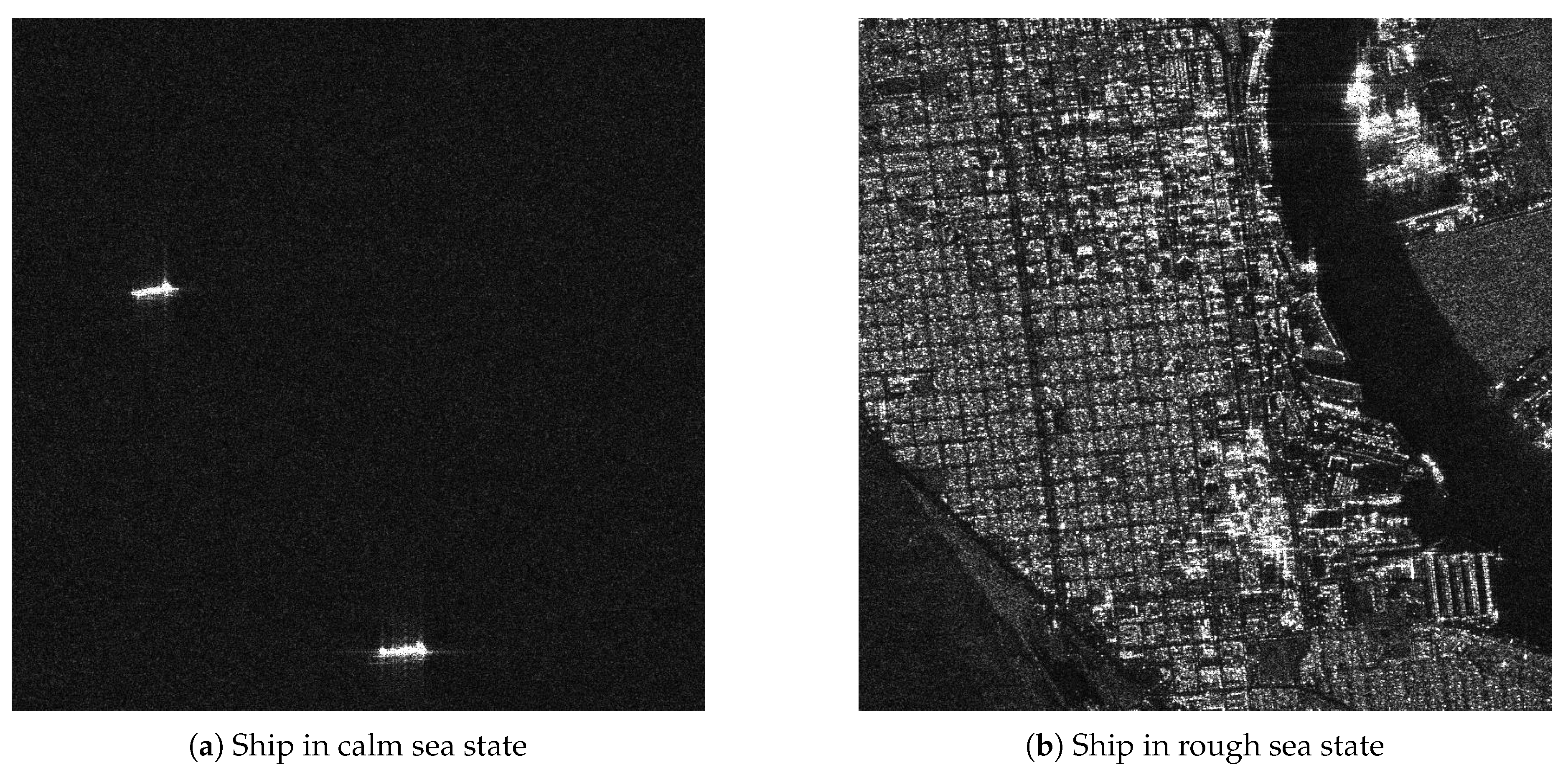
Figure 4.
Visualization of spectrograms of radio signal.
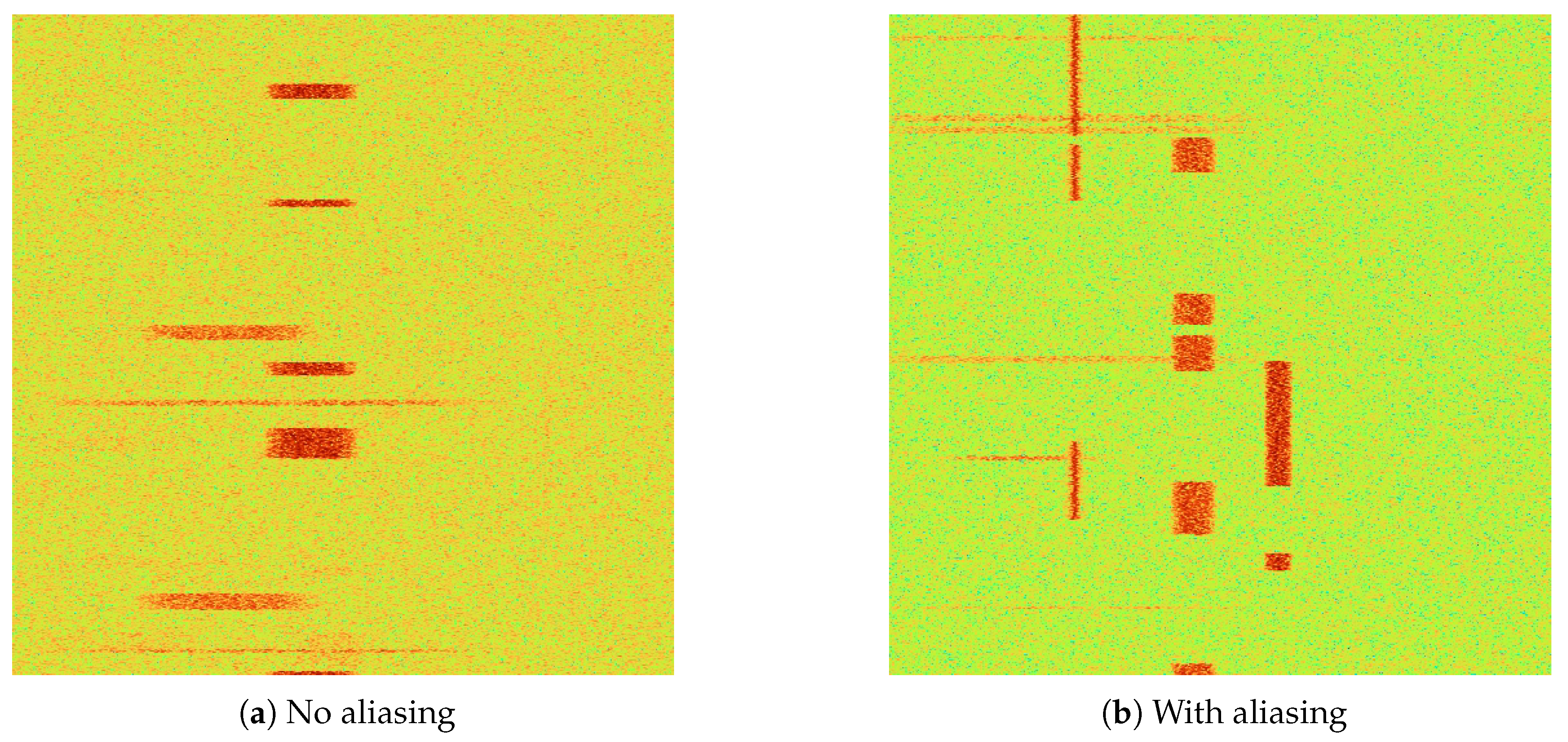
Figure 5.
Normalized confusion matrix showing the classification performance of the model for each modulation type. The diagonal values represent correct classifications, while the off-diagonal values represent misclassifications.
Figure 5.
Normalized confusion matrix showing the classification performance of the model for each modulation type. The diagonal values represent correct classifications, while the off-diagonal values represent misclassifications.
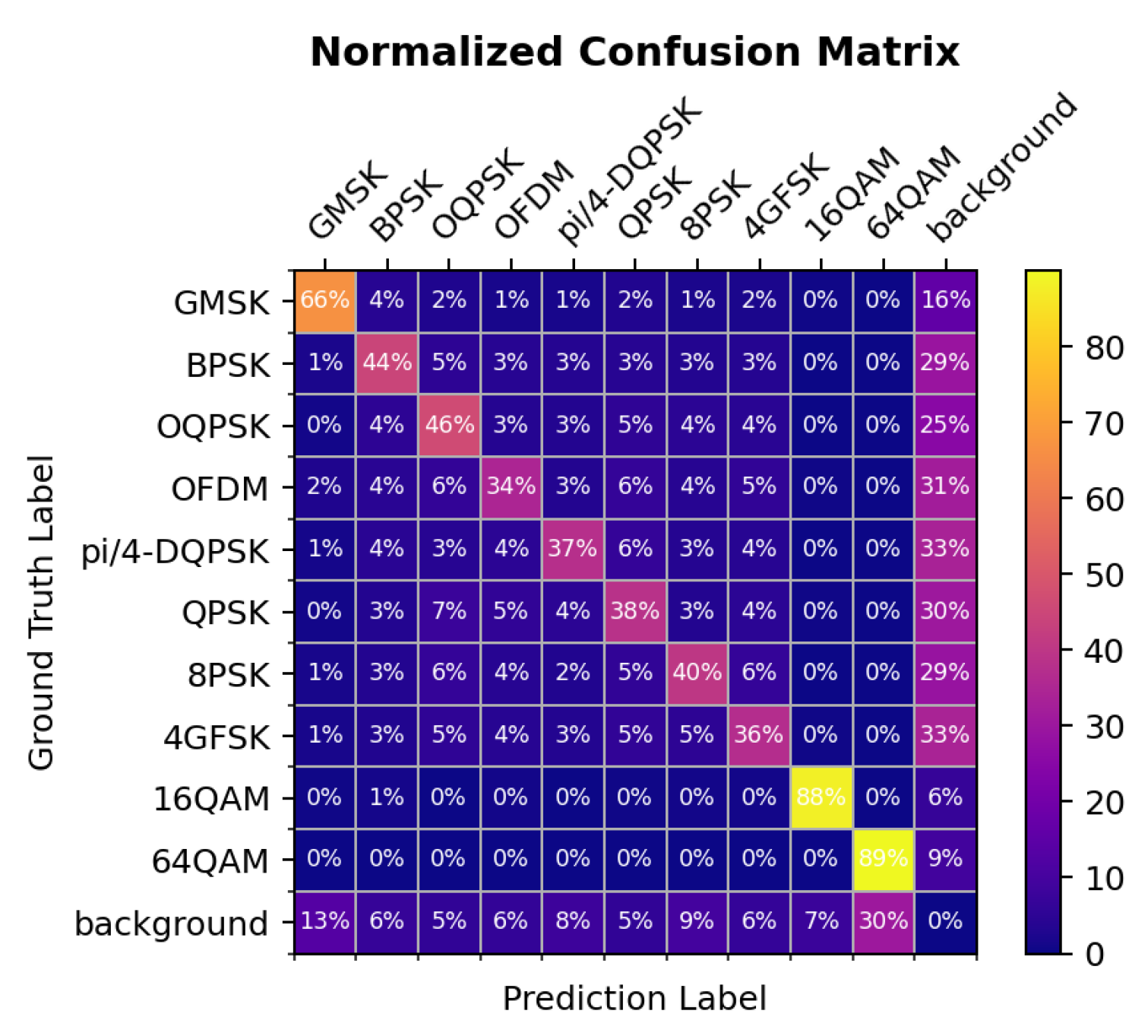

Table 1.
Dataset Parameters.
| Parameter | Value |
|---|---|
| Total sample | 12500 |
| Sampling rate | 1024kHz |
| Bandwidth | [10, 20, 50, 100, 150]Hz |
| Signal Power | [0.1, 0.125, 0.25, 0.5, 1, 2, 4, 8, 10, 100] |
| Modulation methods | BPSK, QPSK, 8PSK, OQPSK, 16PSK, 16QAM, 64QAM, 256QAM, 2FSK, 4FSK |
| Noise Power | 1 |
| Size of spectrograms | (512, 512) |
| Ratio of dataset | train : validation : test = 8 : 1 : 1 |
Table 2.
Comparison Experiments on HRSID.
| Method | mAP50 | mAP |
|---|---|---|
| Faster RCNN | 0.720 | 0.465 |
| RetinaNet | 0.789 | 0.536 |
| YOLOv6n | 0.882 | 0.628 |
| YOLOv7-tiny | 0.854 | 0.572 |
| YOLOv8n | 0.911 | 0.669 |
| YOLOv11n | 0.897 | 0.658 |
| Yue et al. [38]* | 0.911 | 0.665 |
| CPoints-Net [39]* | 0.905 | - |
| FEPS-Net [40]* | 0.907 | 0.657 |
| BL-Net [41]* | 0.867 | - |
| FBUA-Net [42]* | 0.903 | - |
| CS3Net [43]* | 0.912 | 0.66 |
| Refined Deformable-DETR | 0.902 | 0.682 |
Denotes data obtained from their papers
Table 3.
Comparison of Different Methods on Spectrograms Dataset.
| Method | Backbone | AP | AP50 | AP75 | APS | APM | APL |
|---|---|---|---|---|---|---|---|
| CenterNet | Resnet18 | 0.169 | 0.299 | 0.160 | 0.122 | 0.301 | 0.417 |
| Faster-Rcnn | Resnet50 | 0.139 | 0.164 | 0.156 | 0.037 | 0.417 | 0.551 |
| YOLOv3 | Darknet | 0.004 | 0.011 | 0.003 | 0.001 | 0.012 | 0.102 |
| CornerNet | HourglassNet | 0.207 | 0.315 | 0.217 | 0.162 | 0.335 | 0.421 |
| DETR | Resnet18 | 0.266 | 0.513 | 0.238 | 0.170 | 0.503 | 0.780 |
| DETR | Resnet50 | 0.086 | 0.178 | 0.076 | 0.051 | 0.201 | 0.770 |
| Deformable-DETR | Resnet50 | 0.257 | 0.405 | 0.273 | 0.225 | 0.372 | 0.997 |
| DAB-DETR | Resnet50 | 0.211 | 0.391 | 0.195 | 0.170 | 0.360 | 0.898 |
| DAB-DETR | Resnet50 | 0.228 | 0.422 | 0.213 | 0.171 | 0.431 | 0.915 |
| Conditional-DETR | Resnet50 | 0.112 | 0.223 | 0.093 | 0.078 | 0.221 | 0.788 |
| Refined Deformable-DETR | Resnet50 | 0.540 | 0.804 | 0.586 | 0.462 | 0.791 | 0.986 |
Table 4.
Comparison of Auxiliary Extractors on HRSID.
| Auxiliary Feature Extractor | HWF | AP | AP50 |
|---|---|---|---|
| YOLOv3 based AFE | ✓ | 0.682 | 0.902 |
| × | 0.619 | 0.887 | |
| Faster-RCNN based AFE | ✓ | 0.602 | 0.858 |
| × | 0.587 | 0.822 | |
| ATSS based AFE | ✓ | 0.677 | 0.882 |
| × | 0.652 | 0.837 |
Table 5.
Comparison of Auxiliary Extractors on Spectrograms Dataset.
| Auxiliary Feature Extractor | HWF | AP | AP50 |
|---|---|---|---|
| YOLOv3 based AFE | ✓ | 0.540 | 0.804 |
| × | 0.525 | 0.794 | |
| Faster-RCNN based AFE | ✓ | 0.527 | 0.782 |
| × | 0.499 | 0.664 | |
| ATSS based AFE | ✓ | 0.533 | 0.771 |
| × | 0.510 | 0.752 |
Disclaimer/Publisher’s Note: The statements, opinions and data contained in all publications are solely those of the individual author(s) and contributor(s) and not of MDPI and/or the editor(s). MDPI and/or the editor(s) disclaim responsibility for any injury to people or property resulting from any ideas, methods, instructions or products referred to in the content. |
© 2025 by the authors. Licensee MDPI, Basel, Switzerland. This article is an open access article distributed under the terms and conditions of the Creative Commons Attribution (CC BY) license (http://creativecommons.org/licenses/by/4.0/).
Copyright: This open access article is published under a Creative Commons CC BY 4.0 license, which permit the free download, distribution, and reuse, provided that the author and preprint are cited in any reuse.


