
Submitted:
20 January 2025
Posted:
21 January 2025
You are already at the latest version
Abstract
The increase in the penetration rate of new energy in the power grid has led to a serious lack of flexibility in the power system during certain periods. In order to solve the problem that the existing methods for dealing with power system flexibility and supply and demand uncertainty are too conservative or risky, a data-driven distributed robust optimization dispatching model is proposed. Firstly, considering the temporal and spatial correlation of wind and photovoltaic power output, an output set is constructed based on Copula theory. The flexibility demand of the power system is quantified by combining the scenario method and the interval method, and the flexible adjustment factor is introduced to characterize the ability of various resources to participate in flexibility adjustment, and the flexibility supply and demand balance constraint is established. Secondly, considering the flexible supply capacity of demand-side resources such as electric vehicles, a data-driven two-stage distribution robust model is established with the optimal flexibility resource operating cost and grid flexibility deficit penalty cost as the objective function. In order to reduce conservatism, the comprehensive norm is used to constrain its probability distribution, which reduces the probability of extreme situations in flexibility demand. In order to solve the two-stage robust model problem, the zero-sum game idea is used to decouple the model into the main problem and sub-problems, and the column and constraint generation algorithm is used for iterative solution. Finally, the simulation example shows that the proposed model has a positive effect on improving the flexibility margin and economy of the power system compared with the traditional uncertainty model.
Keywords:
Supply and demand balance
; Flexibility
; Data-driven
; Distributed Robust Optimal Scheduling
; Column and constraint generation algorithm
1. Introduction
The rapid development of renewable energy power generation equipment and grid-connected technology has led to the gradual formation of a new type of power system dominated by new energy sources [1,2]. The stochastic volatility of a high proportion of new energy leads to a significant increase in the difficulty of power system operation and scheduling, and it is difficult for traditional flexibility resources, such as conventional units, to effectively meet the dramatically increased flexibility demand of the system. At the same time, the current situation that the power grid is seriously insufficient in local time, makes the demand-side flexibility gradually become the core of the research on power grid scheduling and operation. The demand-side flexibility has gradually become the core of the research on grid scheduling and operation.
Flexibility, as delineated by the International Energy Agency (IEA), represents the capacity of grid resources to address flexibility demands within specified timeframes [3,4]. Understanding and quantifying this demand is pivotal for analyzing the supply-demand equilibrium of flexibility in modern power systems. While several studies have ventured into quantifying flexibility demand [5,6,7], they have largely overlooked the critical role of uncertainty. To address this stochastic nature of net load, some research efforts have employed joint probability distribution functions [8,9,10]. However, these probability-based methodologies are inherently limited by their reliance on predefined probability distributions, which often fail to capture the precise flexibility demand and regulation capacity required in each time period. Additionally, attempts to quantify uncertainty in flexibility demand using an error coefficient based on forecast values, as demonstrated in [11], although a step forward, remain overly simplistic and insufficient to fully grasp the complexity and dynamics of uncertainty in power systems. Thus, there is a pressing need for more sophisticated approaches to accurately quantify and manage flexibility demand, taking into account the multifaceted nature of uncertainty.
In recent years, robust optimization (RO) and stochastic optimization (SO) have been applied to the study of flexibility supply and demand equilibrium under the influence of uncertainties. Literature [12,13] constructs the operational domain of flexibility supply and demand equilibrium through robust and conditional value-at-risk. Literature [14,15] establishes a comprehensive stochastic optimization model by solving the flexibility margin through the multi-scenario method and determining the benchmark value according to the Bernstein polynomial theory. All the above methods have the problem of being too conservative or risky in the portrayal of flexibility supply and demand. The distributionally robust optimization (DRO) model combines the strengths of both models by using uncertain probability densities to describe uncertainty and thus find the probability distribution of the worst-case scenario. Traditionally, DRO optimizes fuzzy sets of probability distributions based on moment information or distance measures such as KL (Kullback-Leibler ) dispersion [16]. The former is usually a non-deterministic polynomial (NP) hard problem that is difficult to solve, requires the type of distribution of uncertainty to be specified in advance, and is too conservative when the sample data are large; the latter has the risk of losing the significance of the probability fuzzy set when the assumption error is large. Based on this, a data-driven DRO has been emphasized [17]. The model characterizes uncertainty by extracting a large number of historical data samples of power system operation and establishing a comprehensive set of paradigm uncertainty probabilities. Decision making is guided by historical data rather than moment information that characterizes the overall performance, which makes full use of the sample data and has the advantages of simple solution and good economic flexibility [18]. At present, data-driven DRO has been initially applied in the fields of site selection and capacity determination [19] and unit combination [20], but there is no research report on flexibility supply and demand optimization scheduling.
Demand-side resources have emerged as viable alternatives to generation-side resources in providing flexibility balancing, offering operational adequacy and economic benefits [21]. Unfortunately, prior research has overlooked the substantial flexibility supply potential of demand-side resources. The majority of studies examining their involvement in power system optimal scheduling have been confined to the narrow focus of “power balance,” treating it as a static process of supply and demand. This narrow perspective fails to account for the dynamic fluctuations in supply and demand across various time scales, thereby underutilizing the regulatory potential of demand-side flexibility resources. As the operational paradigm of power systems evolves from the traditional one-way model of power supply matching load to a more sophisticated two-way model encompassing source-network-load-storage coordination and interaction, grid scheduling must adapt. It must harness the full spectrum of demand-side resources to achieve “flexibility balance,” ensuring that the system can meet the flexibility demands of each period effectively [22,23]. This evolution underscores the urgency for research that fully integrates and leverages the flexibility capabilities of demand-side resources.
In addition, the existing supply and demand flexibility studies rarely consider the correlation of wind and light outputs, and the traditional correlation analysis method is difficult to effectively reflect the complementary characteristics of new energy outputs, resulting in the inaccurate description of the set of outputs [24]. Based on the above problems, this paper establishes a data-driven distribution robust optimization scheduling model considering flexibility supply and demand balance, and the main work is as follows:
1) The Copula theory is applied to construct the scenariory spatio-temporal correlation output set, and the flexibility demand is quantified by combining the scenario method and the interval method;
2) Considering the flexibility supply capacity of demand-side resources such as electric vehicles, the effectiveness of the model is verified by comparing multiple flexibility regulation methods;
3) The proposed data-driven DRO model can effectively control the robustness of grid dispatch flexibility and economy, and the superiority of the model is verified by comparing with the existing uncertainty algorithms.
2. Power System Supply and Demand Flexibility and Quantitative Model
As a supplement to the abundance, the flexibility of the power system studies the fluctuation of power under a certain time scale. The dual fluctuation of source and load requires the use of flexible resources to match. If the system is not flexible enough, there will be risks of wind curtailment and load shedding.
To quantify the flexibility of the power system, it is necessary to determine the flexibility demand and the flexibility supply capacity of the flexibility resources respectively. Considering the time scale characteristics, directionality and state dependence of flexibility, the explanation is given from the perspectives of flexibility demand, flexibility supply and flexibility balance.
2.1. Quantification of Flexibility Requirements Considering Spatiotemporal Correlation and Uncertainty
2.1.1. Wind and Photovoltaic Power Generation based on Copula Theory
Copula theory states that the joint probability distribution function can be decomposed into the product of the marginal distribution function and the Copula function. Compared with the traditional simple linear correlation analysis, Copula theory can describe the complex and nonlinear correlation between different random variables. The selection of Copula function is related to the accuracy of the wind and photovoltaic power output set. Considering the complementary characteristics between wind and photovoltaic power output, the Frank-Copula function is selected for description [26]. The specific steps are as follows:
1) The wind power output probability density fW, t(xW, t), distribution function FW, t(xW, t), and photovoltaic output probability density fPV,t(xPV, t), distribution function FPV, t(xPV, t) were calculated based on the historical sample data.
2) The Copula function is constructed to obtain the joint probability distribution H (xPV, xW) of the wind-wind output in each period, and generate a set of random values of the edge distribution function of wind-wind variables with spatiotemporal correlation {uPV, t, uW, t}.
3) The set of random values is inverted by the inverse function, that is, (uPV, t) and (uW, t), and the wind-photovoltaic output set with temporal and spatial dependence is obtained.
2.1.2. Quantifying Flexibility Requirements
The flexibility demand of power grid comes from the random fluctuation of net load obtained from wind-wind load synthesis. In the Data Driven DRO, the need for power system flexibility is quantified using a combination of scenario and interval methods, thereby reducing conservatism while ensuring flexible operation in the day-ahead phase. In this paper, the probabilistic distance based scenario reduction technique is used to obtain typical scenarios from the sample data .
Scenario reduction method based on probability distance is a kind of rapid previous scenario reduction technology, which can find a given number of typical scenarios in a large number of historical sample scenarios, and obtain the occurrence probability of each scenario. Compared with the typical scenario obtained by the clustering method, which is the cluster center, the scenarios obtained by the cutting method are all from the real scenario of the sample, which makes the typical scenario more authentic. The reduction steps are as follows:
Step 1: Determine the cut scenario . Calculate the geometric distance d(s(n),s(m)). between any two scenarios in the history sample S. Considering the probability distance D(n) between scenario probability p(n) and Euclidean distance d, the scenario s(k’) with the smallest sum of probability distance from the remaining scenario s(k*) is selected.
Step 2: Change the probability p(k ') of the scenario closest to the probability s(k ') of the deleted scenario
Step 3: Check whether the number of remaining scenarios meets requirements. Otherwise, return to Step 1.
Taking the load as an example, the load model considering the maximum fluctuation error for the kth scenario can be expressed as:
where: is the predicted value of load at time t in the kth scenario; and are the upper and lower limits of load fluctuation at time t in the kth scenario respectively. εL is the maximum predictive error coefficient of the load.
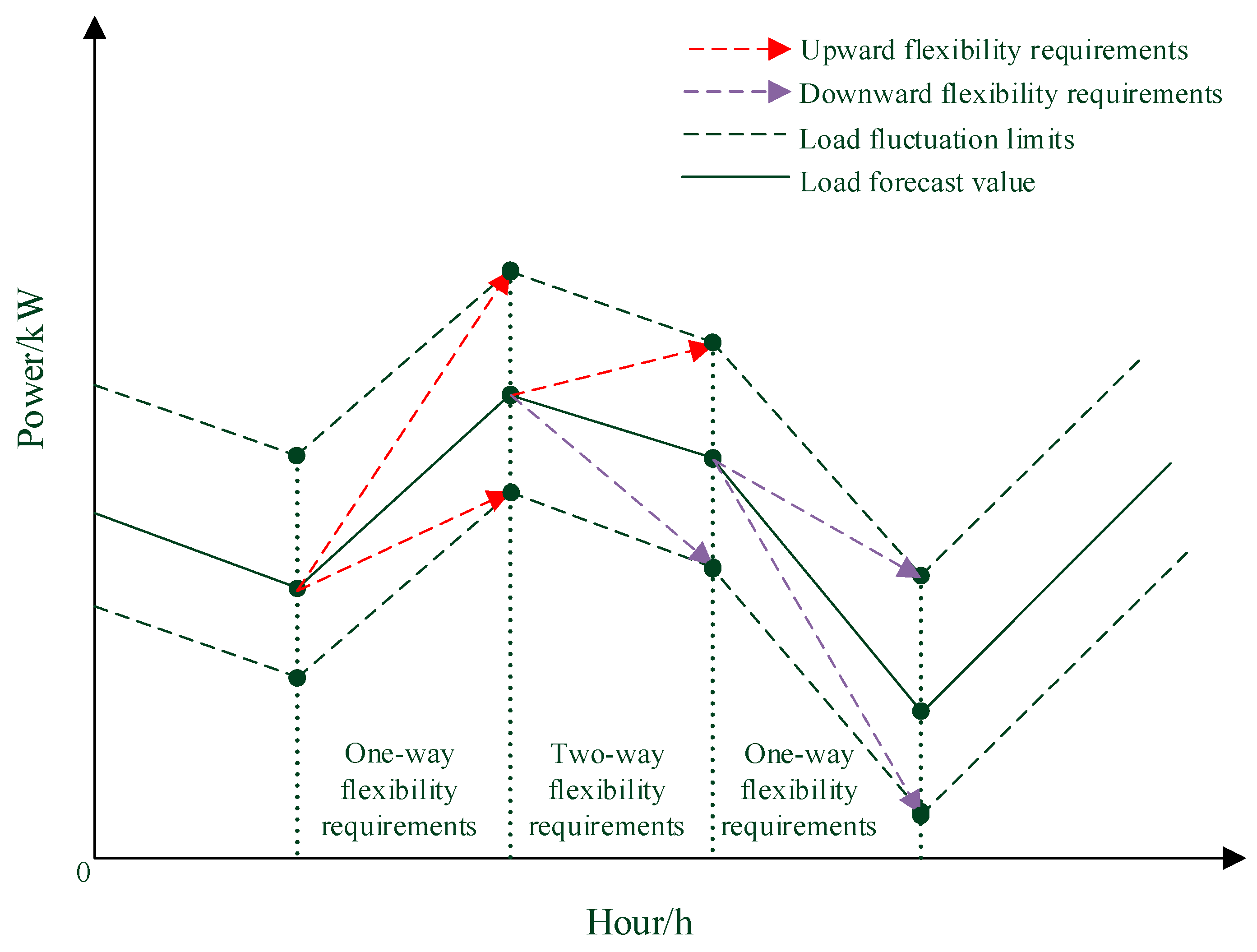
Under the given time scale τ, the flexibility demand for scenario k can be divided into three cases: when ≤, there is only upward flexibility demand; When ≤, there is only downward flexibility demand; When <<, there is bidirectional flexibility demand, that is, there is both upward flexibility demand and downward flexibility demand. Considering the coupling relationship of time, load fluctuation can be represented by the first-order difference of adjacent periods, as shown in equation (4), and the quantification principle of flexibility demand is shown in Figure 2.
Where: andare respectively the upward flexibility demand and downward flexibility demand generated by load at time t in the kth scenario.
Figure 1.
Quantification diagram of flexibility demands .
The process of quantifying the flexibility demand generated by wind power and photovoltaic is similar to that of load, but it should be noted that as a power source its downward fluctuation actually produces an upward flexibility demand, as shown in equations (5) and (6).
where: and is the upper and lower limits of PV at time t in the kth scenario respectively; and are respectively the upper and lower limits of wind power output at time t in the kth scenario.and are the predicted values of PV and wind power output at time t in the kth scenario, respectively. and are respectively the upward and downward flexibility requirements generated by PV at time t in the kth scenario. and are the upward and downward flexibility demands of wind power at time t in the kth scenario, respectively. εPV is the maximum prediction error coefficient of PV; εW is the maximum prediction error coefficient of wind power.
Where: and are the upward and downward flexibility requirements generated by the net load at time t in scenario k, respectively.
2.2. Analysis of Flexibility Resources and Flexibility Supply Capabilities
Existing literature has focused on the power supply side's participation in the flexibility supply and demand balance, while ignoring the flexibility supply capacity on the demand side. This section considers thermal power units and pumped storage power stations as traditional flexibility resources on the power supply side, and conventional fixed loads can provide some flexibility through load transfer. As a time-coupled resource, electric vehicles are limited in flexibility by the adjustable power and capacity in adjacent time periods, and need to be modeled and analyzed differently from ordinary loads.
2.2.1. Conventional Units
Conventional units in the power system are mainly thermal power units. Although the total installed capacity of thermal power units is large, their ramp rate is low and they are limited by dispatching instructions, so their adjustment ability is poor and they can only provide limited flexibility. Flexibility supply can be expressed as:
where:and are the upward and downward flexibility supplies of the thermal power unit at time t, respectively; and are the upward and downward ramp rates of the thermal power unit, respectively; and are the maximum and minimum values of the technical output PG,t of the thermal power unit, respectively.
2.2.2. Pumped Storage Power Station
Pumped storage power stations have flexible operation modes and good two-way flexibility supply capabilities at multiple time scales, which can share the peak demand for conventional units. Its flexibility supply is affected by the time scale and reservoir energy storage, which can be expressed as:
where: and are the upward and downward flexibility supply of the pumped-storage power station at time t, respectively; PP,t is the pumped power of the pumped-storage power station at time t; and are the maximum and minimum pumped power of the pumped-storage power station, respectively; WP,t is the energy storage of the reservoir at time t; and are the upper and lower limits of the reservoir energy storage, respectively.
2.2.3. Conventional Transferable Load
The transferable load has a certain flexibility in the grid dispatching process. Residents can appropriately change their electricity consumption plans according to incentives, providing two-way flexibility supply[7], which can be expressed as:
where: and are the upward and downward flexibility supplies of the transferable load at time t, respectively; PTL,t is the power of the transferable load at time t; and are the upper and lower limits of the transferable load power, respectively.
2.2.4. Cluster Electric Vehicles
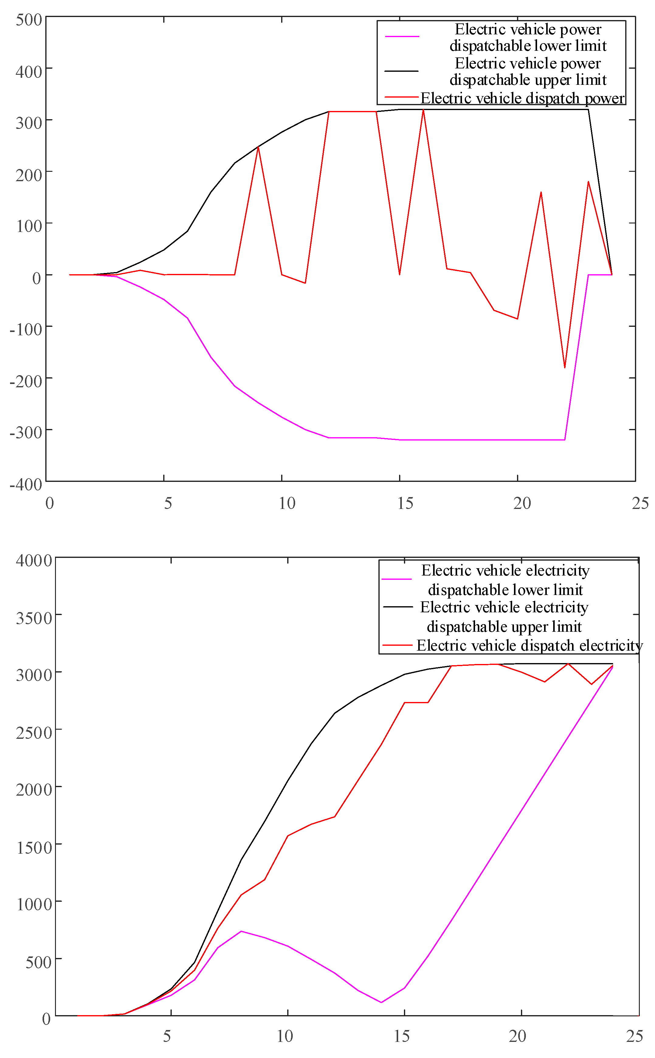
Electric vehicles have the characteristics of small capacity and large scale. Only through the participation of electric vehicle aggregators as a whole in optimized scheduling can they exert flexibility. Cluster electric vehicles have a fast response time and can provide a large amount of two-way flexible supply. Its supply capacity is mainly constrained by the power of charging piles and the travel habits of car owners, which can be expressed as:
where: and are the upward and downward flexibility supply of cluster electric vehicles at time t, respectively; PEV,t and EEV,t are the charging and discharging power and electric energy of cluster electric vehicles at time t, respectively; and are the upper and lower limits of the charging and discharging power of cluster electric vehicles at time t, respectively; and are the upper and lower limits of the electric energy of cluster electric vehicles at time t, respectively.
The feasible domain of charging and discharging power of EVs is not only constrained by the upper and lower limits of its own power, but also affected by electric energy. In this paper, we utilize the extreme scenario method, integrate the parameters of EVs and charging piles, as well as the travel habits of vehicle owners, and establish a general model for single EVs with a feasible domain of half-planar polyhedral sets.
Figure 2.
Modeling principle of EV.
2.3. Flexibility Balance
The flexibility balance of the power system refers to the ability of the total flexibility supply of flexibility resources to meet the flexibility demand of net load. By integrating the flexibility supply capacity of various resources, we can get:
where: and are the upward and downward flexibility supply of the power grid at time t.
The flexibility margin of the power grid is:
where: and are the upward and downward flexibility demands of the power grid at time t, respectively; Δ and Δ are the upward flexibility margin and downward flexibility margin of the power grid, respectively.
When the margin is less than 0, there will be a flexibility deficit, that is:
where: and are the upward and downward flexibility deficits of the grid at time t, respectively.
After calculating the flexibility supply of various resources in the power system, the flexible adjustment factor can be defined as shown in formula (20).
where: and are the upward and downward flexible adjustment factors of various flexibility resources, respectively, indicating the proportion of flexibility resources in meeting the grid flexibility demand at time t, reflecting the contribution of different flexibility resources to ensuring the flexibility balance of the power system.
When , it means that the upward flexibility supply capacity of the flexibility resources can fully track the upward flexibility demand of the power system; when , it means that the downward flexibility supply capacity of the flexibility resources can fully track the downward flexibility demand of the power system. At this time, the power system flexibility has no shortage or redundancy.
It should be noted that the flexibility supply of flexible resources includes ramp capacity and spare capacity, so the capacity spare that flexible resources can provide belongs to flexible capacity.
2.4. Model Transformation
The power balance constraints must be met at each moment:
where: , and are the predicted values of load, wind power and photovoltaic power of the power system at time t, respectively.
2.4.1. Conventional Unit Constraints
Since this paper studies the day-ahead time scale, it is assumed that the unit is in a normally open state and the start and stop of the unit are ignored. The constraints of the thermal power unit include ramp and power constraints, which are expressed as:
where: PG,t is the power generation capacity of the thermal power unit at time t; and are the upper and lower limits of the thermal power unit output.
2.4.2. Pumped Storage Power Station Constraints
Pumped storage hydropower stations are similar to energy storage unit models and can be divided into two states: power generation and pumping. They cannot be operated simultaneously during operation. For conventional pumped storage power stations, the power generation can be continuously changed, while the pumping power cannot be adjusted to a constant value, and the following constraints are met:
where: and are the upper and lower limits of the pumped storage power station’s pumped power; UP.t is an operating state variable, which is 1 for power generation and 0 for pumping; and are the power generation and pumping power of the pumped storage power station; PP.t is the pumped power of the power station at time t, with power generation being a positive value and pumping being a negative value.
At the same time, the reservoir of the pumped storage power station stores water at the beginning and end of each regulation cycle to maintain the balance of the reservoir storage volume and ensure its cyclical participation in power grid regulation. The pumped power of the pumped storage power station and the reservoir energy storage satisfy the following relationship:
where: ηP is the pumping efficiency of the pumped storage power station; T is the total dispatching period; W is the initial energy storage of the reservoir; W and W are the upper and lower limits of the energy storage of the power station reservoir during the regulation process.
2.4.3. Conventional Transferable Load Constraints
When conventional transferable loads perform demand response, the adjustment of the power consumption plan is affected by the power demand, and the power consumption characteristics that are satisfied can be expressed as:
where: DTL is the total power demand of the transferable load during the period of grid dispatch; PTL,t is the power of the transferable load at time t; and are the upper and lower limits of the power.
3. Based on a Data-Driven DRO Model
3.1. Deterministic Model
This paper introduces flexibility deficiency penalty to quantify flexibility and constructs a flexible dispatch model with the lowest total grid operation cost as the objective function. The objective function without considering new energy and load uncertainty is:
where: F1 is the operating cost; F2 is the penalty cost for the lack of flexibility. According to the policy of giving priority to new energy access to the grid, this paper assumes that all wind and photovoltaic power are absorbed and do not participate in the optimization and dispatching of the power grid.
The grid operation costs include the coal consumption costs of thermal power units, the peak regulation costs of pumped storage, the transferable load compensation costs, and the discharge loss compensation costs of cluster electric vehicles.
where: CG,t Cp,t,CTL,t and CEV,t are the coal consumption cost of thermal power units, peak-shaving cost of pumped storage, compensation cost of transferable loads and discharge loss cost of cluster electric vehicles in the power grid at time t, respectively; T is the dispatch period; a, b and c are the cost coefficients of thermal power units; and are the power generation and pumping power of the pumped storage power station at time t, respectively; KP is the unit peak-shaving cost of pumped storage; KTL is the unit compensation cost of transferable loads participating in demand response; KEV is the unit discharge compensation cost of cluster electric vehicles; is the discharge power of cluster electric vehicles at time t; is the expected electricity demand of residents at time t. By introducing auxiliary variables PTL1,t and PTL2,t and adding constraints as shown in Equations (33) and (34), the transferable load compensation cost is equivalent to a linear form as shown in Equation (35).
The coal consumption cost function of the thermal power unit is piecewise linearized to improve the model calculation speed, and the coal consumption cost of the thermal power unit becomes:
where: Ks is the slope of each segment after the original quadratic function is piecewise linearized; S is the number of segments; CG,0 is the cost of coal consumption generated when the thermal power unit operates at the minimum output ; PG,t,s is the segmented output of the unit, satisfying formula (38).
When the power system flexibility margin is insufficient, it will be penalized. The flexibility deficiency penalty cost is expressed as the sum of the upward flexibility deficiency penalty cost and the downward flexibility deficiency penalty cost, as shown in formula (39).
where: Cdefc,t is the flexibility deficit penalty cost of the power grid at time t; Kdefc is the flexibility deficit penalty factor.
3.2. Two-Stage DRO Model
In order to find the optimal flexible scheduling solution under the probability distribution of the worst scenario, this section establishes a data-driven DRO model based on the historical sample data of load and new energy. The DRO involved in this article is a two-stage min-max-min three-layer optimization problem. The first stage min problem uses the output of each flexibility unit on the power supply side as the decision variable to achieve the optimal economic operation goal. The second stage max-min problem finds the probability distribution of the worst scenario that maximizes the minimum value of the demand-side resource call cost and the grid flexibility shortage penalty cost. The expression is as follows:
where: x is the variable in the first stage; y is the variable in the second stage; K is the number of discrete scenarios; pk is the probability of the occurrence of the kth scenario; r(x, ξk) is the objective function value of the inner minimum problem; ξk is the kth scenario; yk is the variable in the second stage under the kth scenario; f1 is the output cost of each unit on the power supply side; f2 is the resource call cost on the demand side and the penalty cost of the grid flexibility shortage; Ω is the comprehensive norm fuzzy set; U (x, ξk) is the feasible domain of the optimization variable yk when a set (x, ξk) is given; h (x) ≤ 0 is a constraint related only to the first stage, without considering the uncertainty of the probability of new energy and load scenarios, and is a deterministic constraint; g (x, pk, yk) ≤ 0 is the constraint in the second stage.
Since the uncertain probability set of load and new energy is difficult to obtain, this paper adopts a data-driven method to obtain K discrete typical scenarios (ξ1, ξ2, …, ξK) in M samples of historical data through a probability-based reduction method to characterize the possible values of uncertain information, and uses this probability distribution as the initial probability distribution. Considering that the discrete values of each reduction scenario are still uncertain, in order to ensure that the value of the scenario probability fluctuates within a reasonable range, a comprehensive norm constraint centered on the above initial probability distribution is constructed to restrict the probability distribution of the uncertain scenario, making it closer to the real scenario. The comprehensive norm constraint includes 1-norm and ∞-norm, as shown in Equation (45) and Equation (46), respectively. The constructed comprehensive norm fuzzy set is shown in Equation (47).
where: ‖⋅‖1 is the 1-norm; ‖⋅‖∞ is the ∞-norm; is the probability distribution value of the initial scenario; θ∞ and θ1 are the deviation values allowed by the probability distribution under the ∞-norm and 1-norm constraints, respectively. It can be seen from the literature [27] that the probability distribution {pk} satisfies the confidence constraints of equations (48) and (49).
Let the right sides of equations (48) and (49) be the uncertainty probability confidence levels α1 and α∞, respectively. Under a confidence level of 95%, equations (48) and (49) guarantee that there is at least a 95% probability that a fuzzy distribution exists in a given set [27]. θ∞ and θ1 can be calculated by equation (50).
The deviation values of θ∞ and θ1 indicate the maximum value by which the DRO scenario probability can deviate from the initial scenario probability. The larger the value, the more conservative the robust model is, and vice versa.
4. Two-Stage Model Solving Algorithm
Two-stage distributed robust optimization is usually based on the idea of zero-sum game, and uses the column and constraint generation (C&CG) algorithm or the cutting plane (Benders) algorithm to solve the original problem, decoupling it into a main problem and sub-problems for iteration. Compared with the Benders algorithm, the C&CG algorithm continuously introduces auxiliary variables and constraints related to the sub-problems in the process of solving the main problem, which speeds up the convergence speed.
Decomposing the two-stage model (i.e., (40) to (42)), the master problem (MP) is:
where: l is the number of iterations; θ is the relaxation amount of the subproblem; y is the auxiliary variable related to the subproblem introduced at the l-th iteration; p is the worst scenario probability of wind and photovoltaic load obtained by solving the subproblem at the l-th iteration, which is a known quantity.
The purpose of the sub-problem is to find the worst scenario probability distribution that maximizes the minimum value of the demand-side resource call cost and the grid flexibility deficiency penalty cost. When the variables in the first stage are given, the sub-problem can be expressed as:
where: x* is the solution to the main problem, and is a known quantity here.
Although the form of the subproblem is an NP-hard max-min double-layer optimization problem, it is not difficult to find that the inner min problems in each scenario are independent of each other, and the inner min problems can be solved simultaneously using parallel computing methods. Therefore, the subproblem can be rewritten as two single-layer optimization problems that are solved in sequence, as shown in formula (53).
Equation (53) is a mixed integer programming, which can be quickly solved using the Gurobi solver. The result {pk} obtained is the probability distribution of the worst scenario, which is passed to the main problem for iterative calculation.
The specific solution process is as follows:
- Start
-
Collect historical wind-photovoltaic-load dataGather historical sample data for wind, photovoltaic, and load.
-
Construct copula temporal and spatial correlation output setUse the collected data to build the Copula temporal and spatial correlation output set.
-
Initialize iteration parametersSet the lower bound LB of the second-stage cost to -∞ and the upper bound UB to +∞.Set the iteration counter l to 1.
-
Main problem optimizationSolve the main optimization problem considering the worst-case scenario probability distribution.Update the upper bound UB and lower bound LB based on the solution.
-
Check iteration termination conditionsIf the termination conditions (e.g., convergence of UB and LB, maximum number of iterations reached) are met, proceed to the next step.Otherwise, go back to the Main Problem Optimization step.
-
Update worst-case scenario probability distributionSolve the subproblem to update the probability distribution of the worst-case scenario.
-
Obtain optimal solutionAfter the iteration terminates, obtain the optimal solution for the wind-photovoltaic-load management problem.
- End
5. Results and Discussion
The algorithms were solved through MATLAB 2018b platform and Gurobi solver. The time scale for flexible dispatch before the day in this paper is taken as 1 h. The wind and light load data samples are randomly generated using normal distribution on the basis of the predicted values, and the number of samples is taken as 500, and the probability distribution of the initial scenario is obtained by probabilistic distance-based scenario cutting technique, and the number of scenarios after cutting is 5, and the typical scenario curves are shown in the literature [19]. The maximum fluctuation coefficients of εL, εW and εPV for the load, wind power and PV in the day before yesterday are 0.05, 0.10 and 0.08, respectively, and the parameters of each unit of the calculation example are shown in Table 1.
5.1. Power System Flexibility Balancing Results
In this section, four flexibility regulation scenarios are set up to analyze the impact of the participation of load-side resources in the flexibility supply and the inclusion of flexibility balancing constraints on the flexibility margin of the power system during the day-ahead scheduling phase.
Scheme 1: Load-side resources do not participate in demand response (transferable loads are considered as fixed loads and Evs are charged in a disorderly manner), and flexibility balancing constraints are not considered.
Scheme 2: Load-side resources participate in demand response (orderly charging and discharging of Evs) without considering flexibility balancing constraints.
Scheme 3: Load-side resources participate in demand response, taking into account flexibility balancing constraints.
Scheme 4: Load-side resources do not participate in demand response, considering flexibility balancing constraints.
Since Scheme 1 and 2 do not consider flexibility constraints, the flexibility demand and flexibility supply of the power system are then calculated at the end of the optimal scheduling. The Scheme 3 grid flexibility margins are shown in Figure 3. The net load curve of Scenario 3 is flatter in the 16:00-22:00 hours, i.e., the uphill and downhill sections of the evening peak, reducing the flexibility demand of the grid, so that there are sufficient upward and downward flexibility margins in all hours except 19:00.
Table 2 shows the operating costs and flexibility balances for each Scheme. Scheme 1 does not consider demand response and does not optimize the flexibility supply and demand, so there is a large flexibility deficit in the grid. Schemes 2 and 3 take into account the transferability of loads, and although they require some call subsidy costs, the total operating cost and flexibility deficit are lower than in Scenario 1. Scenario 3 takes into account the flexibility balancing constraints in comparison to Scheme 2, and requires more demand-side resources to be called upon, so the total operating cost is slightly higher, but the flexibility deficit is significantly reduced, which ensures that the system is flexible with a small reduction in the economic performance. The flexibility of Scheme 4 is only supplied by the power side, although the flexibility balancing constraint is considered on the basis of power balancing, it only works on the power side resources, and the adjustment range Is not large, so there Is still a large amount of flexibility shortfall, and the operating cost Is close to that of Scheme 1.
5.2. Analysis of Flexibility Adjustment Capacity for Flexibility Resources
In this paper, a flexibility adjustment factor is introduced in the participation of various types of flexibility resources in maintaining the flexibility balance of the grid to reflect the degree of contribution of different flexibility resources to ensure the flexibility balance of the grid. The larger the flexibility adjustment factor of a flexibility resource at time t is, the stronger the flexibility adjustment capability of the resource is. When the sum of the flexibility adjustment factors of all types of resources is less than 1, it means that the power system has a flexibility shortage at time t. Conversely, when the sum of the flexibility adjustment factors is greater than 1, it indicates that flexibility is left in reserve.
Figure 4 shows the contribution of different flexibility resources to take up the flexibility needs of the grid in scheme 3, where the red dashed line indicates that the flexibility resources fully track the flexibility needs of the grid.
In Figure 4(a), the sum of the flexibility regulation factors at the 19:00 hour is below the red line, which means that there is a shortage of flexibility at that hour, which is consistent with the analysis results in Section 4.1. From Fig. 4(a) and (b), it can be seen that the flexibility regulation ability of each type of flexibility resource is different in each time period. The flexibility of thermal units is limited by capacity and ramp-up, and can only withstand baseload, so the downward flexibility supply capability is better than the upward flexibility supply capability as a whole. During 10:00-12:00 load trough hours, thermal units operate at lower output levels and can only provide a small amount of downward flexibility supply. During the 13:00-20:00 net load rise period, thermal power units are only supplied with ramping capacity for upward flexibility. Pumped storage power plants pump water and generate electricity at sharp net load fluctuations, with strong flexibility, effectively compensating for the lack of climbing capacity of thermal power units in a short period.
Cluster EVs should take into account the travel needs of their owners when participating in vehicle-network interactions: choosing to charge at maximum power during the 12:00-16:00 net load trough hour provides a lot of upward flexibility; discharging during the 19:00-21:00 evening peak hour provides only a small amount of downward flexibility. It should be noted that EVs are also discharged near the 10:00 hour due to the risk of insufficient downward flexibility of the grid at that hour, and the charging and discharging behavior of cluster EVs is adequately managed due to the flexibility balance constraints considered in this paper. The transferable loads are limited by electricity demand and capacity, and can provide less flexibility by transferring peak loads, whose downward flexibility supply is slightly larger than the upward flexibility supply.
5.3. Conservativeness Analysis of Data-Driven DRO Models
Given uncertainty probability confidence levels α1 and α∞ of 0.5 and 0.99, respectively, the effect of different historical sample sizes M and the number of typical scenarios cut K on the degree of conservatism of the DRO model is investigated.
As can be seen in Table 3, as the number of historical samples increases, the cost of operation and flexibility deficit of each unit of the grid decreases. This is due to the fact that the increase in the number of historical samples makes the deviation values θ∞ and θ1 allowed by the probability distribution decrease accordingly, and the conservatism of the DRO model is alleviated.
Table 4 shows the effect of the number of typical scenarios on the model conservatism after sample data reduction, and it is easy to find that the conservatism degree increases with the number of scenarios. This is because as the number of typical scenarios becomes larger, the resolution of the cut scenarios becomes larger, and the probability that the extreme data in the original large amount of sample data become a class of typical scenarios alone becomes higher. Typical scenarios are portrayed more and more finely, closer to the actual fluctuation range of wind and photovoltaic loads, and the robustness of the model is improved.
The conservatism of the DRO model in this paper is reflected in the fact that the probability of occurrence of severe scenarios of net load fluctuations becomes higher. Both the static equilibrium of power supply and demand are reflected and the fluctuating process of power supply and demand, i.e., the flexibility equilibrium process, is highlighted. The small change in the cost of thermal units when the model conservatism increases is related to their tracking of base load. The increased total operating costs mainly come from the demand response compensation costs of load-side resources, which results in a smaller increase in the flexibility deficit of the power system, proving the validity of the proposed model.
5.4. Comparative Analysis with Other Uncertainty Optimization Methods
The data-driven DRO model (the model in this paper), which takes into account the correlation of wind and scenery output, is compared with the data-driven DRO model without considering the correlation of wind and scenery output, the traditional two-stage RO model, and the SO model. The uncertainty probability confidence level α1 and α∞ of the data-driven DRO model are 0.5 and 0.99, respectively, and the number of samples M and the number of cut scenarios K are taken as 500 and 5, respectively. The results of the four models are shown in Table 5.
As can be seen from Table 5, the four models have a small difference in the operating cost of each unit on the power side and a large difference in the demand response cost. the RO model is the most robust considering the worst peak climbing scenario with uncertain information, so it has the largest cost and flexibility shortfall in all aspects. The data-driven DRO model synthesizes the advantages of the RO model and the SO model, and uses comprehensive paradigm constraints to construct a probability distribution fuzzy set, which has better economy and flexibility, and the economy and robustness in the day-ahead scheduling phase are taken as a compromise. When the temporal and spatial correlation of wind and photovoltaic output is described by Copula theory, the calculated grid flexibility demand is smaller due to the consideration of wind and photovoltaic complementarity, and the model proposed in this paper is less conservative compared to the data-driven DRO model that does not consider the wind and photovoltaic correlation. At the same time, since the data-driven DRO model does not require pairwise processing in the subproblem processing compared to the RO model, the parallel computation method it adopts reduces the computation time significantly.
6. Conclusions
This paper proposes a data-driven distributed robust optimization (DRO) model that considers flexibility balance. By comparing simulation examples, the following conclusions are obtained:
1) By combining the interval method with the scenario-based approach within the DRO framework, we quantify flexibility demand while fully accounting for net load fluctuations across various scenarios. Under the constraint of flexibility supply and demand balance, load-side resources such as electric vehicles and conventional transferable loads participate in demand response, providing significant ramping capacity. This effectively reduces net load fluctuations. By considering the flexibility supply capabilities of demand-side resources, the overall flexibility of the power grid is improved, particularly during morning and evening peak hours with high ramping demands. Flexibility margins are notably enhanced, ensuring power system flexibility while only marginally compromising economic performance.
2) The data-driven DRO model thoroughly considers the uncertainty of renewable energy and load fluctuations based on historical data samples. When the degree of conservatism increases, the power grid needs to offer more economic incentives to load-side resources to encourage their participation in demand response. These incentives motivate load-side resources to provide additional flexibility, addressing the challenges posed by adverse net load ramping scenarios. By offering economic compensation, the grid ensures that load-side resources are willing to contribute to flexibility provision, thereby enhancing the overall resilience of the power system against uncertainty.
3) The DRO model not only achieves a compromise between economy and robustness in the day-ahead scheduling stage but also demonstrates superior resilience against uncertainty fluctuations in real-time operations. By leveraging historical data and considering a distribution of possible outcomes, the DRO model is able to better manage uncertainty and risk. Compared to Stochastic Optimization (SO) models, the DRO model exhibits better overall economic performance. It provides a more robust solution that can withstand uncertainty while maintaining economic efficiency, making it a valuable tool for power system flexibility management in the face of increasing renewable energy penetration and load variability.
Author Contributions
Conceptualization, Jinniu Miao; Methodology, Liqian Zhao; Supervision, Lei Sun and Wei Zhao; Writing – original draft, Jiaji Liang; Writing – review & editing, Jingyang Wu and Peng Du; Validation, Benrui Zhu.
Funding
This research was funded by Research Project of National Petroleum and Natural Gas Pipeline Network Group Co., Ltd "Research on Comprehensive Application Technology of Photovoltaic Power Generation in Oil and Gas Storage and Transportation Engineering"., grant number DTXNY202202. We also greatly appreciate the helpful suggestions and comments of editors and reviewers.
Conflicts of Interest
The authors declare no conflicts of interest.
References
- LU Xi, MCELROY Michael B, PENG Wei, et al. Challenges faced by China compared with the US in developing wind power[J]. Nature Energy, 2016, 1(6): 16061. [CrossRef]
- LU Zongxiang, LI Hao, QIAO Ying. Morphological evolution of power systems with high share of renewable energy generations from the perspective of flexibility balance[J]. Journal of Global Energy Interconnection, 2021, 4(01): 12-18. [CrossRef]
- LU Zongxiang, LIN Yisha, QIAO Ying, et al. Flexibility supply-demand balance in power system with ultra-high proportion of renewable energy[J]. Automation of Electric Power Systems, 2022, 46(16): 3-16. [CrossRef]
- HU Junjie, LIU Xuetao, WANG Cheng. Value evaluation of energy hub flexibility considering network constraints[J]. Proceedings of the CSEE, 2022, 42(5): 1799-1813. [CrossRef]
- JI Xingquan, LIU Jian, ZHANG Yumin, et al. Optimal dispatching of integrated energy system considering operation flexibility constraints[J]. Automation of Electric Power Systems, 2022, 46(16): 84-94. [CrossRef]
- ZHOU Guangdong, ZHOU Ming, SUN Liying, et al. Research on operational flexibility evaluation approach of power system with variable sources[J]. Power System Technology, 2019, 43(6): 2139-2146. [CrossRef]
- ZHAN Xunsong, GUAN Lin, ZHUO Yingjun, et al. Multi-scale flexibility evaluation of large-scale hybrid wind and photovoltaic grid-connected power system based on multi-scale morphology[J]. Power System Technology, 2019, 43(11): 3890-3901. [CrossRef]
- LU Zongxiang, LI Haibo, QIAO Ying. Flexibility evaluation and supply/demand balance principle of power system with high-penetration renewable electricity[J]. Proceedings of the CSEE, 2017,37(1): 9-20. [CrossRef]
- SUN Donglei, SUN Keqi, YANG Jinye, et al. Power system optimal dispatch considering the requirements of flexibility[J]. Journal of Shandong University (Engineering Science), 2022, 52(1): 120-127. [CrossRef]
- ZHANG Gaohang, LI Fengting. Day-ahead optimal scheduling of power system considering comprehensive flexibility of sourceload-storage[J]. Electric Power Automation Equipment, 2020, 40(12):159-167. [CrossRef]
- TANG Xiangying, HU Yan, GENG Qi, et al. Multi-time-scale optimal scheduling of integrated energy system considering multi-energy flexibility[J]. Automation of Electric Power Systems, 2021, 45(4): 81-90. [CrossRef]
- HUANG Pengxiang, ZHOU Yunhai, XU Fei, et al. Source-load-storage coordinated rolling dispatch for wind power integrated power system based on flexibility margin[J]. Electric Power, 2020, 53(11): 78-88. [CrossRef]
- ZHAO Fulin, ZHANG Tong, MA Guang, et al. Study on flexible operation region of power system considering source and load fluctuation[J]. Journal of Zhejiang University (Engineering Science), 2021, 55(5): 935-947. [CrossRef]
- KHATAMI Roohallah, PARVANIA Masood, NARAYAN Akil. Flexibility reserve in power systems definition and stochastic multi-fidelity optimization[J]. IEEE Transactions on Smart Grid, 2020, 11(1): 644-654. [CrossRef]
- XU Hao, LI Huaqiang. Planning and operation stochastic optimization model of power systems considering the flexibility reformation[J]. Power System Technology, 2020, 44(12): 4626-4638. [CrossRef]
- WANG Tao, HU Li, LIU Zihan, et al. Distributionally robust real-time dispatch model considering flexibility requirement and correlations of wind powers[J]. Journal of Global Energy Interconnection, 2021, 4(6), 585-594. [CrossRef]
- SHUI Yue, LIU Junyong, GAO Hongjun, et al. A distributionally robust coordinated dispatch model for integrated electricity and heating systems considering uncertainty of wind power[J]. Proceedings of the CSEE, 2018, 38(24): 7235- 7247. [CrossRef]
- HE Shuaijia, RUAN Hebin, GAO Hongjun, et al. Overview on theory analysis and application of distributionally robust optimization method in power system[J]. Automation of Electric Power Systems, 2020, 44(14): 179-191. [CrossRef]
- RUAN Hebin, GAO Hongjun, LIU Junyong, et al. A distributionally robust reactive power optimization model for active distribution network considering reactive power support of DG and switch reconfiguration[J]. Proceedings of the CSEE, 2019, 39(3): 685-695. [CrossRef]
- SHI Zhichao, LIANG Hao, HUANG Shengjun, et al. Distributionally robust chance-constrained energy management for islanded microgrids [C]// IEEE Power & Energy Society General Meeting, -8, 2019, Atlanta, USA: 1-7. 4 August. [CrossRef]
- WU Jiechen, AI Xin, HU Junjie. Methods for characterizing flexibilities from demand-side resources and their applications in the day-ahead optimal scheduling[J]. Transactions of China Electrotechnical Society, 2020, 35(9): 1973-1984. [CrossRef]
- WANG Pingping, XU Jianzhong, YAN Qingyou, et al. A two-level scheduling optimization model for building microgrids considering demand response and uncertainties of flexible load resources[J]. Electric Power Construction, 2022, 43(6): 128-140. [CrossRef]
- CUI Mingjian, ZHANG Jie, WU Hongyu, et al. Wind-friendly flexible ramping product design in multi-timescale power system operations[J]. IEEE Transactions on Sustainable Energy, 2017, 8(3): 1064-1075. [CrossRef]
- HANG Bo, SHEN Jianjian, CHENG Chuntian, et al. Peak-shaving method of hydro-wind power complementary system based on C-vine Copula theory[J]. Proceedings of the CSEE, 2022, 42(15): 5523-5535. [CrossRef]
- Li Jingxuan, Zhou Ming, Zhu Lingzhi, et al. Flexibility Requirement Quantifying and Optimal Dispatching for Renewable Integrated Power Systems [J]. Power System Technology, 2021, 45(07): 2647-2656. [CrossRef]
- Yang Nan, Huang Yu, Ye Di, et al. Modeling of Output Correlation of Multiple Wind Farms Based on Adaptive Multivariable Nonparametric Kernel Density Estimation[J]. Proceedings of the CSEE, 2018, 38(13): 3805-3812+4021. [CrossRef]
- ZHAO Chaoyue, GUAN Yongpei. Data-driven stochastic unit commitment for integrating wind generation[J]. IEEE Transactions on Power Systems, 2016, 31(4): 2587-2596. [CrossRef]
Figure 3.
Scheme 3 grid flexibility margin.
Figure 4.
Flexibility adjustment ability of different flexible resources.
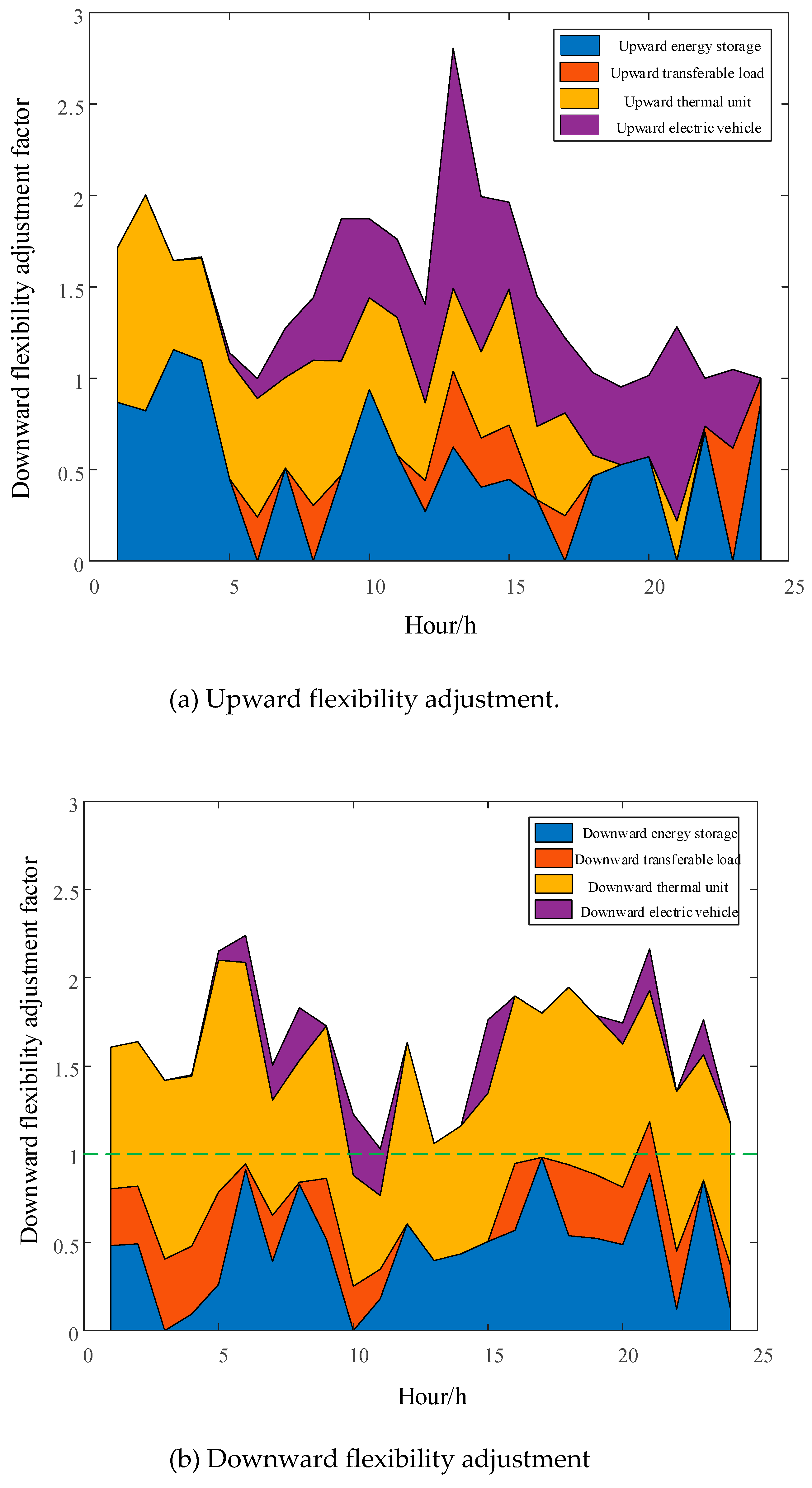

Table 1.
Algorithm-related parameters.
| Unit equipment | Variable | Numerical value |
| Electric vehicle | N[9,1]h | |
| N[20,2]h | ||
| 6kW | ||
| -6kW | ||
| N[25.6,6.4]kW·h | ||
| 6.4kW·h | ||
| 64kW·h | ||
| 64kW·h | ||
| 0.64 | ||
| Thermal unit | 300kW | |
| 1500kW | ||
| 280kW/h | ||
| Pumped storage | 1000kW·h | |
| 300kW·h | ||
| 0.38 | ||
| 500kW | ||
| 500kW·h | ||
| 0.85 | ||
| Conventional transferable load | 0.32 | |
| 2840kW·h | ||
| 50kW·h | ||
| 250kW·h |
Table 2.
Comparison of operation cost and flexibility balance of each scheme.
| Scheme | Operation cost/RMB | Total operation cost/RMB | Flexibility gap/(kW·h) | |||
| Thermal unit | Transferable load | Electric vehicle | Pumped storage | |||
| 1 | 22116.6 | 0 | 0 | 1232.1 | 23348.7 | 4445 |
| 2 | 20821.2 | 834.1 | 190.6 | 1077.2 | 22923.1 | 1311 |
| 3 | 20903.9 | 910.5 | 218.3 | 1080.1 | 23112.8 | 48 |
| 4 | 22221.1 | 0 | 0 | 1301.2 | 23522.3 | 3982 |
Table 3.
Analysis of number of historical samples.
| M | Operation cost/RMB | Total operation cost/RMB | Flexibility gap/(kW·h) | |||
| Thermal unit | Transferable load | Electric vehicle | Pumped storage | |||
| 500 | 20903.9 | 910.5 | 218.3 | 1080 | 23112.8 | 48.0 |
| 1000 | 20653.2 | 899.2 | 209.2 | 1002 | 22763.6 | 46.2 |
| 2000 | 20611.5 | 873.4 | 201.3 | 1002 | 22688.3 | 41.9 |
| 5000 | 20542.8 | 868.4 | 201.3 | 1002 | 22614.5 | 41.9 |
Table 4.
Analysis of number of typical scenarios.
| K | Operation cost/RMB | Total operation cost/RMB | Flexibility gap/(kW·h) | |||
| Thermal unit | Transferable load | Electric vehicle | Pumped storage | |||
| 500 | 20903.9 | 910.5 | 218.3 | 1080 | 23112.7 | 48.0 |
| 1000 | 20921.1 | 914.2 | 221.2 | 1082 | 23138.5 | 48.0 |
| 2000 | 20958.3 | 916.1 | 222.5 | 1086 | 23182.9 | 52.8 |
| 5000 | 20961.9 | 922.3 | 228.1 | 1090 | 23202.3 | 74.0 |
Table 5.
Comparison of results of different models.
| K | Operation cost/RMB | Total operation cost/RMB | Flexibility gap/(kW·h) | |||
| Thermal unit | Transferable load | Electric vehicle | Pumped storage | |||
| 500 | 20903.9 | 910.5 | 218.3 | 1080 | 23112.7 | 48.0 |
| 1000 | 20921.1 | 914.2 | 221.2 | 1082 | 23138.5 | 48.0 |
| 2000 | 20958.3 | 916.1 | 222.5 | 1086 | 23182.9 | 52.8 |
| 5000 | 20961.9 | 922.3 | 228.1 | 1090 | 23202.3 | 74.0 |
Disclaimer/Publisher’s Note: The statements, opinions and data contained in all publications are solely those of the individual author(s) and contributor(s) and not of MDPI and/or the editor(s). MDPI and/or the editor(s) disclaim responsibility for any injury to people or property resulting from any ideas, methods, instructions or products referred to in the content. |
© 2025 by the authors. Licensee MDPI, Basel, Switzerland. This article is an open access article distributed under the terms and conditions of the Creative Commons Attribution (CC BY) license (http://creativecommons.org/licenses/by/4.0/).
Copyright: This open access article is published under a Creative Commons CC BY 4.0 license, which permit the free download, distribution, and reuse, provided that the author and preprint are cited in any reuse.


