
Submitted:
18 January 2025
Posted:
20 January 2025
You are already at the latest version
Abstract
Data for growth (birth, weaning and yearling weights) and carcass (longissimus muscle area, percent intramuscular fat and depth of rib fat) traits and 50K SNP marker data to calculate the genomic relationship matrix were collected from 738 Brangus heifers. Univariate and multivariate artificial neural networks with 1 to 10 neurons models including the inputs from genomic relationship matrix were created and applied with the learning algorithms of Bayesian Regularization, Levenberg–Marquardt and Scaled Conjugate Gradient and transfer function combinations of tangent sigmoid-linear and linear-linear in the hidden-output layers for the analysis of growth and carcass data. Pearson’s correlation coefficients were used to evaluate the predictive performances of univariate and multivariate ANN models. The overall predictive ability of artificial neural network models was low in the univariate and multivariate analysis. However, the predictive performances of models in the univariate analysis were significantly higher than those from models in the multivariate analysis. In the univariate analysis, models with Bayesian Regularization and the tangent sigmoid-linear or linear-linear transfer function combination yielded higher predictive performances than those in learning algorithms. In addition, predictive performances of models with tangent sigmoid-linear transfer functions were better than those with linear-linear transfer functions in the univariate analysis.
Keywords:
genomic prediction
; genomic relationship
; artificial neural network
; learning algorithm
; transfer function
1. Introduction
There is a growing interest in improving the economically important traits in beef cattle breeding programs to increase the profitability of beef cattle production systems. Among the several economically important traits, growth-related traits including birth weight (BW), weaning weight (WW), yearling weight (YW) are traditionally considered as selection criteria in beef cattle breeding. Carcass traits including longissimus muscle area (LMA), percent intramuscular fat (IMF), depth of rib fat (FAT) have also gained importance in the selection programs of beef cattle breeding in order to fulfill the market quality standards and the consumer perceptions of meat [1,2,3]. Genomic selection has been applicable for economically important traits since the availability of high-density single nucleotide polymorphism (SNP) markers [1,2,3,4] and the statistical methods for genomic prediction [1,5,6]. Many statistical methods (such as GBLUP, BayesA, BayesB, BayesC, and Bayesian Lasso) for genomic prediction work based on capturing the association between SNP marker genotypes and phenotypes of a trait and then by fitting the association, learn how SNP marker genotypes map to the quantity to be predicted.
In last decade, artificial neural networks (ANN) were considered as a different learning method for genomic prediction. The development and use of ANN for artificial intelligence was inspired from the operations of nerve cells (known neurons) in the human brain. The ANN is a statistical modeling of the human brain functions and represents a new generation of information processing systems [7]. The learning ability of ANN without using any prior assumption and sophisticated statistical models for linear and nonlinear relationships in the information processing systems is a very attractive feature. ANN methods are nonparametric models providing tremendous flexibility to adapt to complicated associations between data and output. A particular strength is the ability to adapt to hidden patterns of unknown structure that therefore could not be incorporated into a parametric model at the beginning [8]. Therefore, ANN statistical models have been used to predict genomic values of individuals for complex traits for last decade because complex quantitative traits such as growth and production traits in animal and plant breeding are controlled by a network of numerous genes [9]. This study aimed to compare the predictive performances of univariate and multivariate ANN-1-10-neuron models with the learning algorithms (Levenberg–Marquardt (LM), Bayesian Regularization (BR) and Scaled Conjugate Gradient (SCG)) and transfer functions (tangent sigmoid and linear) using the input from G genomic relationship matrix in analyses of growth and carcass traits.
2. Materials and Methods
2.1. Phenotypes, SNP Markers and Genomic Relationship Matrix
Data for growth (birth weight (BW), weaning weight (WW) and yearling weight (YW)) and carcass (longissimus muscle area (LMA), percent intramuscular fat (IMF), and depth of rib fat (FAT)) traits were obtained from 738 Brangus heifers which raised in Camp Cooley Ranch in east central Texas, the Chihuahuan Desert Rangeland Research Center and Campus Farm of New Mexico State University in the spring or fall calving season of 2005 through 2007 birth years [10,11,12].
SNP marker genotypes (AA, AB, BB) of 738 Brangus heifers were obtained by using BovineSNP50 Infinium BeadChips (Illumina, San Diego, CA) for 53,692 SNP markers [2]. Three filters were applied for the quality control of SNP markers using the snpReady package in R-program [13]: Heifers were retained where a) the genotype call rate was greater than 95% and b) the number of missing observations was less than 50% and c) SNP markers with minor allele frequency (MAF) greater than 10% were retained. Then, the imputation of missing SNP marker genotypes resulted in 738 animals with 35,351 SNP markers.
Genomic relationship matrix () [14,15] was calculated by using 35,351 SNP markers as
where is the matrix of the coded (0 for AA, 1 for AB, 2 for BB) SNP marker genotypes for the animals; is the matrix for allele frequencies of the SNP markers multiplied by 2, is the allele frequency of ith SNP marker, and the sum is over all loci.
2.2. Artificial Neural Networks
Artificial neural network (ANN) is a type of non-linear model frequently used to predict genomic breeding values for genomic selection in the last decade. ANN models are computer algorithms and their working principles are inspired by the function of the human brain and nervous system. The neurons of human brain and their connections with each other establish the relationship among neurons as data processing units connected via adjustable weights () in ANN. ANN consists of an input layer, hidden layer(s), and an output layer. The interconnected neurons are arranged based on their functions in layers.
The Multi-Layer Perceptron Artificial Neural Network (MLPANN) includes many interconnected neurons which are grouped into an input layer, an intermediate or hidden layer and an output layer. The graphical representation of the MLPANN used for this study is given in Figure 1. As seen in Figure 1, genomic relationships () between animals are independent variables and represent the input neurons in the input layer of the MLPANN model. Also, the growth (BW, WW and YW) and carcass (LMA, IMF and FAT) traits are dependent variables and represent the output neurons in the output layer of the MLPANN model.
Training process in the MLPANN focuses on increasing the estimation accuracy between predicted (output) values () and the observed (actual) phenotypic values () using the different number of neurons, learning algorithms and transfer functions in the hidden layer and producing the univariate or multivariate outputs in the output layer.
2.2.1. Number of Neurons in Hidden Layer
The number of neurons () in hidden layer has a significant effect on the performance of MLPANN model. The use of too few (one or two) neurons could not be enough to establish the unknown relationship between inputs and outputs in MLPANN model; however, the use of too many neurons in the training process could cause the increase of complexity and execution time of MLPANN model. From literature, it was found that a single hidden layer was sufficient for an MLPANN model to approximate any complex nonlinear function [16,17] neurons between 1 and 10 () was used in the MLPANN model (Figure 1).
2.2.2. Learning Algorithm in Hidden Layer
The learning in ANN for genomic prediction is a training process which occurs by comparing the ANN predicted (output) value () with the observed (actual) phenotypic value () and calculating the prediction error () in the training dataset. The back-propagation of prediction error and the adjustment of the connection weights are iteratively carried out by the learning algorithm [18] which attempts to reduce the global error by adjusting the weights and biases in the ANN procedure. Although many learning algorithms are indicated in the literature for the ANN procedure [19,20,21], it is difficult to determine the efficient one for genomic selection. Therefore, Bayesian Regularization (BR), Levenberg–Marquardt (LM) and Scaled Conjugate Gradient (SCG) backpropagation learning algorithms in this study were used to determine the faster learning and the better estimating ANN algorithm in the analysis of the growth (BW, WW and YW) and carcass traits (LMA, IMF and FAT).
2.2.3. Transfer Functions in Hidden Layer
Transfer (activation) functions are used to calculate the outputs in the hidden and output layers during the training process in the MLPANN model. In this study, tangent sigmoid and linear transfer functions in the hidden layer were applied to calculate the outputs based on the association between inputs and outputs from the hidden layers in the MLPANN model (Figure 1). The tangent sigmoid and linear transfer functions are given in Figure 2:
- Linear transfer function produces an output in the range of to [24,25]. The association between inputs and outputs in the MLPANN models could not be non-linear and is determined by the purelin transfer function which can be an acceptable representation of the input/output behavior in the MLPANN models.
As presented in Figure 2, the input layer in the MLPANN model distributes the genomic relationships values () as an input signal to the neurons in the hidden layer. In the hidden layer, genomic relationships values are combined with a vector of weights , plus a bias () at the hidden neuron () in order to develop the score for animal . Then, the resultant score is transformed using linear or tangent sigmoid activation functions to produce the output of hidden neuron for animal for the growth (BW, WW and YW) and carcass traits (LMA, IMF and FAT).
2.2.4. Univariate or Multivariate Outputs in Output Layer
The MLPANN model is applied for the univariate (single trait) analysis or multivariate (multiple traits) analyses and the univariate or multivariate outputs of neurons in the output layer were calculated by using a transfer function (Figure 1 and Figure 2). The predictive performance of the MLPANN model could be affected by the univariate or multivariate structure of output layer; therefore, in this study,
- the univariate output of neurons in the output layer for the growth (BW, WW and YW) and carcass (LMA, IMF and FAT) traits:where and ,
2.3. Cross-Validation and Predictive Performance of Artificial Neural Networks
Habier et al. [14] studied the effect of genomic relationships between animals in the training and validation data sets and showed that the accuracy of GEBV of animals in validation data set increases when the genomic relationship between animals in validation data set and animals in training data set increases. Saatchi et al. [26] also indicated that minimizing the genomic relationships between animals in training and animals in validation data sets by using k-means clustering approach resulted in less effected accuracies of GEBV of animals in validation data set by their genomic relationships. Therefore, in this study 10-fold cross-validation data sets were created from the genotyped animals by using k-means clustering approach based on the pedigree-base additive relationships [27]. GeneticsPed [28] and factoextra [29] packages in R-program were used to construct the pedigree-base numerator relationship () matrix and 10-fold cross-validation data sets based on k-means clustering approach.
The training and validation processes in the cross-validation approach were carried out by taking nine cross-validation data sets from 10-fold cross-validation data sets to train the ANN and remaining one cross-validation data set to predict phenotypic values of animals from the omitted validation set. The predictive performance of ANN for growth (BW, WW and YW) and carcass (LMA, IMF and FAT) traits was evaluated by pooling the estimates of Pearson’s correlation coefficient () between the observed () and predicted phenotypic () values from 10-fold cross-validation data sets.
where is the covariance between the observed () and predicted phenotypic () values, and are the variances for the observed () and predicted phenotypic () values for trait , respectively.
2.4. Analyses of MLPANN Model
MATLAB Neural Network Toolbox [30] was used to fit the MLPANN model in Figure 1. The application of BR, LM and SCG learning algorithms were carried out by utilizing the functions of trainlm(.), trainbr(.) and trainscg(.) in MATLAB Neural Network Toolbox. The tangent sigmoid and linear transfer functions (Figure 2) for each learning (BR, LM and SCG) algorithm were applied using tansig(.) and purelin(.) functions in MATLAB Neural Network Toolbox, respectively.
In this study, leaning (BR, LM and SCG) algorithms were trained independently using 10 cross-validation data sets in order to establish good predictive ability and prevent overtraining in the training process of MLPANN. During the training procedure, when weight parameter values at a current iteration did not change in the successive iteration, the training process stopped and it was assumed that the convergence criteria of 1.0E-06 was attained.
3. Results and Discussion
In the univariate and multivariate analyses of the growth (BW, WW and YW) and carcass (LMA, IMF and FAT) traits from training data sets to develop MLPANN model structure, the MLPANN was described as a one-hidden-layer MLPANN with the number of neurons between 1 and 10 using the learning algorithms (BR, LM or SCG) based on the transfer functions of linear and tangent sigmoid functions in the hidden layer of the network. The combined results from all MLPANN model structure prediction scenarios are given in Figure 3 and Figure 4 for univariate and multivariate validation data sets. They include results of average Pearson’s correlation coefficients for predictive performance of learning algorithms (BR, LM and SCG) in columns, with the univariate and multivariate growth (BW, WW and YW) and carcass (LMA, IMF and FAT) traits in the rows. The single panels in Figure 3 and Figure 4 show the dependency of the average Pearson’s correlation coefficients over univariate and multivariate data sets in 10-fold cross-validation runs on MLPANN architecture of 1 to 10 neurons in the hidden layer with linear and tangent sigmoid transfer functions
Comparison of univariate and multivariate analyses for the predictive ability of MLPANN models
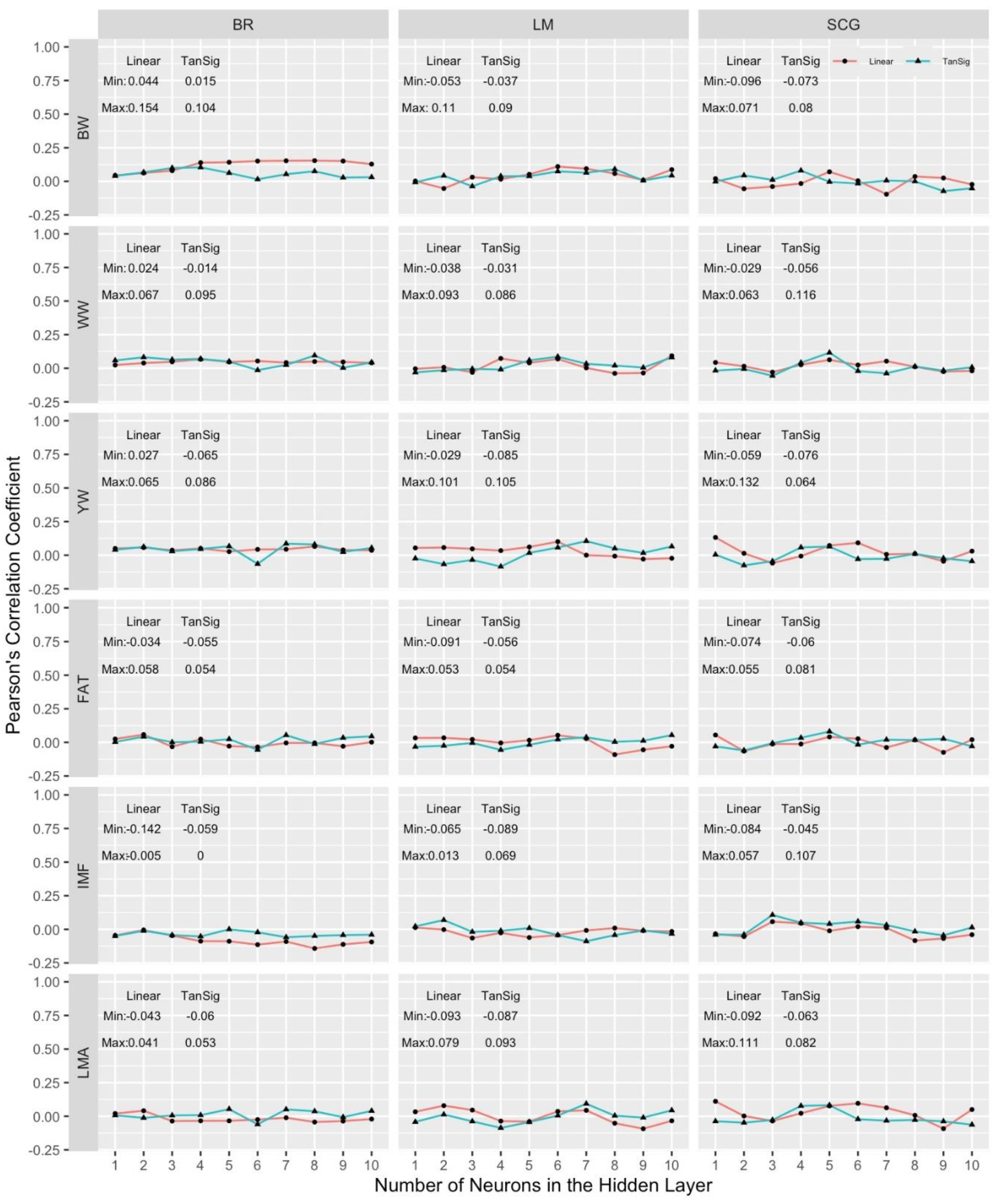
As seen in Figure 3 and Figure 4, Pearson’s correlation coefficients obtained for the predictive ability of MLPANN models ranged from -0.109 to 0.201 in the univariate analysis and from -0.142 to 0.154 in the multivariate analysis regardless of the growth and carcass traits, learning algorithms and transfer functions and the overall predictive ability of MLPANN models was low in the univariate and multivariate analysis of 10-fold cross-validation data sets. However, the predictive performances of MLPANN models in the univariate and multivariate analysis differed and paired-sample t-test showed that Pearson’s correlation coefficients from MLPANN models in the univariate analysis were statistically higher than those from MLPANN models in the multivariate analysis (p-value < 0.01).
The ranges of Pearson’s correlation coefficients from MLPANN models in the univariate analysis (Figure 3) were from -0.056 to 0.180 for BW, from -0.109 to 0.097 for WW, from -0.055 to 0.130 for YW, from -0.05 to 0.184 for FAT, from -0.041 to 0.201 for IMF and from -0.076 to 0.204 for LMA. Pearson’s correlation coefficients indicated that the predictive performances of MLPANN models for carcass traits were higher than those for growth traits. Peters et al. [31] carried out a simulation study to determine the genomic prediction performance of ANN models with 1 to 10 neurons using SNP markers in the analysis of two traits with heritabilities of 25% and 50% and results indicated that an increase in heritability resulted in an increase in the predictive performances of ANN models. Peters et al. [32] also analyzed the growth and carcass traits using GBLUP and Bayesian alphabet (BayesA, BayesB, BayesC and Bayesian Lasso) models and showed the predictive performances of GBLUP and Bayesian alphabet models by estimating the heritabilities of growth and carcass traits. The predictive performances of MLPANN models for growth and carcass traits were found lower than those of GBLUP and Bayesian alphabet (BayesA, BayesB, BayesC and Bayesian Lasso) models reported by Peters et al. [32]. However, Pearson’s correlation coefficients from MLPANN models in univariate analysis given in Figure 3 and those from GBLUP and Bayesian alphabet models in Peters et al. [32] for growth and carcass traits indicated that the carcass traits resulted in the higher predictive performances than growth traits since the carcass traits had the higher heritabilities than growth traits [32,33]. The effect of heritability of trait on genomic prediction in the comparison of different genomic models were studied by Daetwyler et al. [34] and Zhang et al. [35] and they indicated that genomic prediction models were sensitive to heritability and increasing heritability resulted in the increase in the predictive performance of genomic prediction models.
The ranges of Pearson’s correlation coefficients from MLPANN models in the multivariate analysis (Figure 4) were from -0.096 to 0.154 for BW, from -0.056 to 0.116 for WW, from -0.085 to 0.132 for YW, from -0.091 to 0.081 for FAT, from -0.142 to 0.107 for IMF and from -0.093 to 0.111 for LMA. Results from multivariate analysis were consistent with those from Peters et al. [36], who presented the predictive ability of MLPANN models in the multivariate analyses of growth (BW, WW and YW) traits based on the learning algorithms (BR, LM and SCG) and linear and tangent sigmoid transfer functions. In the ANN studies, network architecture, sample size in the training data set and the number of parameters (weights and biases) to be estimated are important factors effecting the predictive ability of MLPANN models. Okut et al. [37] showed that the number of parameters (weights and biases) were calculated by multiplying the number of inputs by the number of neurons in the MLPANN model in the univariate analysis. In this study, since the number of parameters in multivariate analysis were about 6 times larger than those in univariate analysis, the predictive ability of MLPANN models in multivariate analyses were found lower than that of MLPANN models in univariate analysis. Ether et al. [18] indicated that predictive ability of MLPANN models depended on network architecture when sample size was lower than the number of parameters in the analyses. In multivariate MLPANN models, as the number of neurons and the number of output increases, the number of parameters to be estimated also increases. Therefore, genomic relationship among animals could not provide enough information through input neurons to obtain high accuracy from multivariate MLPANN models.
Although the predictive ability of MLPANN models for carcass traits was better than those for growth traits in the univariate analysis, MLPANN models produced similar predictive ability for growth and carcass traits in the multivariate analysis which was resulted from the genetic relationship among traits. A genetic relationship between two traits happens when two traits are controlled in part by the same genes or linkage of the genes controlling the traits exists [38]. Results from the studies of Peters et al. [39], Rostamzadeh Mahdabi [40], Weik et al. [41] and Caetano et al. [42] indicated that most economically important traits such as growth (BW, WW and YW) and carcass (LMA, IMF and FAT) traits are genetically positively or negatively related and the degrees of relationship between them ranged from low to moderate. As seen in Figure 4, the complex MLPANN architecture (over 2 neurons in the hidden layer) in multivariate analysis attempted to learn specifications of the data and the underlying genetic relationships between traits could cause MLPANN models to learn irrelevant details of the data. Therefore, prediction performance of MLPANN models in multivariate analysis was substantially worse than that of MLPANN models in univariate analysis.
Comparison of learning algorithms and transfer functions for the predictive ability of MLPANN models
The predictive performance of MLPANN models depend upon the number of neurons in the hidden layer, learning algorithms and the type of transfer functions. Pearson’s correlation coefficients for the predictive performance of MLPANN models across the number of neurons are given for learning (BR, LM and SCG) algorithms and transfer (tangent sigmoid and linear) functions in Figure 3 for univariate analysis and in Figure 4 for multivariate analysis.
The predictive performance of MLPANN models was expected to show an increasing trend across the number of neurons in the hidden layer. However, as seen in Figure 3 and Figure 4, there were no increasing trends but fluctuations in the predictive performances of MLPANN models with increasing number of neurons across different learning algorithms and transfer functions in the univariate and multivariate analysis. There were also no specific number of neurons providing high predictive performance for MLPANN models in the univariate and multivariate analysis. These inconsistent predictive performance of MLPANN models indicated the necessity of many numbers of neurons to learn data specification in the applications of ANN. Okut et al. [37] comparing the predictive ability of different ANN-1-7-neuron models with BR learning algorithm indicated that the predictive ability of the network with five attained the highest Pearson’s correlation coefficient in the test data although differences among networks were negligible. Peters et al. [31] showed that predictive performance of MLPANN-1-10-neuron models increased with the number of neurons. However, there was no consistent increase in the predictive performance across the number of neurons, which indicated that a few numbers of neurons could not be enough to learn specification of data and could cause the under fitting problem. Although high number of neurons could be needed to learn relevant details of the data in the MLPANN applications, our MLPANN predictive performance results in Figure 3 and Figure 4 were also found similar across the number of neurons in the univariate and multivariate analysis of growth and carcass traits. Ehret et al [18], Gianola et al. [43] and Sinecen [44] showed that the ANN models differed little in predictive performance across the number of neurons when the genomic relationship G matrix was used. Peters et al. [31] indicated that ANN predictive performance agreed when the sample size was equal to or higher than the number of features of the network.
In this study, BR, LM and SCG backpropagation learning algorithms were used to determine the MLPANN learning algorithm producing better estimates in the univariate and multivariate analyses of growth and carcass traits. Pearson’s correlation coefficients from MLPANN models with BR, LM and SCG learning algorithms were given in columns within Figure 3 and Figure 4 to determine the learning algorithm producing better estimates in the univariate and multivariate analyses of growth and carcass traits. As seen in Figure 3 and Figure 4, Pearson’s correlation coefficients ranged from 0.024 to 0.204 for BR, from -0.052 to 0.184 for LM and from -0.109 to 0.147 for SCG learning algorithms in the univariate analysis; ranged from -0.142 to 0.154 for BR, from -0.093 to 0.110 for LM and from -0.096 to 0.132 for SCG learning algorithms in the multivariate analysis, respectively. These results indicated that the predictive performances of BR, LM and SCG learning algorithms in the univariate analysis were different than those in the multivariate analysis.
In the univariate analysis, MLPANN models with BR learning algorithm resulted in better predictive performances compared with MLPANN models with LM and SCG algorithms. Also, more consistent predictive performances of MLPANN models across the number of neurons were obtained in the BR learning algorithm. Results from the BR learning algorithm are consistent with those of Okut et al. [37], who demonstrated that predictive performance of ANN models did not depend on network architecture when sample size was larger than the number of features in the analysis. Our results also agreed with those of Ehret et al. [18] who used the G matrix as input to the network and those of Gianola et al. [43], who used Bayesian regularized artificial networks for genome-enabled predictions of milk traits in Jersey cows. Peters et al. [45] compared the MLPANN models with BR, LM and SCG learning algorithms for the analysis of antler beam diameter and length from white-tailed deer and found that MLPANN model with BR learning algorithm showed better agreement of the predicted and observed values of antler beam diameter and length; however, MLPANN model with SCG learning algorithm resulted in the highest error within the models. Kayri [46] compared ANN models with BR and LM learning algorithms in the analysis of social data and found that BR learning algorithm with the higher Pearson’s correlation coefficient indicated better predictive performance than LM learning algorithm. Okut et al. [47] investigated the predictive performance of BR and SCG learning algorithms and found that the ANN model with BR learning algorithm gave slightly better performance. In the studies of Bruneau and McElroy [48], Saini [49], Laurent et al. [50] and Ticknor [51], the BR learning algorithm also yielded moderate or better predictive performance compared with the other learning algorithms.
ANN models were usually applied in the univariate analysis and resulted in similar and consistent predictive performances across learning algorithms and transfer functions [18,45,47]. However, as seen in Figure 4, Pearson’s correlation coefficients from the multivariate analysis indicated that predictive performances of MLPANN models with BR, LM and SCG learning algorithms were different, not consistent across growth and carcass traits, the number of neurons and transfer functions and not better than those from the univariate analysis. Training in the ANN model is an iterative learning process and at each iteration the weights from input to hidden layer () and from hidden to output layer () of the ANN model (Figure 1) are adjusted by using a learning algorithm (BR, LM and SCG) [18] to minimize the difference (the error) between observed and predicted phenotypes [52]. Since six growth (BW, WW and YW) and carcass (FAT, IMF and LMA) traits were analyzed together by using the MLPANN models with BR, LM and SCG learning algorithms in the multivariate analysis, the increasing number of features of the MLPANN model and the underlying (positive/negative) genetic relationships among traits affected the iterative learning process of BR, LM and SCG learning algorithms within neural network and resulted in lower predictive performance of the MLPANN models with BR, LM and SCG learning algorithms in the multivariate analysis.
Transfer function is an essential part of ANN model to help in learning and making sense of non-linear and complicated mappings between the inputs (genomic relationship) and corresponding outputs (the value of trait or phenotype) [53]. Applying a sigmoidal-type and linear transfer functions in the hidden and output layers may be useful when it is necessary to extrapolate beyond the range of the training data [54]. In this study, two combinations of transfer functions (tangent sigmoid-linear and linear-linear) were used in the hidden-output layers (Figure 1). For predictive performances of MLPANN models with tangent sigmoid-linear or linear-linear transfer function combination, minimum and maximum values of Pearson’s correlation coefficients for the tangent sigmoid-linear or linear-linear transfer function combination were given based on growth and carcass traits and BR, LM and SCG learning algorithms in univariate (Figure 3) and multivariate (Figure 4) analyses. As seen in Figure 3 and Figure 4, Pearson’s correlation coefficients indicated that predictive performances of MLPANN models with tangent sigmoid-linear or linear-linear transfer function combination in univariate analysis were better than those in multivariate analysis. In addition, predictive performances of tangent sigmoid-linear and linear-linear transfer function combinations within univariate and multivariate analyses were different across growth and carcass traits and BR, LM and SCG learning algorithms.
In univariate analysis, predictive performances of MLPANN models with tangent sigmoid-linear transfer function combination for each trait were better than or similar with those of MLPANN models with linear-linear transfer function combination across learning algorithms. MLPANN models with tangent sigmoid-linear or linear-linear transfer function combination in BR learning algorithm resulted in higher predictive performances than those in LM and SCG learning algorithms. Also, predictive performances of transfer function combinations were more consistent in BR learning algorithm compared with those in LM and SCG learning algorithms. However, in multivariate analysis, MLPANN models with tangent sigmoid-linear or linear-linear transfer function combination in BR learning algorithm yielded lower predictive performances than those in LM and SCG learning algorithms and tangent sigmoid-linear and linear-linear transfer function combinations in BR learning algorithm resulted in the worst predictive performances for carcass traits of FAT, IMF and LMA and the overall predictive performance of transfer function combinations in LM and SCG learning algorithms were better than those in BR learning algorithm. As indicated by Ehret et al. [18], the complex architectures of MLPANN models and the underlying genetic relationships among growth and carcass traits in the multivariate analysis could cause worse predictive performances by learning irrelevant details of the data.
4. Conclusions
The results from this study showed that MLPANN-1-10-neuron models with the BR, LM and SCG learning algorithms based on the tangent sigmoid-linear and linear-linear transfer function combinations in the univariate analysis of growth and carcass traits resulted in better predictive performances than those in the multivariate analysis. In the univariate analysis, MLPANN-1-10-neuron models with BR learning algorithm based on the tangent sigmoid-linear or linear-linear transfer function combination yielded higher predictive performances than those in LM and SCG learning algorithms. In addition, predictive performances of MLPANN models with tangent sigmoid-linear transfer function combination were better than those with linear-linear transfer function combination in the univariate analysis. The complex architectures of MLPANN models and genetic relationship among growth and carcass traits in the multivariate analysis could affect the predictive performances of BR, LM and SCG learning algorithms and the tangent sigmoid-linear and linear-linear transfer function combinations.
Author Contributions
Conceptualization, S.O.P., K.K., M.S and M.G.T.; data curation, S.O.P., M.G.T. and K.K.; methodology, S.O.P., K.K. and M.S.; software, M.S.; formal analysis, M.S.; validation, K.K. and M.S.; writing—original draft preparation, S.O.P and K.K.; writing—review and editing, S.O.P., K.K., M.S. and M.G.T.
Funding
Financial support provided by USDA-AFRI (Grant no. 2008-35205- 18751 and 2009-35205-05100) and New Mexico Agric. Exp. Stan. Project (Hatch#216391). Collaboration developed from activities of National Beef Cattle Evaluation Consortium. Authors acknowledge Camp Cooley Ranch (Franklin, TX) for supplying DNA and phenotypes from Brangus heifers, and Robert Schnabel, University of Missouri, for providing SNP information for BovineSNP50.
Data Availability Statement
The datasets analysed during the current study are available for academic purposes upon signing a Material Transfer Agreement with the corresponding author (speters@berry.edu).
Conflicts of Interest
The authors declare no conflict of interest.
References
- Meuwissen, T.H.E.; Hayes, B.J.; Goddard, M.E. Prediction of total genetic value using genome-wide dense marker maps. Genetics 2001, 157, 1819–1829. [Google Scholar] [CrossRef] [PubMed]
- Matukumalli, L.K.; Lawley, C.T.; Schnabel, R.D.; Taylor, J.F.; Allan, M.F.; Heaton, M.P.; O’Connell, J.; Moore, S.S.; Smith, T.P.L.; Sonstegard, T.S.; Van Tassell, C.P. Development and characterization of high density SNP genotyping assay for cattle. PLoS ONE 2009, 4, e5350. [Google Scholar] [CrossRef] [PubMed]
- Applied Biosystems. Axiom Bovine Genotyping v3 Array (384HT format). 2019. Available online: https://www.thermofisher.com/order/catalog/product/55108%209#/551089 (accessed on 15 January 2022).
- Illumina. Infinium iSelect Custom Genotyping Assays. 2016. Available online: https://www.illumina.com/content/dam/illumina-marketing/documents/products/technotes/technote_iselect_design.pdf (accessed on 15 January 2022).
- Habier, D.; Fernando, R.L.; Kizilkaya, K.; Garrick, D.J. Extension of the Bayesian alphabet for genomic selection. BMC Bioinform. 2011, 12, 186. [Google Scholar] [CrossRef] [PubMed]
- Pérez, P.; de los Campos, G. Genome-wide regression and prediction with the BGLR statistical package. Genetics 2014, 198, 483–495. [Google Scholar] [CrossRef]
- de Pereira, B.B.; Rao, C.R.; Rao, M. Data Mining using Neural Networks: A Guide for Statistician, 1st ed.; Chapman and Hall/CRC, 2009. [Google Scholar]
- Kononenko, I.; Kukar, M. Machine Learning and Data Mining: Introduction to Principles and Algorithms; Horwood Publishing: London, 2007. [Google Scholar]
- Howard, R.; Carriquiry, A.L.; and Beavis, W.D. Parametric and Nonparametric Statistical Methods for Genomic Selection of Traits with Additive and Epistatic Genetic Architectures. G3 Genes|Genomes|Genetics 2024, 4, 1027–1046. [Google Scholar] [CrossRef]
- Luna-Nevarez, P.; Bailey, D.W.; Bailey, C.C.; VanLeeuwen, D.M.; Enns, R.M.; Silver, G.A.; DeAtley, K.L.; Thomas, M.G. Growth characteristics, reproductive performance, and evaluation of their associative relationships in Brangus cattle managed in a Chihuahuan Desert production system. J Anim Sci 2010, 88, 1891–1904. [Google Scholar] [CrossRef]
- Fortes, M.R.S.; Snelling, W.M.; Reverter, A.; Nagaraji, S.H.; Lehnert, S.A.; Hawken, R.J.; DeAtley, K.L.; Peters, S.O.; Silver, G.A.; Rincon, G.; Medrano, J.F.; Isla-Trejo, A.; Thomas, M.G. Gene network analyses of first service conception in Brangus heifers: Use of genome and trait associations, hypothalamic-transcriptome information, and transcription factors. J. Anim. Sci. 2012, 90, 2894–2906. [Google Scholar] [CrossRef]
- Peters, S.O.; Kizilkaya, K.; Garrick, D.J.; Fernando, R.L.; Reecy, J.M.; Weaber, R.L.; Silver, G.A.; Thomas, M.G. Bayesian genome-wide association analysis of growth and yearling ultrasound measures of carcass traits in Brangus heifers. J. Anim. Sci. 2012, 90, 3398–3409. [Google Scholar] [CrossRef]
- Granato, I.S.C.; Galli, G.; de Oliveira Couto, E.G.; et al. snpReady: a tool to assist breeders in genomic analysis. Mol Breeding 2018, 38, 102. [Google Scholar] [CrossRef]
- Habier, D.; Fernando, R.L.; Dekkers, J.C.M. The impact of genetic relationship information on genome-assisted breeding values. Genetics 2007, 177, 2389–2397. [Google Scholar] [CrossRef]
- vanRaden, P.M. Efficient methods to compute genomic predictions. J. Dairy Sci. 2008, 91, 4414–4423. [Google Scholar] [CrossRef] [PubMed]
- Cybenko, G. Approximation by superpositions of a sigmoidal function. Math Control Signals, Syst. 1989, 2, 303–314. [Google Scholar] [CrossRef]
- Hornik, K.; Stinchcombe, M.; White, H. Multilayer feedforward networks are universal approximators. Neural Networks 1989, 2, 359–366. [Google Scholar] [CrossRef]
- Ehret, A.; Hochstuhl, D.; Gianola, D.; Thaller, G. Application of neural networks with back-propagation to genome-enabled prediction of complex traits in Holstein-Friesian and German Fleckvieh cattle. Genet Sel Evol. 2015, 47, 22. [Google Scholar] [CrossRef] [PubMed]
- Haykin, S.S. Neural networks: a comprehensive foundation; Prentice Hall, 1999; 842p. [Google Scholar]
- Kröse, B.; Smagt Patrick, V.D. An introduction to Neural Networks, 8th ed.; The University of Amsterdam: Amsterdam, 1996; 135p. [Google Scholar]
- Christodoulou, C.G.; Georgiopoulos, M. Applications of neural networks in electromagnetics, 1st ed.; Artech House: Norwood, 2001; 512p. [Google Scholar]
- Civco, D.L. Artificial neural networks for land cover classification and mapping. International Journal of Geographical Information Systems 1993, 7, 173–186. [Google Scholar] [CrossRef]
- Kaminsky, E.J.; Barad, H.; Brown, W. Textural neural network and version space classifiers for remote sensing. International Journal of Remote Sensing 1997, 18, 741–762. [Google Scholar] [CrossRef]
- Bouabaz, M.; Hamami, M. A Cost Estimation Model for Repair Bridges Based on Artificial Neural Network. American Journal of Applied Sciences 2008, 5. [Google Scholar] [CrossRef]
- Dorofki, M.; Elshafie, A.; Jaafar, O.; A Karim, O.; Mastura, S. Comparison of Artificial Neural Network Transfer Functions Abilities to Simulate Extreme Runoff Data. Int Proc Chem Biol Environ Eng. 2012, 33. [Google Scholar]
- Saatchi, M.; McClure, M.C.; McKay, S.D.; Rolf, M.M.; Kim, J.; Decker, J.E.; Taxis, T.M.; Chapple, R.H.; Ramey, H.R.; Northcutt, S.L.; Bauck, S.; Woodward, B.; Dekkers, J.C.M.; Fernando, R.L.; Schnabel, R.D.; Garrick, D.J.; Taylor, J.F. Accuracies of genomic breeding values in American Angus beef cattle using K-means clustering for cross-validation. Genet. Sel. Evol. 2011, 43, 40. [Google Scholar] [CrossRef]
- Hartigan, J.A.; Wong, M.A.; Algorithm, A.S. 136: A k-means clustering algorithm. Appl. Stat. 1979, 28, 100–108. [Google Scholar] [CrossRef]
- Gorjanc, G.; Henderson, D.A.; Kinghorn, B.; Percy, A. GeneticsPed: Pedigree and genetic relationship functions. R package version 1.52.0. 2020. Available online: http://rgenetics.org.
- Kassambara, A.; Mundt, F. factoextra: Extract and Visualize the Results of Multivariate Data Analyses. R package version 1.0.5. 2017. Available online: https://CRAN.R-project.org/package=factoextra.
- Demuth, H.; Beale, M. Neural Network Toolbox User's Guide; The Mathworks: Natick, 2000. [Google Scholar]
- Peters, S.; Sinecen, M.; Kizilkaya, K.; Thomas, M. Genomic prediction with different heritability, QTL and SNP panel scenarios using artificial neural network. IEEE Access 2020, 1. [Google Scholar] [CrossRef]
- Peters, S.O.; Kizilkaya, K.; Sinecen, M.; Metav, B.; Thiruvenkadan, A.K.; Thomas, M.G. Genomic Prediction Accuracies for Growth and Carcass Traits in a Brangus Heifer Population. Animals 2023, 13, 1272. [Google Scholar] [CrossRef] [PubMed]
- Peters, S.O.; Kizilkaya, K.; Garrick, D.J.; Fernando, R.L.; Reecy, J.M.; Weaber, R.L.; Silver, G.A.; Thomas, M.G. Bayesian QTL inference from whole genome analysis of growth and composition in yearling Brangus heifers. J. Anim. Sci. 2012, 90, 3398–3409. [Google Scholar] [CrossRef] [PubMed]
- Daetwyler, H.D.; Pong-Wong, R.; Villanueva, B.; Woolliams, J.A. The impact of genetic architecture on genome-wide evaluation methods. Genetics 2010, 185, 1021–1031. [Google Scholar] [CrossRef]
- Zhang, Z.; Liu, J.; Ding, X.; Bijma, P.; de Koning, D.-J.; Zhang, Q. ‘Best linear unbiased prediction of genomic breeding values using a trait-specific marker-derived relationship matrix. PLoS ONE 2010, 5, e12648. [Google Scholar] [CrossRef]
- Peters, S.O.; Kizilkaya, K.; Sinecen, M.; Thomas, M.G. Multivariate Application of Artificial Neural Networks for Genomic Prediction. World Congress on Genetics Applied to Livestock Production, Rotterdam, Netherlands, 3-8 July 2022.
- Okut, H.; Gianola, D.; Rosa, G.J.M.; Weigel, K.A. Prediction of body mass index in mice using dense molecular markers and a regularized neural network. Genet. Res. 2011, 93, 189–201. [Google Scholar] [CrossRef]
- Herring, W. What have we learned about trait relationships. 2003, 1-8. Available online: https://animal.ifas.ufl.edu/beef_extension/bcsc/2002/pdf/herring.
- Peters, S.O.; Kizilkaya, K.; Garrick, D.; Reecy, J. PSX-9 Comparison of single- and multiple-trait genomic predictions of cattle carcass quality traits in multibreed and purebred populations. J. Anim. Sci. 2024, 102, 453–454. [Google Scholar] [CrossRef]
- Rostamzadeh Mahdabi, E.; Tian, R.; Li, Y.; Wang, X.; Zhao, M.; Li, H.; Yang, D.; Zhang, H.; Li, S.; Esmailizadeh, A. Genomic heritability and correlation between carcass traits in Japanese Black cattle evaluated under different ceilings of relatedness among individuals. Front. Genet. 2023, 14, 1053291. [Google Scholar] [CrossRef]
- Weik, F.; Hickson, R.E.; Morris, S.T.; Garrick, D.J.; Archer, J.A. Genetic Parameters for Growth, Ultrasound and Carcass Traits in New Zealand Beef Cattle and Their Correlations with Maternal Performance. Animals 2022, 12, 25. [Google Scholar] [CrossRef]
- Caetano, S.L.; Savegnago, R.P.; Boligon, A.A.; Ramos, S.B.; Chud, T.C.S.; Lôbo, R.B.; Munari, D.P. Estimates of genetic parameters for carcass, growth and reproductive traits in Nellore cattle. Livestock Science 2013, 155, 1–7. [Google Scholar] [CrossRef]
- Gianola, D.; Okut, H.; Weigel, K.; Rosa, G. Predicting complex quantitative traits with Bayesian neural networks: a case study with Jersey cows and wheat. BMC Genetics 2011, 12, 87. [Google Scholar] [CrossRef] [PubMed]
- Sinecen, M. Comparison of genomic best linear unbiased prediction and Bayesian regularization neural networks for genomic selection. IEEE Access 2019, 7, 79199–79210. [Google Scholar] [CrossRef]
- Peters, S.O.; Sinecen, M.; Gallagher, G.R.; Lauren, A.P.; Jacob, S.; Hatfield, J.S.; Kizilkaya, K. Comparison Of Linear Model And Artificial Neural Network Using Antler Beam Diameter And Length Of White-Tailed Deer (Odocoileus Virginianus) Dataset. Plos One 2019, 14, 1–14. [Google Scholar] [CrossRef] [PubMed]
- Kayri, M. Predictive Abilities of Bayesian Regularization and LevenbergMarquardt Algorithms in Artificial Neural Networks: A Comparative Empirical Study on Social Data. Math. Comput. Appl. 2016, 21, 20. [Google Scholar] [CrossRef]
- Okut, H.; Wu, X.L.; Rosa, G.J.M.; Bauck, S.; Woodward, B.W.; Schnabel, R.D.; Taylor, J.F.; Gianola, D. Predicting expected progeny difference for marbling score in Angus cattle using artificial neural networks and Bayesian regression models. Genet. Sel. Evolut. 2013, 45, 1–8. [Google Scholar] [CrossRef]
- Bruneau, P.; McElroy, N.R. LogD7.4 modeling using Bayesian regularized neural networks assessment and correction of the errors of prediction. J. Chem. Inf. Model. 2006, 46, 1379–1387. [Google Scholar] [CrossRef]
- Saini, L.M. Peak load forecasting using Bayesian regularization, Resilient and adaptive backpropagation learning based artificial neural networks. Electr. Power Syst. Res. 2008, 78, 1302–1310. [Google Scholar] [CrossRef]
- Lauret, P.; Fock, F.; Randrianarivony, R.N.; Manicom-Ramsamy, J.F. Bayesian Neural Network approach to short time load forecasting. Energy Convers. Manag. 2008, 5, 1156–1166. [Google Scholar] [CrossRef]
- Ticknor, J.L. A Bayesian regularized artificial neural network for stock market forecasting. Expert Syst. Appl. 2013, 14, 5501–5506. [Google Scholar] [CrossRef]
- Gurney, K.; Burney, K. An introduction to neural networks; 1997; Volume 1. [Google Scholar]
- Sharma, S.; Sharma, S.; Athaiya, A. Activation functions in neural networks. International Journal of Engineering Applied Sciences and Technology 2020, 4, 310–316. [Google Scholar] [CrossRef]
- Maier, H.R.; Dandy, C.G. Neural networks for the prediction and forecasting of water resources variables: a review of modelling issues and applications. Environmental Modelling and Software 2000, 15, 101–124. [Google Scholar] [CrossRef]
Figure 1.
Graphical representation of the univariate and multivariate multi-layer perceptron artificial neural networks for the inputs of the additive genomic relationships () between animals from G Matrix and the output of the univariate () or multivariate () predicted values of phenotypes () by the network where .
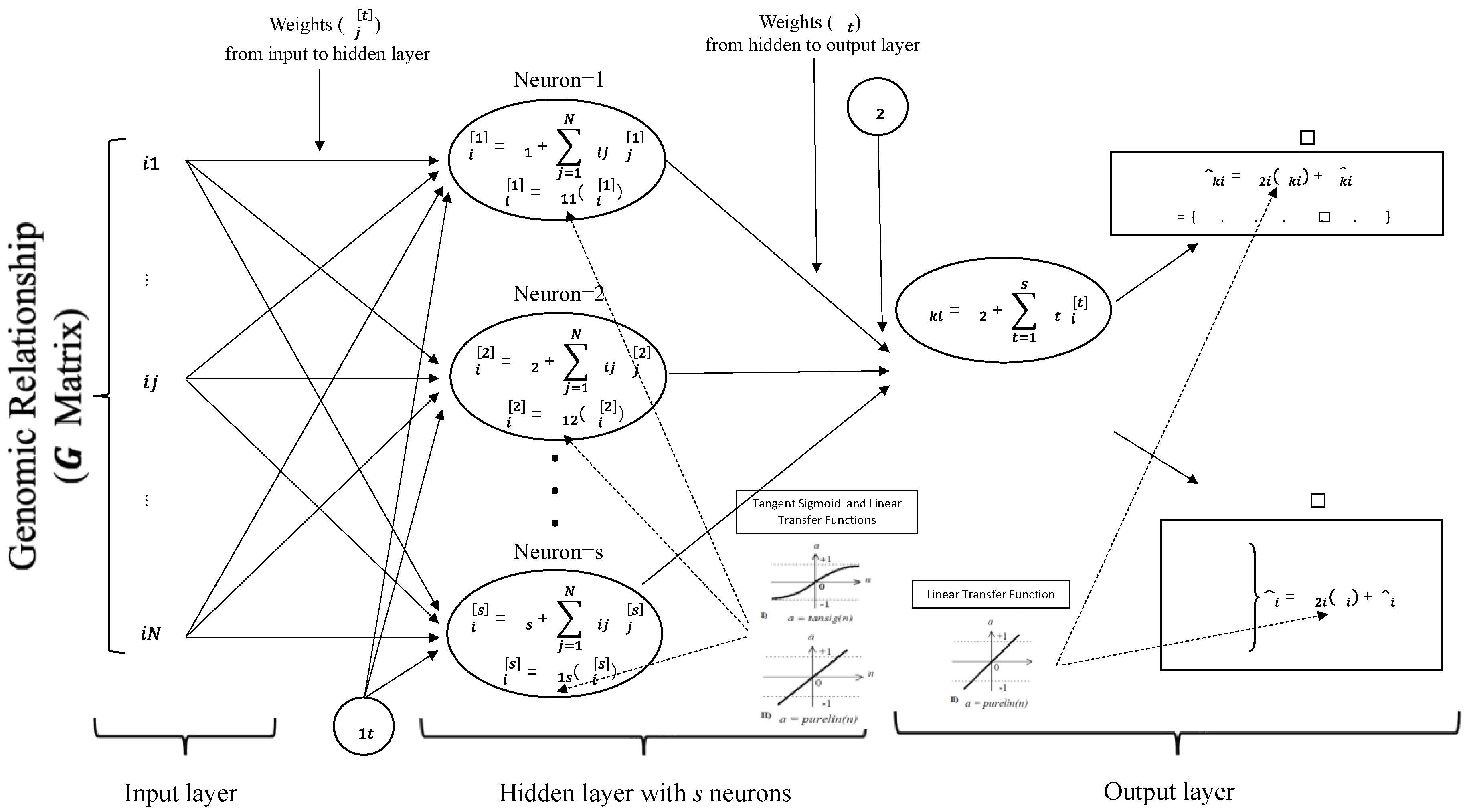
Figure 2.
Tangent sigmoid and linear transfer functions in the hidden during the training process in the MLPANN model.
Figure 2.
Tangent sigmoid and linear transfer functions in the hidden during the training process in the MLPANN model.
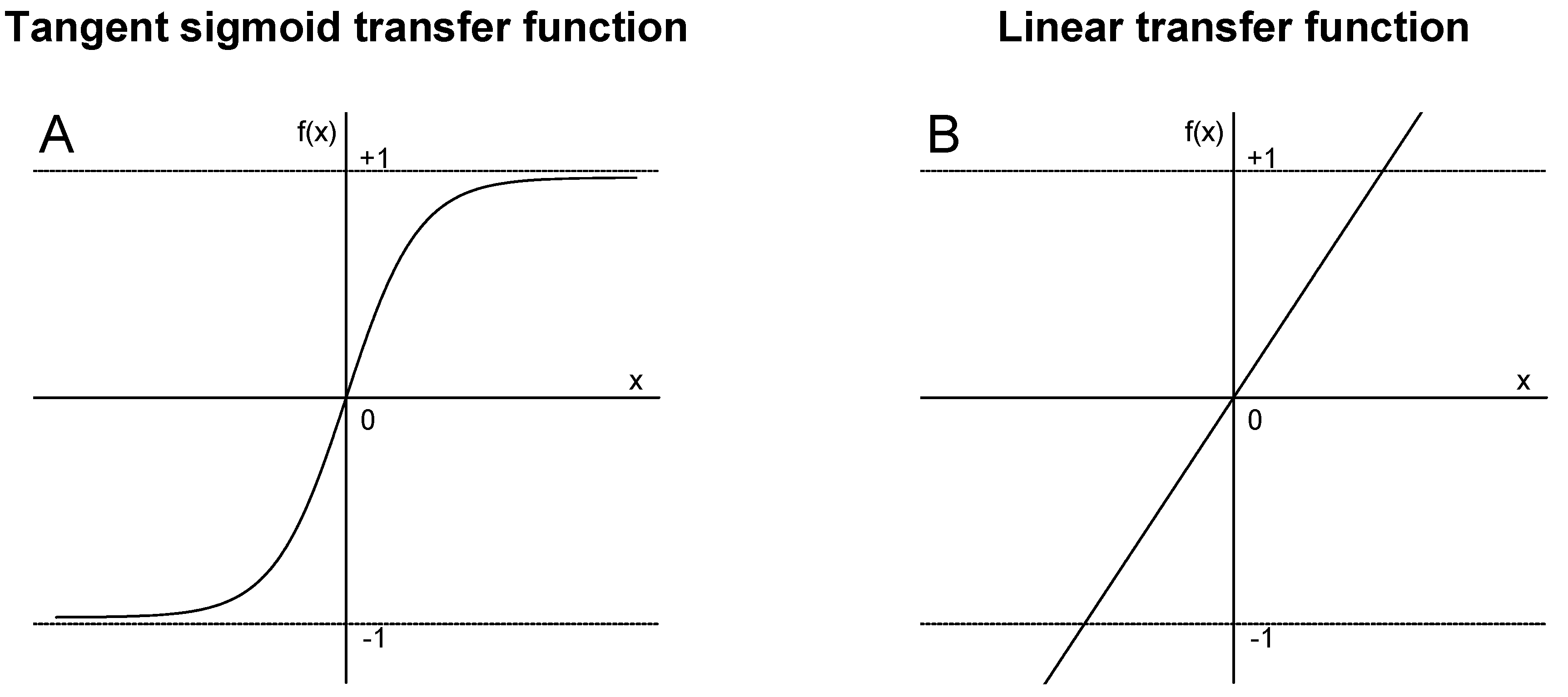
Figure 3.
Comparison of predictive abilities for all scenarios in MLPANN model structure using univariate validation data sets. Growth (BW, WW and YW) and carcass (LMA, IMF and FAT) traits are in the rows, in columns BR, LM and SCG learning algorithms are shown. Panels show the average Pearson’s correlation coefficients over univariate validation data sets in 10 cross-validation runs on the vertical axis, and the number of neurons tested on the horizontal axis. Results of linear-linear (Linear) and tangent sigmoid-linear (TanSig) transfer function combinations are presented in each panel.
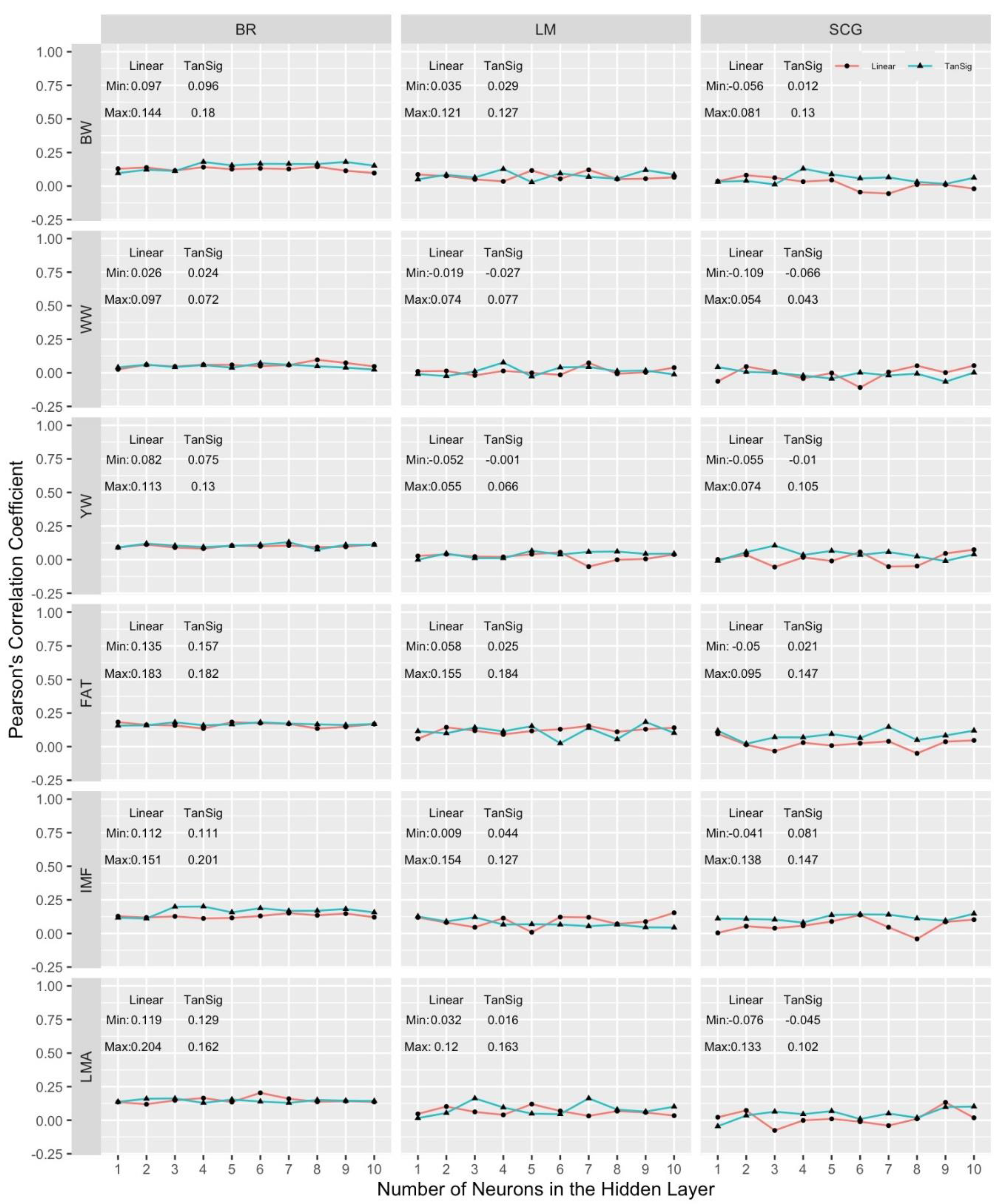
Figure 4.
Comparison of predictive abilities for all scenarios in MLPANN model structure using multivariate validation data sets. Growth (BW, WW and YW) and carcass (LMA, IMF and FAT) traits are in the rows, in columns BR, LM and SCG learning algorithms are shown. Panels show the average Pearson’s correlation coefficients over multivariate validation data sets in 10 cross-validation runs on the vertical axis, and the number of neurons tested on the horizontal axis. Results of linear-linear (Linear) and tangent sigmoid-linear (TanSig) transfer function combinations are presented in each panel.
Disclaimer/Publisher’s Note: The statements, opinions and data contained in all publications are solely those of the individual author(s) and contributor(s) and not of MDPI and/or the editor(s). MDPI and/or the editor(s) disclaim responsibility for any injury to people or property resulting from any ideas, methods, instructions or products referred to in the content. |
© 2025 by the authors. Licensee MDPI, Basel, Switzerland. This article is an open access article distributed under the terms and conditions of the Creative Commons Attribution (CC BY) license (http://creativecommons.org/licenses/by/4.0/).
Copyright: This open access article is published under a Creative Commons CC BY 4.0 license, which permit the free download, distribution, and reuse, provided that the author and preprint are cited in any reuse.


