Characteristics and Optimization of Transient Process of Pump Turbine Units in Power Generation Mode

1. Introduction

With the rapid development of clean energy sources such as nuclear, wind, and solar energy [1], supporting energy storage facilities are required due to their weak regulation ability. In general, battery energy storage [2], compressed air energy storage [3], and flywheel energy storage [4] are good options, but the pumped storage power stations (PSPSs) are consensual the most mature and large-scale ideal regulated power sources [5,6,7]. Therefore, the Chinese mainland is vigorously developing the pumped storage technology. By the end of 2023, the installed capacity of the PSPSs under construction in China reached 167 million kW, and it is expected to reach 300 million kW by 2035 [8].

The PSPSs play the roles of frequency regulation, peak load shaving, and emergency power supply in the power grid [9,10]. To accomplish above tasks, the pump-turbines (PTs) need to constantly go through various transient processes between start up and shutdown, which poses a challenge to the safe and stable operation of the PTs. The no-load instability is a typical operating problem of the PT. Zhao et al. studied the no-load operational dynamic characteristic by bifurcation diagram, and analyzed the no-load stability of the PT by introducing step disturbance and slopes. They found that different disturbance intensity and slopes have different influence on no-load stability [11]. Sun et al. investigated the effect of misaligned guide vanes (MGVs) to control the stability in the S region, they found that the MGVs can improve the no-load stability, but intensify pressure fluctuation [12]. During the start-up transient process in the power generation mode, due to the large variations of the parameters such as discharge, water head, the vibration of the pump-turbine unit (PTU) will inevitably be intensified, which threaten the safe operation of the PTU. Yang et al. studied the flow-induced vibration of the PTU by three-dimensional CFD technology, and believed that it is strongly related to the axial thrust caused by the fluid flow [13]. Emphatically, there are a large amount of research literatures to focus water hammer pressure and pulsating pressure during the transient process of load rejection. Zeng et al. developed a simplified mathematical model of transient process, derived the analytical expression for the change rate of water head, and discussed the relationship between the trajectory slopes in different domains and water-hammer pressure, and optimized the guide-vane closure schemes for reducing the maximum transient pressure.They believe that the three-phase valve-closing schemes has advantages in controlling pulsating pressure and runaway velocity [14]. Zhao et al. proposed a novel optimization framework to derive optimal operating policies for pumped storage hydropower system. The results shown that the maximum water pressure of volute and the vacuum at draft tube can be improved by 5.59% and 9.6%, and the rotational speed oscillation also be decreased, compared with the on-site operation [15]. Ye et al. developed a water hammer pressure model combined with genetic algorithms or non-dominated sorting genetic algorithm II, and optimized the closure schemes for the guide vanes of the PT and ball valve. The result shown that pressure coefficient in the pump turbine is reduced. However, due to the error of the peak-to-peak diagrams, the estimated fluctuating pressure in the proposed model is inevitably biased, and this method needs to be improved [16]. Zhang et al. formulated a dynamic model of the PT by introducing a stochastic variable, investigated the stochastic dynamic characteristics of the PT in load-rejection process, and analyzed the effects of the stochastic intensity on the dynamic behavior of the PT. The result shown that pressure coefficient in the pump turbine is reduced. However, due to the error of the peak-to-peak diagrams, the estimated fluctuating pressure in the proposed model is inevitably biased, and this method needs to be improved [17].

In short, more scholars are focused on the study of transient process of load rejection. In fact, the optimization of the entire transient processes of the PTUs in the power generation mode is also worthy of in-depth study. Compared with conventional hydropower plants, the PSPS has a small reservoir capacity leading to large variation of water head, coupled with the reverse “S” characteristics of the PT, so the operation stability of the PTU is poor, and the load regulation is slow, which affect the operation safety of the PTU [18,19]. Traditionally, the characteristic method is commonly used in hydraulic transition process calculations [17,20]. However, this method is difficult to capture the pulsating pressure of the transition process. In this paper, taking a “one diversion tunnel with two PTUs” as an example, a hydraulic-mechanical-electrical coupling model is constructed, a variable-time-step Euler algorithm is presented and the method of peak staggering and valley filling is used to calculate the appropriate peak staggering regulation time and optimize the closure law of the guide vanes to improve the characteristics of the transient process of the PTU and ensure the power quality.

The rest of this paper is organized as follows. In section 2, the mathematical model of pump turbine regulation system and the project overview of a typical PSPS are introduced. Then three typical transient processes are calculated and optimized in section 3. Finally, conclusions are summarized in section 4.

2. Model of Pump Turbine Regulation System

2.1. Model of Diversion Pipeline

2.1.1. Elastic Water Hammer Model

The diversion pipeline is composed of the diversion tunnel, pressure pipe, tailwater pipeline and tailwater tunnel. The elastic water hammer model of diversion pipeline is described by the following continuity and momentum equations:

$$\partial H/\partial t+V\partial H/\partial x+k_1\partial Q/\partial x=0$$

(1)

$$\partial Q/\partial t+V\partial Q/\partial x+k_2\partial H/\partial x+k_3\left|Q\right|Q=0$$

(2)

where, $H$ is water head, m; $Q$ is discharge, m³/s; $V$ is flow velocity, m/s; $t$ is time, s; the coefficients $k_1=a^2/gS$, $k_2=gS,k_3=f/2DS$; $a$ is water hammer wave speed, m/s；$g$ is the gravitational acceleration, m²/s；$f$ is the Darcy-Weisbach friction factor; $S$ is the section area of pipeline, m²; $D$ is the dimeter of pipeline, m.

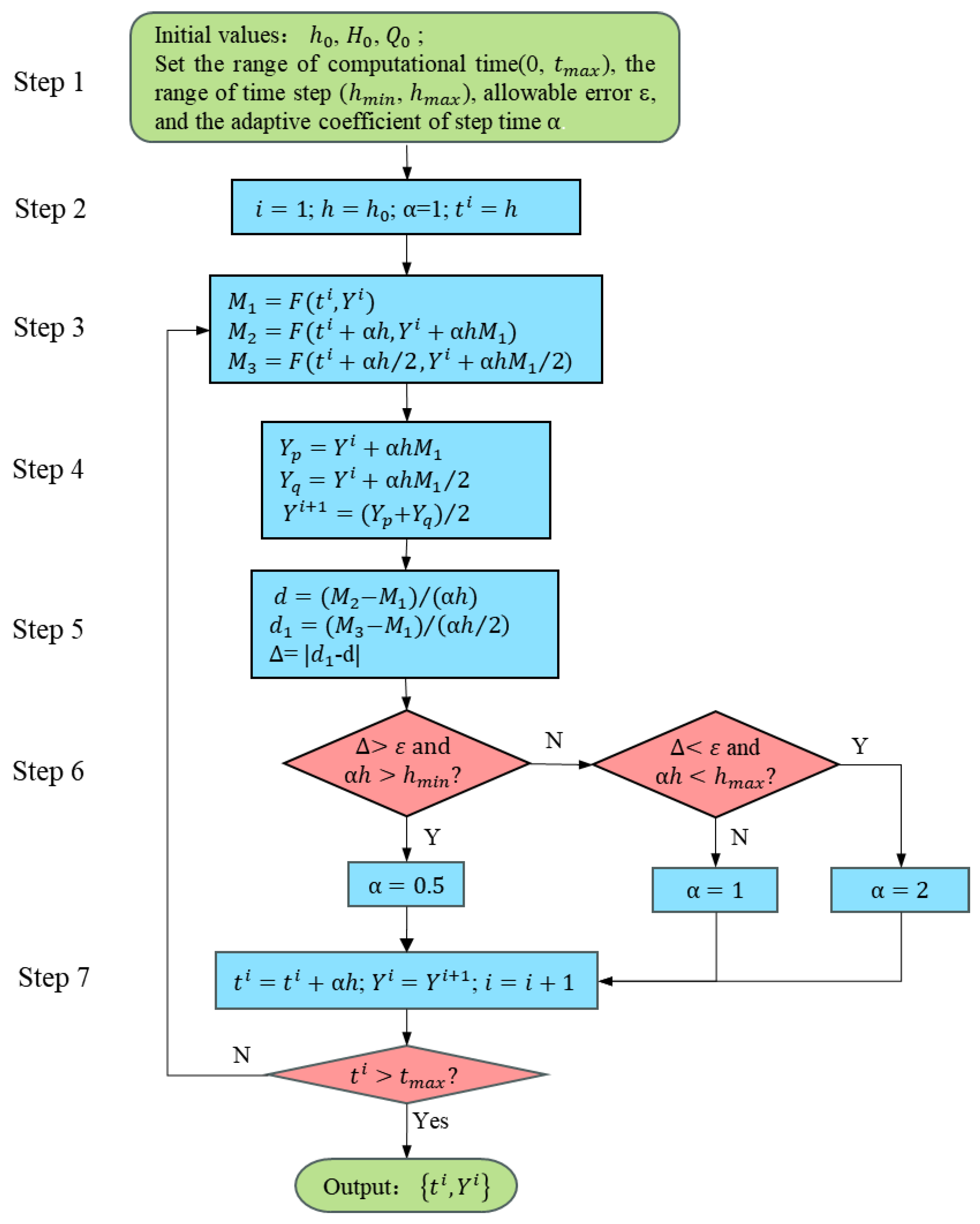
2.1.2. Algorithm of Hydraulic Transient Process

Equations (1) and (2) can be converted into the problem of the initial values of differential equations.

$$\left\{\begin{array}{c}dH/dt=-k_1\partial Q/\partial x\\ H_0=H\left(t_0\right)\end{array}\right.$$

(3)

$$\left\{\begin{array}{c}dQ/dt=-k_2\partial H/\partial x-k_3\left|Q\right|Q\\ Q_0=Q\left(t_0\right)\end{array}\right.$$

(4)

Generally, Equations (3) and (4) can be expressed in a generic form:

$$\dot{Y}=F(t,Y)$$

(5)

where, variable is $Y={\left(H,Q\right)}^T$, function is $F\left(t,Y\right)={\left(-k_1\partial Q/\partial x,-k_2\partial H/\partial x-k_3\left|Q\right|Q\right)}^T$.

In this section, a variable-time-step Euler algorithm is presented, the flowchart is shown in Figure 1.

Firstly, give the initial values: initial time step ($h_0$), initial water head ($H_0$), initial discharge ($Q_0$), and set the range of computational time(0, $t_{max}$), the range of time step ($h_{min}$, $h_{max}$), allowable error ε, and the adaptive coefficient of step time$\alpha$. Step 2: set time step is equal to $h_0$, the adaptive coefficient of time step$\alpha$=1, and computational time $t^i=h$. Step 3: Calculate intermediate functions $M_1$, $M_2$ and $M_3$. Step 4: Modified Euler method is used to calculate $Y^{i+1}$. Step 5: Define the solution error Δ. Step 6: Solve the adaptive coefficient of step time$\alpha$, if the error Δ is more than allowable error ε and time step $\alpha h$ is longer than minimum time step $h_{min}$, then the adaptive coefficient of step time$\alpha$ is halved, i.e., $\alpha =0.5$; Otherwise, if the error Δ is less than allowable error ε and time step $\alpha h$ is shorter than maximum time step $h_{max}$, then the adaptive coefficient of step time$\alpha$ is doubled, i.e., $\alpha =2$, else, $\alpha =1$. Step 7: The calculation results are used as the initial values for the next calculation time, return to step 3, and repeat step 3 to step 7, until computational time $t^i$ is greater than $t_{max}$, then output the resuilts ($t^i,Y^i)$. In general, the range of time step is between 10^-5s and 0.01s, and the pulsating pressure in the range of 10Hz to 1000Hz can be captured. Initial time step $h_0=h_{max}=0.01s$, and allowable error ε=10^-3.

2.2. Hydraulic Boundary Treatment

The hydraulic boundary contains upstream reservoir and downstream reservoir, surge chamber and pump turbine.

2.2.1. Upstream and Downstream Reservoirs

Due to the small volume of the upstream and downstream reservoirs of the PSPSs, they can be treated as limited containers. The relationship between water level and discharge of the upstream reservoir can be descripted as follows:

$$d{Z}_{up}/dt=\overline{+}{Q}_p/A_{up}$$

(6)

where, $Z_{up}$ is the water level of upstream reservoir, m; $Q_t$ is the discharge in the diversion tunnel, m³/s; $A_{up}$ is the surface area of upstream reservoir, m²; the sign ‘-’ denotes the turbine operational condition and ‘+’ denotes the pump operational condition.

Hence, the water level boundary of upstream reservoir for the turbine operational condition can be obtained:

$$Z_{up}^{i+1}=Z_{up}^i-\alpha h\left(Q_p^i/A_{up}^i\right)$$

(7)

where, $h$ is time step, s; $\alpha$ is the adaptive coefficient of step time.

Similarly, the relationship between water level and discharge of the down reservoir can be descripted as follows:

$$d{Z}_d/dt=\pm Q_d/A_d$$

(8)

where, $Z_d$ is the water level of downstream reservoir, m; $Q_d$ is the discharge of the tailwater tunnel, m³/s; $A_d$ is the surface area of upstream reservoir, m²; the sign ‘+’ denotes the turbine operational condition and ‘-’ denotes the pump operational condition.

Therefore, the water level boundary of downstream reservoir for the turbine operational condition can be solved:

$$Z_d^{i+1}=Z_d^i+\alpha h\left(Q_d^i/A_d^i\right)$$

(9)

2.2.2. Surge Chamber

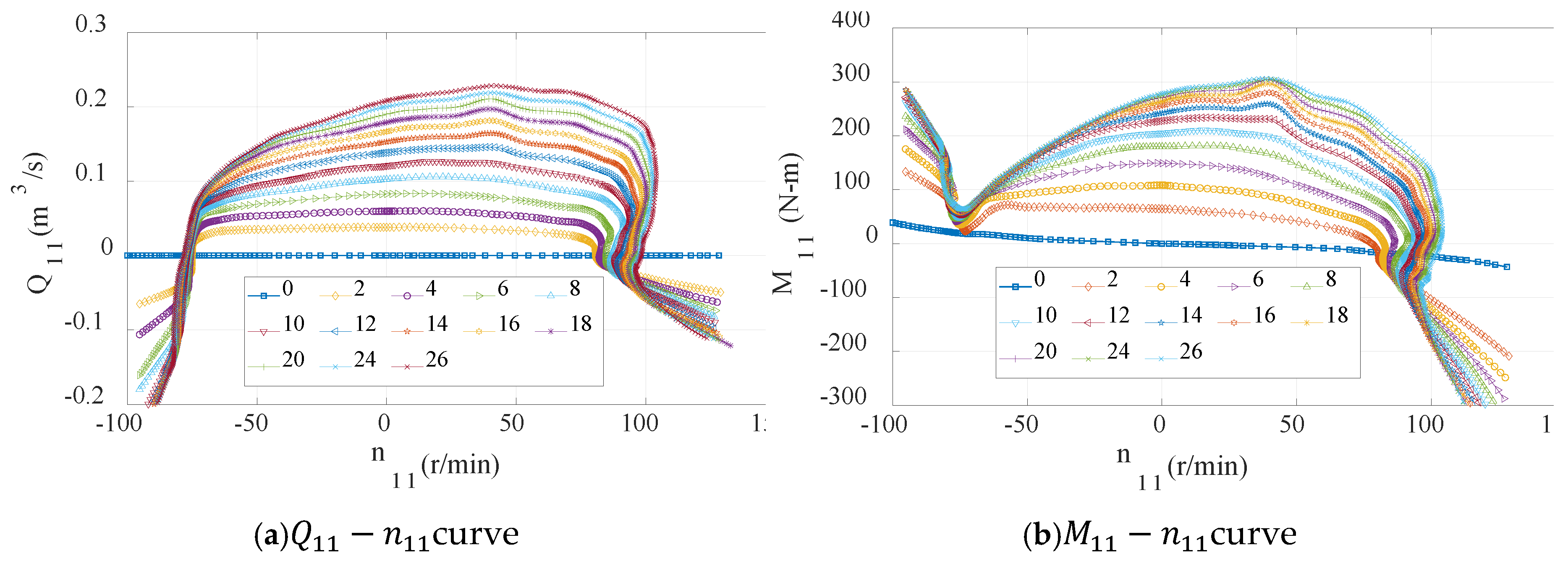
The surge chamber is an important hydraulic facility and mainly plays the role of suppressing water hammer pressure, taking the impedance surge chamber as an example, its equations are composed of momentum, continuity and water level equations.

Momentum equation

$$d{Q}_s/dt=\left(g{A}_s/l\right)\left[H_b-H_s-\left(\mathsf{\xi }/2g{A}_o^2+1/g{A}_s^2\right)\left|Q_s\right|Q_s\right]$$

(10)

Continuity equation

$$Q_t=Q_s+Q_p$$

(11)

Water level equation

$$d{H}_s/dt=Q_s/A_s$$

(12)

where, $Q_s$ is the discharge of surge chamber, m³/s; $A_s$ is the section area of surge chamber, m²; $l$ is the water depth in surge chamber, m; $H_b$ is the water head at the bottom of surge chamber, m; $Q_t$ is the discharge in tunnel, m³/s; $Q_p$ is the discharge of the PT, m³/s; $H_s$ is water level in surge chamber, m; $A_o$is the impedance orifice area of surge chamber, m²; $\mathsf{\xi }$ is the hydraulic loss coefficient of impedance orifice.

Consequently, the boundary of surge chamber can be written:

$$Q_s^i=Q_t^i-Q_p^i$$

(13)

$$H_s^{i+1}=H_s^i+\alpha h\left(Q_s^i/A_s\right)$$

(14)

$$Q_s^{i+1}=Q_s^i+\alpha h\left\{\left(g{A}_s/l\right)\left[H_b^i-H_s^i-\sigma \left|Q_s^i\right|Q_s^i\right]\right\}$$

(15)

where, $\sigma$ is the hydraulic loss coefficient of surge chamber, $\sigma =\left(\mathsf{\xi }/2g{A}_o^2+1/g{A}_s^2\right)$.

2.2.3. Pump-Turbine

In general, the unit parameters of the PT are defined as:

$$n_{11}=n{D}_1/\sqrt{H}$$

(16)

$$Q_{11}=Q/\left(D_1^2\sqrt{H}\right)$$

(17)

$$M_{11}=M/\left(D_1^{3}H\right)$$

(18)

where, $n_{11}$ is the unit speed, rpm; $Q_{11}$is the unit discharge, m³/s; $M_{11}$ is the unit moment, N-m; $n$ is the rotational speed of prototype PT, rpm; $Q$ is the discharge of prototype PT, m³/s; $M$ is the moment of prototype PT, N-m; $H$ is the water head of prototype PT, m; and $D_1$ is the diameter of prototype PT, m.

The complete characteristic curves of the model PT were obtained by model tests in the manufacturing plant, as shown in Figure 2, including $Q_{11}-n_{11}$ and $M_{11}-n_{11}$ curves.

It is evident that the characteristic curves have the inverse “S” feature, resulting in the multiple values in the inverse “S” region during interpolation. Therefore, the Suter transform [21] can convert them into the single-valued curves, and the transform is described as follows:

$$WH\left(x,y\right)=1/\left[{\left(q_1^1+q_{1B}^1\right)}^2+{\left(n_1^1\right)}^2\right]$$

(19)

$$WM\left(x,y\right)=m_1^1$$

(20)

And $\left\{\begin{array}{c}x=atan\left(\left(q_1^1+q_{1B}^1\right)/n_1^1\right)while{n}_{11}\ge 0\\ x=\pi +atan\left(\left(q_1^1+q_{1B}^1\right)/n_1^1\right)whilw{n}_{11}<0\end{array}\right.$where, $q_1^1=Q_{11}/Q_{11r}$, $q_{1B}^1=Q_{11B}/Q_{11r}$, $n_1^1=n_{11}/n_{11r}$, $m_1^1=M_{11}/M_{11r}$, $Q_{11B}$ is generally equal to 0.5$Q_{11r}$ to 1.5$Q_{11r}$, and the subscript 'r' represents the rated value.

Through above transform, $WH\left(x,y\right)-\left(x,y\right)$ and $WM\left(x,y\right)-\left(x,y\right)$ are the single-valued curves. During the calculation of transient process, once $\left(x^i,y^i\right)$ is known, $WH\left(x^i,y^i\right)$ and $WM\left(x^i,y^i\right)$ can be obtained by the interpolation of the single-valued characteristic curves, and $Q_{11}^i$ and $M_{11}^i$ can be reverse calculated by Equations (9) and (10), then the discharge $Q_p^i$ and moment $M_p^i$ of prototype PT can be calculated:

$$Q_p^i=D_1^3{n}^i{Q}_{11}^i/n_{11}^i$$

(21)

$$M_p^i=D_1^5{\left(n^i\right)}^2{M}_{11}^i/{\left(n_{11}^i\right)}^2$$

(22)

where, $Q_p$ is the discharge of prototype PT, m³/s; $M_p$ is the moment of prototype PT, N-m; $D_1$ is the diameter of prototype PT, m; $n$ is the rotational speed of prototype PT, rpm; $Q_{11}$is the unit discharge, m³/s; $M_{11}$ is the unit moment, N-m; $n_{11}$ is the unit speed, rpm.

2.3. Synchronous Generator

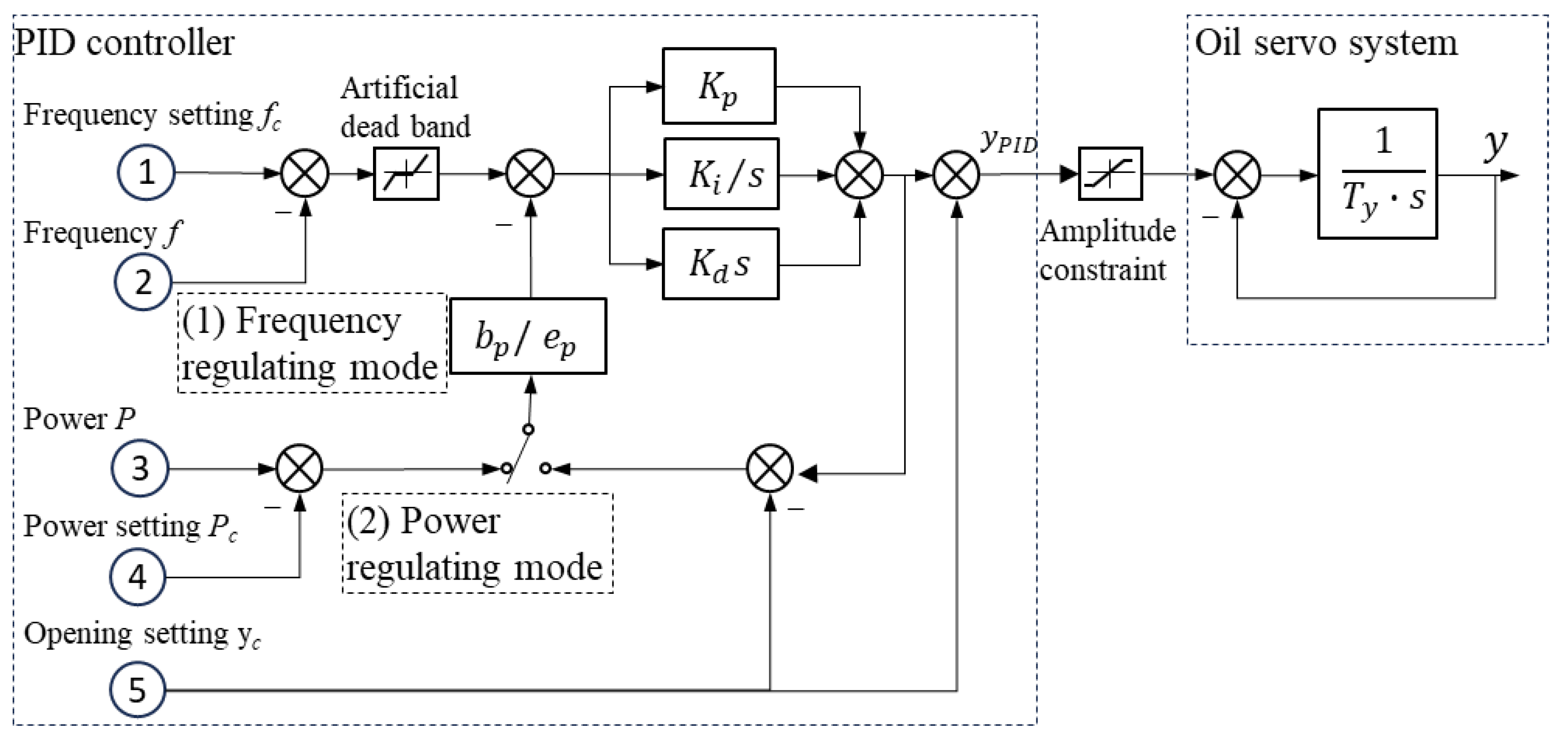
The rotor rotation operation of synchronous generator is described by the following first-order governing equations:

$$dn/dt=9.55\left(M_p-M_g\right)/J$$

(23)

where $n$ is the rotational speed of prototype PT, rpm; $J$ is the inertia, N-m²; $M_p$ the moment is of prototype PT, N-m; $M_g$ is the resistance torque of the rotor, N-m.

Hence, the discrete algorithm for synchronous generator model can be expressed:

$$n^{i+1}=n^i+9.55\alpha h\left(M_p^i-M_g^i\right)/J$$

(24)

2.4. Governor

A microcomputer governor with the parallel PID regulation law is adopted, as shown in Figure 3, which is composed of the PID controller and oil pressure servo system. In the cases of start-up, no-load and isolated grid operation, the frequency regulation mode is preferred. Once the PTU is connected to the power grid, the power regulation mode is prioritized to respond quickly to load change. The main parameters of governor are shown in Table 1.

Under frequency regulation mode, the algorithm of the GVO is derived.

$$y^i=\left[(K_d{s}^2+K_{p}s+K_i)/(b_p{K}_d{s}^2+\left(b_p{K}_p+1\right)+b_p{K}_i)\right]\left(1/(T_{y}s+1)\right)∆f^i$$

(25)

$$∆f^i=f_c-f^i=\left(p/60\right)\left(n_r-n^i\right)$$

(26)

where, $∆f$ is the frequency error of generator, Hz; $f_c$ is the rated frequency of generator, Hz; $n_r$ is the rated rotational speed of generator, rpm; $p$ is the number of pole pairs of the generator.

Similarly, under power regulation mode, the algorithm of the GVO can be written as following:

$$y^i=\left(K_p+K_i/s+K_{d}s/(T_{v}s+1)\right)\left(1/(T_{y}s+1)\right)e_p∆P^i$$

(27)

$$∆P^i=P_c-P_g^i$$

(28)

$$P_g^i=\pi {\mathsf{\eta }}_g{n}^i{M}_p^i/30$$

(29)

where, $∆P$ is the power error of generator, MW; $P_c$ is the power setting of generator, MW; $P_g$ is the power of generator, MW; ${\mathsf{\eta }}_g$ is the efficiency of generator, %.

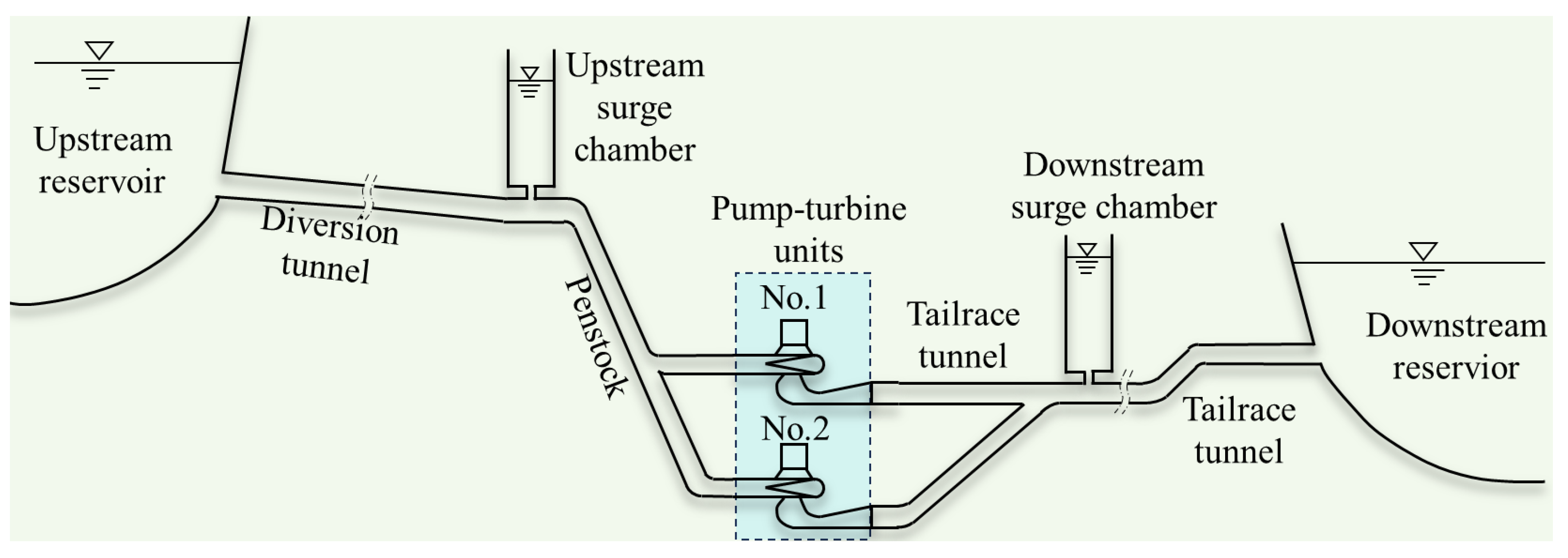
3. Project Overview and Parameters

The PSPS plans to install four Francis PTUs with a single capacity of 350MW, and a total installed capacity of 1400 MW. They undertake the tasks of peak regulation, valley filling, energy storage, frequency regulation, phase regulation, and emergency backup in the power grid. The power station consists of an upstream reservoir, diversion system, underground workshop, switch station, and downstream reservoir. The normal water level of upper reservoir is 1667m, and the regulation capacity is 6.51 million m³. The diversion system adopts the layout of “one diversion tunnel with two PTUs”, which is composed of the inlet/outlet of upstream reservoir, diversion tunnel, upstream surge chamber, penstock, downstream surge chamber, tailrace tunnel, and the inlet/outlet of downstream reservoir. The normal water level of downstream reservoir is 1085m, and the regulation capacity is 7.16 million m³. The layout of one hydraulic unit is shown in Figure 4, and the main parameters of the PTU are shown in Table 2.

Since the diversion tunnel is shared by two PTUs, there is strong hydraulic interference between two PTUs. Therefore, there are seven schemes of peak staggered valley filling to be carried out and optimize the start-up process, and the description of the schemes refers to Table 3.

4. Results & Discussion

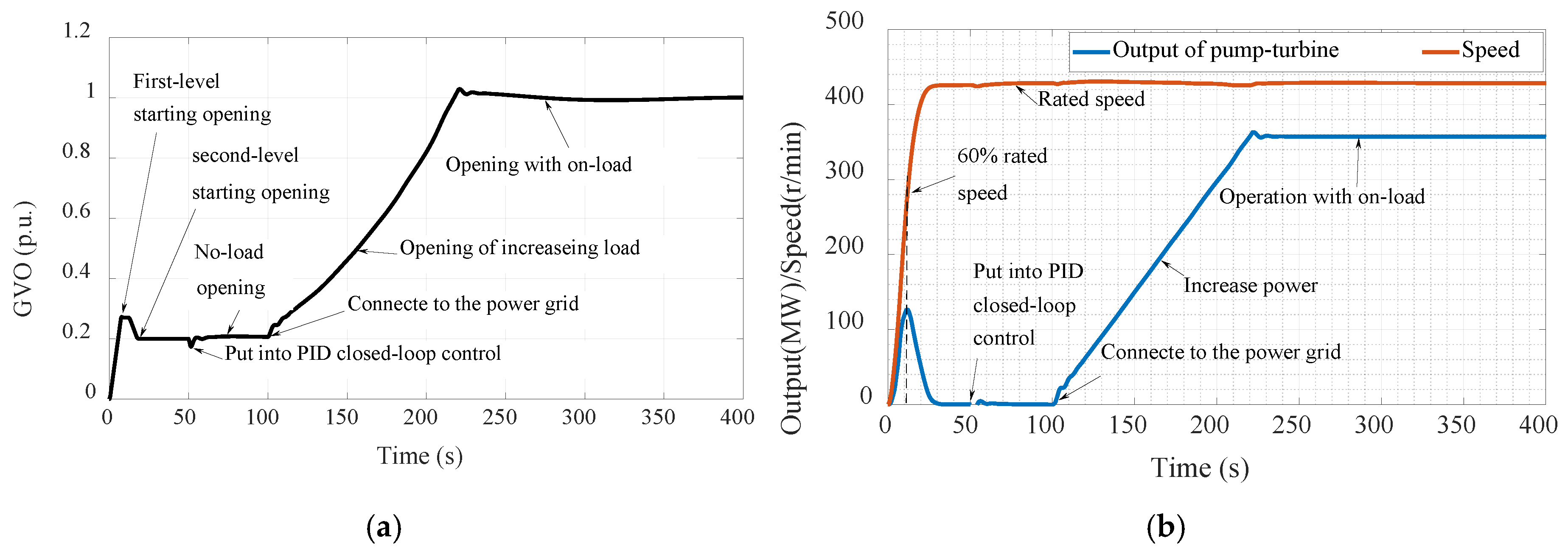
4.1. Transient Process of Start-Up and On-Load

The start-up transient process is shown in Figure 5. Firstly, the guide vane opening (GVO) is set at the first-level starting opening (1.5 to 2.0 times no-load opening) in order to accelerate the starting process of the PTU; When the rotational speed rises to 60% rated speed, the GVO setting is called back to the second-level starting opening (no-load opening) to reduce the acceleration of the PTU; When the rotational speed rises to 95% rated speed, the governor PID control (frequency regulation mode priority) is put into work, and under the control of governor, the PTU will quickly reach the rated speed, and enter no-load operation. Once the rotational speed of the PTU is stable, the generator circuit breaker closes, and the PTU is connected to the power grid, then the PTU runs from no-load to rated load within 2 minutes to complete the on-load process of starting up.

The water level fluctuation in the upstream and downstream surge chambers is shown in Figure 6 and listed in Table 4 during the start-up process. The interval time of start-up between two PTUs is defined as Δt in Figure 6.

When two PTUs are started up at the same time (Δt=0.0s), the water level fluctuation amplitude in surge chamber is large due to the variation of large discharge. It can be seen from Table 4, the water level differences in the upstream and downstream surge chambers reach 9.71m and 1.88m, respectively, which lead to a long fluctuation duration.

The results show that after the PTU No.1 is started up, when the discharge flowing into upstream surge chamber is the largest (scheme 4, Δt=80.0s), then the PTU No.2 is started up, the water level fluctuation in upstream surge chamber is the smallest. Correspondingly, the water level difference in upstream surge chamber is 5.17m, which is only 53.24% of the water level difference when the two PTUs are started up at the same time; The water level difference in downstream surge chamber is 1.37m, which is 72.87% of the water level difference when the two PTUs are started up at the same time. Accordingly, the appropriate start-up interval time is very important to suppress the water level fluctuation of in surge chambers and improve the dynamic characteristics of the PTUs.

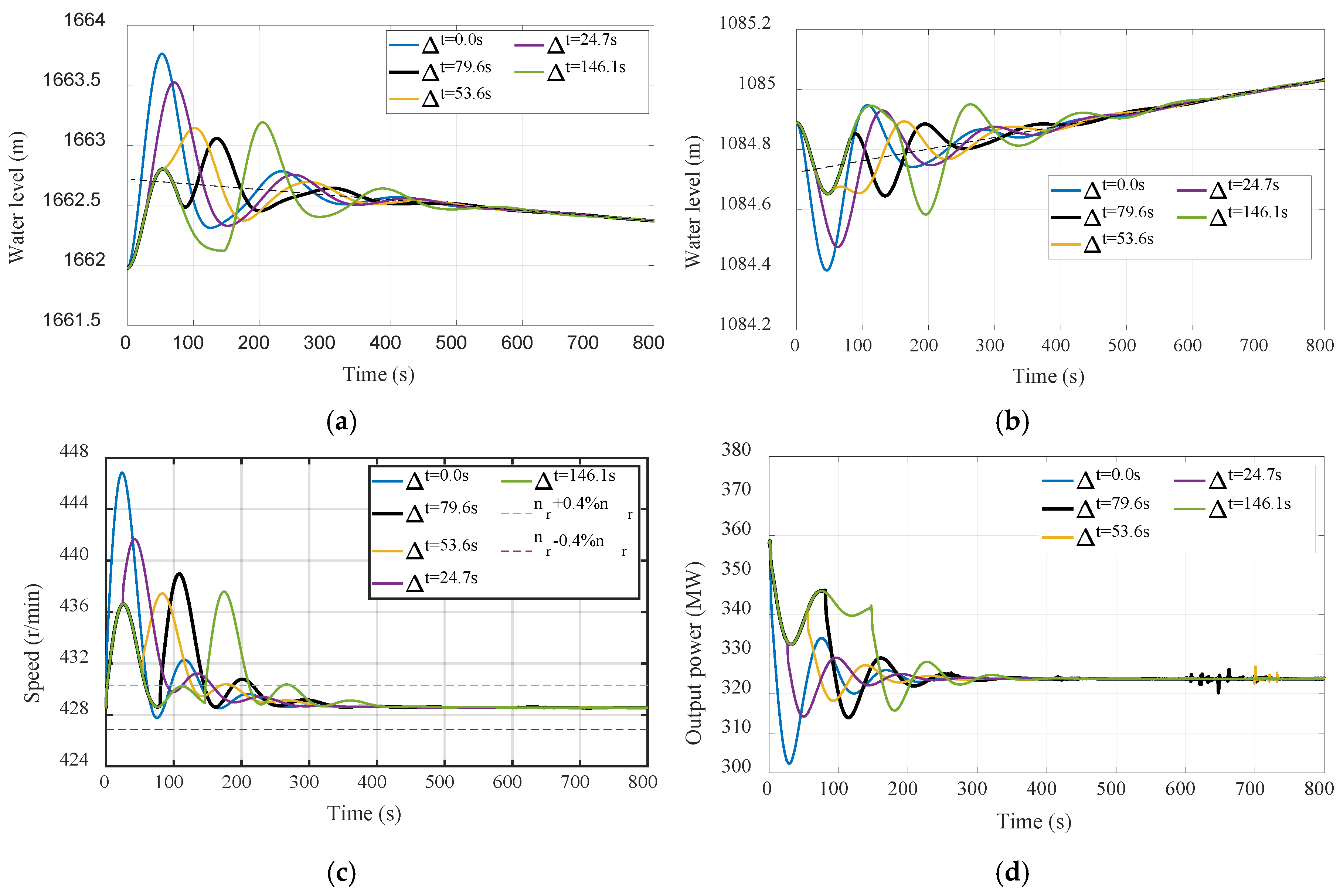
4.2. The Transient Process of Load Regulation Under Power Generation Mode

Taking the rated head, rated power, isolated power gird operation, and 10% load reduction as an example, the results are shown in Figure 7 and Table 5. When the load of two PTUs is reduced at the same time, the water level fluctuation amplitude in upstream/downstream surge chambers is the largest. Similarly, the method of peak staggering and valley filling can be used to reduce the water level fluctuation amplitude in surge chamber and the rotational speed fluctuation amplitude of the PTU to improve the transient characteristics of the PT regulating system. After the load of the PTU No.1 is reduced, when the discharge flowing out the upstream surge chamber is the largest, the load of the PTU No.2 is reduced, that is, the interval time of load reduction between the two PTUs is 79.6s (scheme 2), the water level fluctuation amplitude in upstream and downstream surge chambers is the smallest, and the rotational speed regulation time of the PTU is relatively short.

On the other hand, Figure 7c,d show that after the load of the PTU No.1 is reduced, when the discharge flowing in and out the upstream surge chamber is zero, that is, the load reduction interval time between two PTUs is 53.6s (scheme 3), the rotational speed and power fluctuation amplitude of the PT are the smallest, which is only 48.46% of scheme 1, and the regulation time Tp is the shortest, which is only 126.40s. Consequently, it is difficult to achieve the minimum amplitude of water level fluctuation and rotational speed fluctuation at the same time by using the peak staggering and valley filling, because the water level fluctuation period of surge chamber is not synchronized with the rotational speed fluctuation period of the PTU. Therefore, during the load regulation process, priority should be considered to suppressing rotational speed fluctuation to ensure power quality.

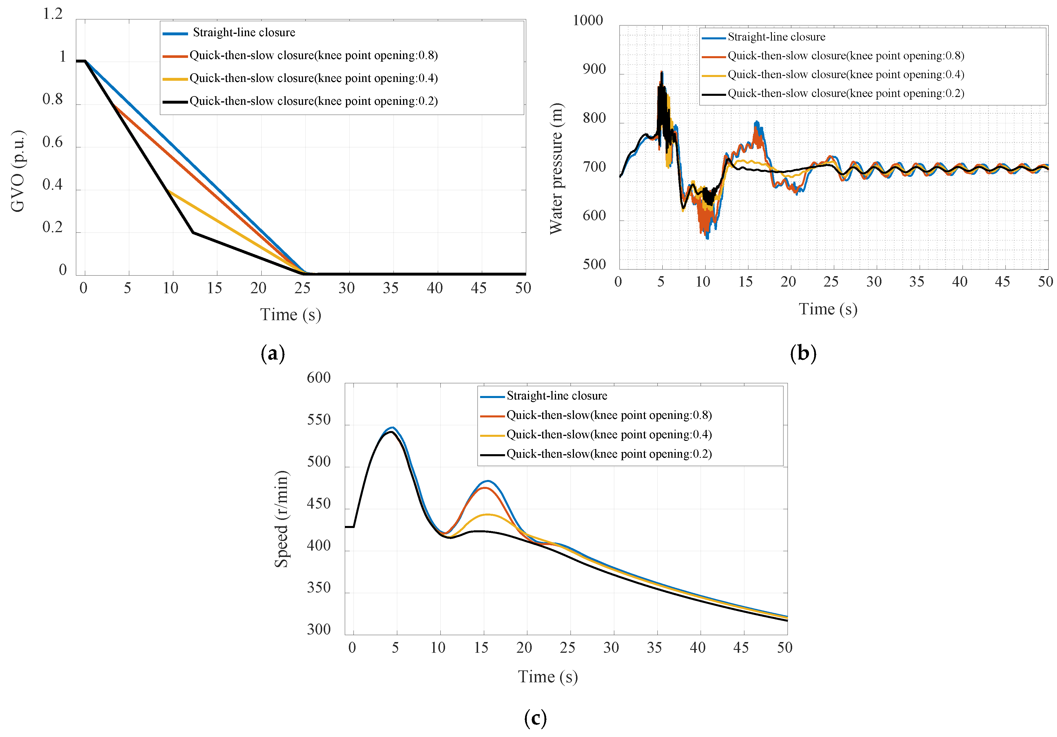
4.3. Transient Process of Load Rejection

Due to the inverse “S” characteristic curve of the PT, a large pulsating pressure is often occurred after load rejecting, resulting in serious vibration of the PTU [22]. In this section, the straight-line closure law and quick-then-slow closure law of the guide vanes are compared, and the knee point opening of the quick-then-slow closure law is optimized. The guide vane closure laws are shown in Figure 8a, and the corresponding knee point openings are listed in Table 6. When the GVO is 100%, the corresponding total closure time is 25.0s. Under the rated operating condition, when the two PTUs reject the full load at the same time, the pressure in the spiral case and the rotational speed of the PTU are shown in Figure 8b,c and Table7.

When the straight-line closure law (scheme 1) is adopted, the maximum water pressure (water hammer pressure + pulsating pressure) in the spiral case is 904.78m, and the PTU stays in the reverse "S" zone for a long time, and the pulsating pressure duration is about 22.0s, as shown in Figure 8b. The maximum rotational speed of the PTU is 547.04 rpm, and there are three rotational speed wave peak values, as shown in Figure 8c. When the quick-then-slow closure law is adopted, with the decrease of knee point opening, the duration of water pressure and pulsation pressure gradually decreases, and the number of rotational speed wave peak and the second peak value also decrease. When the knee point opening is 20.0%, the duration of pulsating pressure is only about 12.0s, and the second wave peak of rotational speed is close to disappearing. Obviously, the quick-then-slow closure law has a significant improvement on the transient process of load rejection.

5. Conclusions

In this paper, the variable time step model of the pump-turbine regulation system of the PSPS with the layout of “one diversion tunnel with two PTUs” is developed, and the typical transient processes of start-up, load regulation and load rejection in the power generation mode are calculated, and the following conclusions are obtained:

1) The appropriate start-up interval time is very important to suppress the water level fluctuation of the surge chambers and improve the transient characteristics of the PTUs. The results show that after one PTU is started up, when the discharge flowing into the upstream surge chamber is the largest, then another PTU is started up, the transient characteristics of the PTUs is the best.

2) The peak staggered valley filling method is difficult to minimize the water level fluctuation amplitude of surge chamber and the rotational speed fluctuation amplitude of the PTU simultaneously, because their fluctuation periods are not consistent. Therefore, during load regulation process, frequency fluctuation should be controlled as a priority to improve the transient characteristics of the PTU.

3) Compared with the traditional characteristic line method, the presented method captures the pulsating pressure well. And the quick-then-slow closure law during load rejection, especially the knee point opening of the guide vanes is within 40%, can significantly improve the characteristics of transient process, and shorten the duration of pulsating pressure.