
Submitted:
16 January 2025
Posted:
20 January 2025
You are already at the latest version
Abstract
Background/Objectives: Manual tuning of exoskeleton control parameters is tedious and often ineffective for adapting to individual users. Human-in-the-loop (HIL) optimization offers an automated approach, but existing methods typically rely on metabolic cost, which requires prolonged data collection times of at least 60 seconds. Surface electromyography (EMG) signals, as an alternative, enable faster optimization with reduced data acquisition times. This study develops a rapid EMG-based HIL Bayesian optimization framework to tune hip exoskeleton controllers for assisting free leg swinging. Methods: Eight participants are asked to perform leg swinging at two frequencies with assistance from a hip exoskeleton. EMG signals from four sensors, representing muscle activity during forward and backward swings, are dynamically processed into cost functions. Bayesian optimization with Gaussian processes tunes four controller parameters using an Expected Improvement acquisition function. Optimization outcomes are validated against no device, zero torque, and general control baselines. Results: Optimization converged within 142 ± 24 seconds, yielding muscle activity reductions of 16.1 compared to no device, 21.7% versus zero torque, and 15.1% versus general control (p < 0.001 for all). EMG-based tuning is faster than metabolic-cost-based methods and perceived as less effortful, with Borg scale reductions of up to 39.5%. Conclusions: EMG-based HIL optimization significantly enhances controller tuning speed and effectiveness, demonstrating its potential for scalable and user-specific exoskeleton applications.
Keywords:
exoskeletons
; human-in-the-loop
; electromyography
; hyperparameter optimization
1. Introduction
Despite several examples of moderate energy reduction improvements in the realm of assistive exoskeletons, most devices still cannot fully account for high inter-subject variability in physiological responses [1,2,3,4,5,6,7]. Slight differences in exoskeleton actuation can significantly affect how users benefit from the assistance. Therefore, more thorough individualized control tuning can achieve better assistance to reduce the effort required to perform certain activities such as walking [8,9,10,12,13,14,15]. The ever-increasing demand for wearable robotics makes manual tuning of control parameters for each individual time-consuming and often strenuous [15,16,17,18]. With human-in-the-loop (HIL) technology, a paradigm that eliminates the need for expert intervention and extensive research hours, optimal parameters are automatically identified and tuned in real-time via physiological signals [8,14,15,19].
While several HIL optimization methods have shown success [2,8,18,19,27], they commonly rely on metabolic cost—a measure with a prolonged acquisition time [22,24,25]. Data measurements for metabolic cost often adapt slowly [12], estimations require substantial historical data [23], and signal readings are influenced by complex neurocognitive factors [24]. Due to these factors, traditional metabolic cost calculations may require 4-6 minutes of data per condition [2,26]. Some alternatives explore accelerating this process by estimating metabolic cost steady state. However, metabolic cost estimations typically demand one to two minutes of data per evaluation [25]. Since thorough optimization requires the evaluation of several conditions, the acquisition time aggregates to a lengthy procedure, allowing the user preference to shift before optimization completion [8,14]. A faster promising alternative is surface electromyography (EMG), a non-invasive measure of muscle activity voltage.
The integration of EMG and exoskeletons is not a novel concept; EMG signal input has been used for modulating control in exoskeletons for several decades [27,28]. While most implementations focus on volitional control of upper body prosthetics and orthotics, some devices employ EMG-control to assist the lower body [27,29]. Studies even demonstrate the successful use of EMG signals to optimally tune walking exoskeleton controllers [8,18]. However, while several studies, including those referenced here and others [8,18], demonstrate the potential of EMG signals as an objective metric in HIL optimization, challenges such as signal noise, poor repeatability, and local metric insights remain underexplored [31,33]. Despite these drawbacks, EMG offers a shorter acquisition time, lower discomfort for subjects, and the ability to reflect reductions in energy economy effectively [32,33,34,35]. Therefore, improving the harnessing of this physiological metric has the potential to significantly reduce the time required for current hardware optimization methods.
In addition to using EMG as the cost function, we employ Bayesian optimization to improve the sample efficiency of our HIL optimization approach. We select Bayesian optimization for its noise tolerance, ability to quickly optimize physiological signals, and documented history of successful outcomes in HIL optimization [19,35,36].
The focus of this work centers on assisting stationary leg-swinging. Leg swinging is a pivotal component of walking and the hip is a natural contender as the joint to target, given its crucial contribution of up to 45% of the mechanical power during the walking gait cycle [1,37]. However, walking is typically analyzed as a whole, focusing on both the stance and swing phases simultaneously, which can mask the specific effects that exoskeleton assistance has on muscle activation during leg swinging alone [1,37]. Therefore, by isolating and optimizing leg-swinging, we aim to develop more targeted and efficient control tuning that can later be integrated with stance phase optimization for full gait cycle assistance.
This work delves into the parameter optimization of an autonomous, self-contained, semi-rigid hip exoskeleton with one degree of freedom (hip extension, hip flexion) to assist leg swinging at two different swing frequencies. The overview of our methods is highlighted by (Figure 1). The novel contributions of this work are the following: 1) We establish a novel EMG-based HIL optimization framework that integrates Bayesian optimization with a dynamic EMG processing pipeline, offering a reliable and efficient solution for tuning assistance controllers across different conditions. 2) We demonstrate that the proposed method significantly reduces tuning time, achieving optimization in as little as 15 seconds per condition, outperforming both metabolic cost-based approaches and prior EMG-based methods. 3) We validate the optimized controllers by demonstrating significant reductions in muscle activity (EMG) compared to baseline conditions, confirming the efficacy of the tuned controllers in improving assistance.
2. Materials and Methods
2.1. Hip Exoskeleton Device
The device used in this study is a custom hip exoskeleton intended to assist hip flexion and extension (Figure 2a). The device is composed of a 24V Brushless DC (BLDC) motor (AK70-10 T motor, 25Nm peak torque, 8Nm nominal torque), attached by a series of straps (shoulder straps, leg straps, belt) and limited rigid components (plastic braces, aluminum links). The actuation is provided in a quasi-direct manner with an open-loop torque controller that allows backdriveability. The angle of the hip is measured by an inertial measurement unit (IMU) (Adafruit BNO055, close-loop triaxial 16-bit gyroscope, 100 Hz reading frequency). The device allows for a maximum range of motion between -30°(extension/posterior) and 90 °(flexion/anterior). The hip exoskeleton also contains elements to prevent injury and discomfort. These features include hard stops at the end of the range of motion to prevent over-extension beyond the comfortable range of motion of the human anatomy, two emergency stop buttons (one to stop the torque and the other to shut down the device), and integrated safety checks in the code to ensure the torque magnitude does not exceed 25 Nm.
The control operates on two levels: high-level control occurs within Python 3.9.2 on a Raspberry Pi 4. This controller replicates torque shapes identified as effective in a prior study [39], employing cubic Bezier curves to define torque magnitude versus angle. These curves, comprising four points in a two-dimensional plane across the swing phase (Figure 2b), require eight inputs: location and magnitude coordinates for each point. The Bezier curves afford flexibility in torque profile shaping without explicit analytic definition.
In this study, the control inputs are further simplified by spacing control points 5° apart and equalizing their magnitudes, reducing the inputs from eight to four. This controller type has shown promising assistance profiles previously [39]. Leg swing control is divided into forward and backward directions, managed separately by a finite state machine (FSM). State transitions are initiated based on changes in angular velocity as detected by the IMU. To preserve natural swing dynamics, the controller synchronizes the torque direction with the velocity direction, ensuring that the assistance contributes positively to the motion.The high-level control signals are updated and sent to the low-level motor controller with a set bandwidth of 100 Hz. The low-level motor control occurs at the motor, where high-level commands are transmitted via the CAN bus protocol to the integrated motor board at a frequency of 1M Hz.
2.2. EMG Data
2.2.1. Sensor Placement and MVC Determination
Surface EMG data was collected using Trigno sensors (Delsys, MA, USA), placed on the rectus femoris (RF) and biceps femoris (BF) of each leg at a sampling frequency of 1778 Hz. Additionally, angle orientation data is collected from the same sensors at 148 Hz. To ensure consistency and comparability, the placement of sensors follow the standardized guidelines provided by the Surface Electromyography for the Non-Invasive Assessment of Muscles project [40].
After sensor placement, the maximum voluntary contraction (MVC) of each targeted muscle is determined by performing maximal muscle contractions against resistance while seated in a stable position to minimize the risk of injury. The RF MVC is measured during a seated knee extension against fixed resistance, and the biceps femoris MVC is assessed during a seated knee flexion. Each MVC trial lasts three seconds and is repeated two times, with rest intervals to prevent fatigue. The highest recorded value from these trials is used for normalization.
2.2.2. Signal Preprocessing
The EMG data from the four sensors is processed in MATLAB using a pipeline optimized for signal-to-noise ratio, as determined in a pilot study. The first step involved bandpass filtering the raw EMG signals between 20 Hz and 450 Hz to eliminate low-frequency noise and high-frequency interference.
Next, an outlier detection algorithm is applied to handle artifacts caused by motion or electrical interference. Extreme values exceeding three standard deviations from the mean are replaced using modified Akima cubic Hermite interpolation [41]. This step improves the reliability of the signal without distorting the physiological envelope, ensuring clean data for subsequent optimization (Figure 3a).
2.2.3. Signal Rectification and Dynamic Smoothing
After filtering and artifact removal, the EMG signals are rectified by taking the absolute value of the signal and subtracting the mean of the non-rectified values to account for any DC offset (Figure 3a). A three-step smoothing process is then applied:
- A moving max filter with a window size of up to 50 data points (less than 0.25% of the total dataset length) is used to highlight signal peaks.
- A discretization filter reduces the resolution of the data using bin sizes between 10 and 30.
- A moving average filter with a window size of up to 400 data points (∼1.6% of the dataset length) smoothes the overall signal (Figure 3b).
These values are selected using an optimization process that maximizes the signal to noise ratio (SNR) of the EMG data. The calculation for SNR is determined by Equation (1).
After this the signals are normalized by dividing each sensor’s output by its corresponding MVC value, allowing the four signals to be combined for further analysis (Figure 3b).
2.2.4. Angle and Velocity Data Integration
The angle data collected from the sensors is linearly interpolated to match the frequency of the EMG data. This interpolated data is differentiated with respect to time to compute velocity. The velocity data is then used to split the EMG signals into forward and backward swing datasets (Figure 3c).
2.2.5. Epoching and Cost Function Calculation
The forward and backward swing datasets are segmented into epochs and averaged to create a single representative signal for each swing phase. This process is repeated for the EMG data collected from the four sensors (RF and BF of both the swing and stance legs) under two different swing frequencies (slow and fast). As a result, eight distinct signals are produced: four sensors × two swing frequencies.
For subsequent analysis, these eight representations are used to calculate two cost functions: one for the forward swing and one for the backward swing. Each cost function is derived by summing the root mean squared (RMS) values of the four EMG signals relevant to that swing phase (Equation (2)).
Here, represents data associated with the forward direction, and represents data associated with the backward direction. The EMG data from the muscle models for the RF and BF of the swing leg, as well as the RF and BF of the stance leg, are represented as , respectively. This process is applied to both slow-swing and fast-swing datasets.
2.2.6. Data Convergence
To ensure the reliability of the EMG data for subsequent analysis, it was essential to determine when the signals reached a steady state. The steady state is defined as the point where the rate of change of the processed EMG signal became negligible, indicating consistent muscle activity over time.
The steady-state condition is analyzed by computing a running average of the EMG signal and monitoring the rate of change over successive time windows. Specifically:
- A running average () at time i is calculated for each sensor using the formula:where represents the signal values at sample j.
- The rate of change () of the running average is computed using a forward difference method:where denotes the running average of the k-th EMG signal at time i.
- These rates of change are aggregated into a single vector g. To analyze the stability of the signal, we segment this vector into windows using a partition method, with a window size w, based on a sampling frequency of 2Hz. This frequency is chosen to balance refined detection (minimal lag) and an ample search window:
- To identify the steady-state point, the rate of change is analyzed within overlapping time windows. Statistical methods, such as a two-sample z-test, are used to compare the mean rates of change between consecutive windows:where and represent the rate of change in the current and previous windows, respectively.
- A p-value of 0.95 is used to confirm no significant difference in the rates of change between consecutive windows. When this condition is met, the signal is considered to have reached a steady state.
The steady-state time is then determined to be the time at which this criterion is satisfied. The steady state is reached under 15 seconds for all participants, ensuring sufficient reliability for subsequent processing.
2.3. Experimental Protocol
A one-day protocol is conducted with eight healthy participants (age: 26.3 ± 3.2 years; weight: 64.6 ± 3.47 kg; height: 165.33 ± 11.13 cm, male: 5, female: 3). Subjects are asked to swing their right leg while their upper torso is supported by a custom rigid structure. The structure restricts the leg swing within a desired angle range (-20° to 30° from the vertical) using bumpers. Two swing frequencies, corresponding with normal walking frequencies [43], are tested (0.67 Hz and 0.83 Hz). These frequencies are encouraged via the use of a metronome which provides the audible cue at which to make contact with each bumper. Participants are instructed to swing their leg at the beat of the metronome such that they make gentle contact with each bumper at each beat (Figure 1). To account for two contacts per swing, the metronome is played at twice the desired swing frequency. A work-to-rest ratio of 1:2 is kept consistent throughout the experiment to reduce the effects of fatigue.
The three-hour experiment consists of four main sections: acclimation, parameter optimization, and validation.
2.3.1. Acclimation
During the acclimation section, subjects are exposed to nine different parameter sets for each swing frequency. The parameter sets are selected using a Latin hypercube sampling (LHS) to provide an even distribution of the parameter space. Each parameter set is supplied for 30-second trials in clusters of three before allowing rest. This results in three slow-frequency clusters and three fast-frequency clusters, each followed by a rest period of 90 seconds. The main focus of this section is to allow participants to learn how to interact with the assistance provided by the device before tuning.
2.3.2. HIL Optimization
We utilize Bayesian optimization as a robust method to identify the optimal set of parameters when the objective function is noisy and expensive to evaluate. This approach involves constructing a probabilistic surrogate model of the objective function which combines prior assumptions about the function with observed data (posterior updates). The surrogate model predicts the objective function’s behavior and incorporates uncertainty, allowing efficient exploration and exploitation of the search space. By leveraging this surrogate model, Bayesian optimization predicts outcomes for different parameter settings and selects the next parameter to evaluate using an acquisition function that balances exploration (trying new settings) and exploitation (utilizing the best-known settings) [44].
In this study, the surrogate model used is a Gaussian Process (GP), a versatile non-parametric approach for modeling distributions over functions. A GP is characterized by a mean function, which represents the expected value of the function, and a covariance function (or kernel), which captures the relationships and dependencies between input points in the parameter space. For simplicity, the prior mean function is assumed to be zero, implying no strong prior belief about the function’s values before observing data. The covariance function used in this study is the Automatic Relevance Determination (ARD) squared exponential kernel, which encodes the similarity between points based on their distance while adjusting for the varying importance of each dimension in the input space. The acquisition function employed is the Expected Improvement (EI) function, which quantifies the potential improvement of the objective function over the best-known value. This function strategically selects the next parameter set to evaluate by maximizing the trade-off between exploration (favoring uncertain areas) and exploitation (favoring areas with high predicted values).
The human-in-the-loop Bayesian optimization procedure involves a maximum of 12 trials for each swing frequency, each lasting 15 seconds. Both swing frequencies are optimized concurrently within the same run, with the slower frequency sampled first, followed by a 10-second rest period, and then the faster frequency.
The initial four trials are initialization trials that sample the parameter space to establish a baseline before the Bayesian optimization begins selecting new parameter sets. The optimization is conducted for up to eight trials, tuning two parameters for both forward and backward swing controllers simultaneously. This results in two controllers being tuned, each with two phases (forward and backward) for both slow and fast frequencies.
Convergence is defined as the same parameter set producing the best-performing controller three times within an allowable variation of ± 10%. If convergence is not achieved within the maximum number of iterations, the experiment continues until all parameter sets converge. The optimal controller is determined as the best-performing parameter set estimated by the Bayesian algorithm.
2.3.3. Validation
Following the identification of the optimal parameter set, its performance is evaluated against three baselines:
- No exoskeleton (NE), where the subject performs free swinging.
- Zero actuation (ZA), where the subject wears the device but it remains unpowered.
- General control (GC), where the subject receives assistance from a predefined intuition controller supplying a magnitude of torque equivalent to the mean of the possible torque values at the beginning of each half swing.
The performance of the optimal and baseline conditions for each swing frequency is tested three times. During each iteration, a performance metric equivalent to the cost function (Equation (2)) is calculated.
Each condition is represented by the mean value of the three observations. The percent change between the optimal mean () and the mean of each baseline () is then calculated. (Equation (7)).
Data collection and processing for each trial follow the same protocol as the tuning trials. Any outliers in the data are identified and replaced with the center value of the data if they deviate by more than three standard deviations from the mean.
Statistical analysis between two conditions is paired. Since the data from most conditions are not normally distributed (Shapiro-Wilk test, p <.05), a non-parametric Wilcoxon test is used to assess the statistical significance of the comparison[45]. The null hypothesis assumes that the average percent change between the optimal and a particular baseline is zero, with a significance level of p <.05.
Additionally, each subject’s perceived effort is rated according to Borg’s scale. While subjective, the Borg Scale has been shown to correlate well with physiological measures such as heart rate, lactate levels, and oxygen consumption. This makes it a reliable complement to the EMG objective measurements in assessing the effectiveness and impact of the exoskeleton [42].
3. Results
This section presents the experimental outcomes, including steady-state signal behavior, optimal controller performance compared to baseline conditions, subjective effort perceptions (via the Borg scale), and optimization process efficiency. Collectively, these results validate the effectiveness of the proposed Bayesian optimization framework in improving EMG-based cost function performance.
To ensure the reliability of the EMG data, steady-state behavior was analyzed. Figure 4 illustrates the steady-state time average for each subject, demonstrating that the rate of change of a running average of the summed EMG data consistently converges within 15 seconds across all trials. This result confirms the stability of the EMG signal during the experimental conditions.
The optimal controller (OP) outperformed all baseline conditions on average (Figure 5). For the slow swing, OP reduced muscle activity by 15.2% (p < 1e-7) compared to the no device condition and by 19.7% (p < 1e-4) compared to the zero torque condition. Additionally, the OP reduced muscle activity by 14.5% (p < 1e-4) compared to the general controller. For the fast swing, OP significantly reduced muscle activity compared to the no device and zero torque conditions by 17.0% (p < 1e-4) and 23.6% (p < 1e-4), respectively, and by 15.6% (p = 0.0015) compared to the fast swing general controller. The optimal controller profiles for all subjects are shown in Figure 6.
In terms of Borg scale values, the optimal controller is perceived to lower effort compared to most baselines. The percent change in mean Borg values between the optimal and each baseline condition is shown in Table 1, calculated using Equation (7).
The Bayesian optimization framework identified a preferred parameter set within an average of 9.5 trials (SD = 1.87). Early stop conditions were met for seven of the eight subjects, confirming the efficiency of the optimization process. For the remaining subject, all but one parameter (Lb) converged, suggesting a strong but incomplete preference by the acquisition function. Figure 7 illustrates optimization landscapes for a sample subject, highlighting the parameter tuning process.
4. Discussion
The optimization process demonstrates a strong ability to tune quickly and effectively, resulting in a significant reduction of muscle activity compared to all baselines. This outcome establishes the importance of tuning, as the optimal controller outperformed arbitrary assistance. The reduction in muscle activity is very likely attributed to the proper timing provided by the controller, which reduces the load on these muscles during critical phases of the leg swing. By delivering targeted assistance, the controller minimizes the energy required for muscle contraction, improving efficiency and reducing fatigue. These results highlight the necessity of fine-tuning controllers for individual users to achieve maximal benefit, especially in tasks involving repetitive motion.
The use of EMG data for tuning further validates its role as an effective and rapid alternative to metabolic cost, particularly given the challenges of metabolic measurements in real-time applications. The study’s ability to achieve tuning in as little as 15 seconds, compared to 60 seconds with traditional metabolic cost-based methods, represents a significant advancement in human-in-the-loop optimization [19]. The reduced tuning time is particularly important in clinical or real-world settings, where prolonged optimization sessions can lead to user discomfort or fatigue.
In comparison with prior EMG HIL optimization studies [46], the consistent controller performance achieved in our study, alongside the shorter tuning duration, further establishes the practicality and scalability of EMG-based optimization. While EMG data provides valuable insights into muscle activation, it may not fully capture the complexity of the energy demands during dynamic tasks like walking or running. Future studies could expand on this by integrating other physiological metrics, such as joint torque or oxygen consumption, to provide a more comprehensive understanding of exoskeleton performance across various activities.
The Borg scale results add another layer of validation to the optimization process by reflecting subjective user experience. The noticeable reduction in perceived effort (Table 1) show that the assistance from the optimal controller provided a noticeable aid while swinging aligns with the objective EMG data. This reinforces the conclusion that the optimized controller provides effective assistance. The significant decrease in perceived effort compared to baseline conditions suggests that users benefit not only physiologically but also experientially from the tuned exoskeleton assistance. These results emphasize the importance of optimizing assistive devices for both performance and comfort, as user satisfaction plays a crucial role in the long-term adoption of wearable technology.
Despite the promising results, limitations should be noted. The reliance on EMG as the sole physiological metric introduces potential variability due to factors such as signal noise and electrode placement. Although the data processing methods effectively mitigate some of these issues, the inherent noisiness of EMG signals suggests that future work should incorporate additional validation metrics to cross-check the findings. Also, investigating the long-term effectiveness of the optimal controller was not addressed in this study. While this study focuses on stationary leg swinging, more dynamic activities such as walking, running, or squatting should be explored to fully understand the exoskeleton’s capabilities in more demanding real-world applications. Investigating how these findings translate to full movement cycle optimization would be an important step toward developing more comprehensive assistive devices. Moreover, the size of the subject pool restricts the generalizability of the results, as individual variations in muscle response and gait patterns could influence the outcomes. A larger, more diverse sample size would allow for more robust conclusions and better correlation analysis.
5. Conclusion
The importance of this study lies in its ability to achieve fast and effective controller tuning and improved EMG processing for optimization. The findings indicate that EMG optimization is not only quick and effective but also worthy of further investigation. The study advances our understanding of rapid EMG optimization, offering promising potential for future research and practical applications in the development of exoskeleton controllers.
Author Contributions
Conceptualization, Echeveste and Bhounsule; methodology, Echeveste; software, Echeveste; validation, Echeveste; formal analysis, Echeveste; investigation, Echeveste; resources, Bhounsule; data curation, Echeveste; writing—original draft preparation, Echeveste; writing—review and editing, Bhounsule; visualization, Echeveste; supervision, Bhounsule; project administration, Bhounsule; funding acquisition, Bhounsule. All authors have read and agreed to the published version of the manuscript.
Funding
This research received no external funding.
Institutional Review Board Statement
The study was conducted in accordance with the Declaration of Helsinki, and approved by the Institutional Review Board of University of Illinois at Chicago Institutional (STUDY 1022-2022).
Informed Consent Statement
Informed consent was obtained from all subjects involved in the study.
Data Availability Statement
Data is unavailable due to privacy or ethical restrictions.
Acknowledgments
The authors would like to thank Subramanian Ramasamy, and ChunMing Yang for volunteering as resident subjects for fine-tuning of the methods. The authors would also like to extend gratitude towards Myunghee Kim and members of the Rehabilitation Robotics Laboratory at the University of Illinois at Chicago for their continued support and assistance.
Conflicts of Interest
The authors declare no conflicts of interest.
Abbreviations
The following abbreviations are used in this manuscript:
| EMG | Electromyography |
| HIL | Human-in-the-loop |
| MVC | Maximum Voluntary Contraction |
| FSM | Finite State Machine |
| RF | Rectus Femoris |
| BF | Bicep Femoris |
References
- Chen, B.; Zi, B.; Qin, L.; Pan, Q. State-of-the-art research in robotic hip exoskeletons: A general review. Journal of Orthopaedic Translation 2020, 20, 4–13. [Google Scholar] [CrossRef] [PubMed]
- Han, H.; Wang, W.; Zhang, F.; Li, X.; Chen, J.; Han, J.; Zhang, J. Selection of muscle-activity-based cost function in human-in-the-loop optimization of multi-gait ankle exoskeleton assistance. IEEE Transactions on Neural Systems and Rehabilitation Engineering 2021, 29, 944–952. [Google Scholar] [CrossRef] [PubMed]
- Martini, E.; Sanz-Morère, C.B.; Livolsi, C.; Pergolini, A.; Arnetoli, G.; Doronzio, S.; Giffone, A.; Conti, R.; Giovacchini, F.; Friðriksson, Þ.; et al. Lower-limb amputees can reduce the energy cost of walking when assisted by an Active Pelvis Orthosis. Proceedings of the 2020 IEEE RAS/EMBS International Conference for Biomedical Robotics and Biomechatronics (BioRob) 2020, 809–815. [CrossRef]
- Malcolm, P.; Derave, W.; Galle, S.; De Clercq, D. A simple exoskeleton that assists plantarflexion can reduce the metabolic cost of human walking. PLOS ONE 2013, 8, e56137. [Google Scholar] [CrossRef]
- Mooney, L.M.; Rouse, E.J.; Herr, H.M. Autonomous exoskeleton reduces metabolic cost of human walking during load carriage. Journal of NeuroEngineering and Rehabilitation 2014, 11, 80. [Google Scholar] [CrossRef]
- Collins, S.H.; Wiggin, M.B.; Sawicki, G.S. Reducing the energy cost of human walking using an unpowered exoskeleton. Nature 2015, 522, 212–215. [Google Scholar] [CrossRef] [PubMed]
- Koller, J.R.; Jacobs, D.A.; Ferris, D.P.; Remy, C.D. Learning to walk with an adaptive gain proportional myoelectric controller for a robotic ankle exoskeleton. Journal of NeuroEngineering and Rehabilitation 2015, 12, 97. [Google Scholar] [CrossRef]
- Zhang, J.; Fiers, P.; Witte, K. A.; Jackson, R. W.; Poggensee, K. L.; Atkeson, C. G.; Collins, S. H. Human-in-the-loop optimization of exoskeleton assistance during walking. Science 2017, 356, 1280–1284. [Google Scholar] [CrossRef] [PubMed]
- Zelik, K. E.; Collins, S. H.; Adamczyk, P. G.; Segal, A. D.; Klute, G. K.; Morgenroth, D. C.; Hahn, M. E.; Orendurff, M. S.; Czerniecki, J. M.; Kuo, A. D. Systematic variation of prosthetic foot spring affects center-of-mass mechanics and metabolic cost during walking. IEEE Trans. Neural Syst. Rehabil. Eng. 2011, 19, 411–419. [Google Scholar] [CrossRef]
- Jackson, R. W.; Collins, S. H. An experimental comparison of the relative benefits of work and torque assistance in ankle exoskeletons. J. Appl. Physiol. 2015, 119, 541–557. [Google Scholar] [CrossRef] [PubMed]
- Quesada, R. E.; Caputo, J. M.; Collins, S. H. Increasing ankle push-off work with a powered prosthesis does not necessarily reduce metabolic rate for transtibial amputees. J. Biomech. 2016, 49, 3452–3459. [Google Scholar] [CrossRef] [PubMed]
- Handford, M. L.; Srinivasan, M. Robotic lower limb prosthesis design through simultaneous computer optimizations of human and prosthesis costs. Sci. Rep. 2016, 6, 19983. [Google Scholar] [CrossRef] [PubMed]
- Farris, D. J.; Robertson, B. D.; Sawicki, G. S. Elastic ankle exoskeletons reduce soleus muscle force but not work in human hopping. J. Appl. Physiol. 2013, 115, 579–585. [Google Scholar] [CrossRef]
- Ferris, D. P.; Sawicki, G. S.; Daley, M. A. A physiologist’s perspective on robotic exoskeletons for human locomotion. Int. J. Humanoid Robot. 2007, 4, 507–528. [Google Scholar] [CrossRef]
- Quesada, R. E.; Caputo, J. M.; Collins, S. H. Increasing ankle push-off work with a powered prosthesis does not necessarily reduce metabolic rate for transtibial amputees. Journal of Biomechanics 2016, 49, 3452–3459. [Google Scholar] [CrossRef]
- Huang, D.; Allen, T. T.; Notz, W. I.; Zeng, N. Global Optimization of Stochastic Black-Box Systems via Sequential Kriging Meta-Models. Journal of Global Optimization 2006, 34, 441–466. [Google Scholar] [CrossRef]
- Lorenz, R.; Monti, R. P.; Violante, I. R.; Anagnostopoulos, C.; Faisal, A. A.; Montana, G.; Leech, R. The Automatic Neuroscientist: A framework for optimizing experimental design with closed-loop real-time fMRI. NeuroImage 2016, 129, 320–334. [Google Scholar] [CrossRef] [PubMed]
- Ren, P.; Wang, W.; Jing, Z.; Chen, J.; Zhang, J. Improving the Time Efficiency of sEMG-based Human-in-the-Loop Optimization. In Proceedings of the 2019 Chinese Control Conference (CCC); 2019; pp. 4626–4631. [Google Scholar] [CrossRef]
- Kim, M.; Ding, Y.; Malcolm, P.; Speeckaert, J.; Siviy, C. J.; Walsh, C. J.; Kuindersma, S. Human-in-the-loop Bayesian optimization of wearable device parameters. PLOS ONE 2017, 12, e0184054. [Google Scholar] [CrossRef] [PubMed]
- Gordon, D. F. N.; McGreavy, C.; Christou, A.; Vijayakumar, S. Human-in-the-loop optimization of exoskeleton assistance via online simulation of metabolic cost. IEEE Transactions on Robotics 2022, 38, 1410–1429. [Google Scholar] [CrossRef]
- Makin, T. R.; de Vignemont, F.; Faisal, A. A. Neurocognitive barriers to the embodiment of technology. Nature Biomedical Engineering 2017, 1, 0014. [Google Scholar] [CrossRef]
- Gordon, K. E.; Ferris, D. P. Learning to walk with a robotic ankle exoskeleton. Journal of Biomechanics 2007, 40, 2636–2644. [Google Scholar] [CrossRef]
- Selinger, J. C.; O’Connor, S. M.; Wong, J. D.; Donelan, J. M. Humans Can Continuously Optimize Energetic Cost during Walking. Current Biology 2015, 25, 2452–2456. [Google Scholar] [CrossRef] [PubMed]
- Makin, T. R.; de Vignemont, F. Neurocognitive Barriers to the Embodiment of Technology. Nature Biomedical Engineering 2017, 1, 0014. [Google Scholar] [CrossRef]
- Selinger, J. C.; Donelan, J. M. Estimating instantaneous energetic cost during non-steady-state gait. Journal of Applied Physiology 2014, 117, 1406–1415. [Google Scholar] [CrossRef]
- Gordon, D. F. N.; McGreavy, C.; Christou, A.; Vijayakumar, S. Human-in-the-Loop Optimization of Exoskeleton Assistance via Online Simulation of Metabolic Cost. IEEE Transactions on Robotics 2022, 38, 1410–1429. [Google Scholar] [CrossRef]
- Gordon, K. E.; Ferris, D. P. Learning to walk with a robotic ankle exoskeleton. Journal of Biomechanics 2007, 40, 2636–2644. [Google Scholar] [CrossRef] [PubMed]
- Rosen, J.; Brand, M.; Fuchs, M. B.; Arcan, M. A myosignal-based powered exoskeleton system. IEEE Transactions on Systems, Man, and Cybernetics - Part A: Systems and Humans 2001, 31, 210–222. [Google Scholar] [CrossRef]
- Cimolato, A.; Driessen, J.J.M.; Mattos, L.S.; De Momi, E.; Laffranchi, M.; De Michieli, L. EMG-driven control in lower limb prostheses: a topic-based systematic review. Journal of NeuroEngineering and Rehabilitation 2022, 19, 43. [Google Scholar] [CrossRef] [PubMed]
- Huang, H.; Zhang, F.; Hargrove, L.J.; Dou, Z.; Rogers, D.R.; Englehart, K.B. Continuous locomotion-mode identification for prosthetic legs based on neuromuscular-mechanical fusion. IEEE Transactions on Biomedical Engineering 2011, 58, 2867–2875. [Google Scholar] [CrossRef]
- Aguirre-Ollinger, G. Learning muscle activation patterns via nonlinear oscillators: Application to lower-limb assistance. In Proceedings of the 2013 IEEE/RSJ International Conference on Intelligent Robots and Systems; 2013; pp. 1182–1189. [Google Scholar] [CrossRef]
- Winter, D.A.; Yack, H.J. EMG profiles during normal human walking: stride-to-stride and inter-subject variability. Electroencephalography and Clinical Neurophysiology 1987, 67, 402–411. [Google Scholar] [CrossRef]
- Huang, H.; Zhang, F.; Hargrove, L.J.; Dou, Z.; Rogers, D.R.; Englehart, K.B. Continuous locomotion-mode identification for prosthetic legs based on neuromuscular-mechanical fusion. IEEE Transactions on Biomedical Engineering 2011, 58, 2867–2875. [Google Scholar] [CrossRef] [PubMed]
- Fleischer, C.; Reinicke, C.; Hommel, G. Predicting the intended motion with EMG signals for an exoskeleton orthosis controller. In Proceedings of the 2005 IEEE/RSJ International Conference on Intelligent Robots and Systems; 2005; pp. 2029–2034. [Google Scholar] [CrossRef]
- Gordon, D.F.N.; Matsubara, T.; Noda, T.; Teramae, T.; Morimoto, J.; Vijayakumar, S. Bayesian optimization of exoskeleton design parameters. In Proceedings of the 2018 7th IEEE International Conference on Biomedical Robotics and Biomechatronics (Biorob); 2018; pp. 653–658. [Google Scholar] [CrossRef]
- Brochu, E.; Cora, V.M.; Freitas, N. de. A Tutorial on Bayesian Optimization of Expensive Cost Functions, with Application to Active User Modeling and Hierarchical Reinforcement Learning. CoRR 2010, abs/1012.2599. http://arxiv.org/abs/1012.2599.
- Yandell, M.B.; Quinlivan, B.T.; Popov, D.; Walsh, C.; Zelik, K.E. Physical interface dynamics alter how robotic exosuits augment human movement: Implications for optimizing wearable assistive devices. Journal of NeuroEngineering and Rehabilitation 2017, 14, 40. [Google Scholar] [CrossRef]
- Yang, C.; Yu, L.; Xu, L.; Yan, Z.; Hu, D.; Zhang, S.; Yang, W. Current developments of robotic hip exoskeleton toward sensing, decision, and actuation: A review. Wearable Technologies 2022, 3, e15. [Google Scholar] [CrossRef] [PubMed]
- Echeveste, S.; Hernandez Hinojosa, E. Optimal Swing Assistance Using a Hip Exoskeleton: Comparing Simulations With Hardware Implementation. In Volume 8: 47th Mechanisms and Robotics Conference (MR), Proceedings of the International Design Engineering Technical Conferences and Computers and Information in Engineering Conference, 2023; V008T08A074. [CrossRef]
- SENIAM, Surface EMG for Non-Invasive Assessment of Muscles. Available online: http://seniam.org/sensor_location.htm (accessed on 13 January 2025).
- Akima, H. (1970). A New Method of Interpolation and Smooth Curve Fitting Based on Local Procedures. Journal of the Association for Computing Machinery 17, 4, 589–602. [CrossRef]
- Miller, L. E.; Zimmermann, A. K.; Herbert, W. G. Clinical effectiveness and safety of powered exoskeleton-assisted walking in patients with spinal cord injury: systematic review with meta-analysis. Medical Devices: Evidence and Research 2016, 455–466. [CrossRef]
- Straczkiewicz, M.; Huang, E. J.; Onnela, J.-P. Physical interface dynamics alter how robotic exosuits augment human movement: implications for optimizing wearable assistive devices. npj Digital Medicine 2023, 6, 29. [CrossRef]
- Brochu, E.; Cora, V. M.; Freitas, N. de. A tutorial on Bayesian optimization of expensive cost functions, with application to active user modeling and hierarchical reinforcement learning. CoRR 2010, arXiv:1012.2599. Available online: http://arxiv.org/abs/1012.2599. [Google Scholar]
- Mishra, P.; Pandey, C.M.; Singh, U.; Gupta, A.; Sahu, C.; Keshri, A. Descriptive statistics and normality tests for statistical data. Annals of Cardiac Anaesthesia 2019, 22, 67–72. [Google Scholar]
- Ma, L.; Ba, X.; Xu, F.; Leng, Y.; Fu, C. EMG-based Human-in-the-loop Optimization of Ankle Plantar-flexion Assistance with a Soft Exoskeleton. In Proceedings of the 2022 International Conference on Advanced Robotics and Mechatronics (ICARM); 2022; pp. 453–458. [Google Scholar] [CrossRef]
Figure 1.
An illustration of the experimental setup for leg swinging, highlighting the exoskeleton device, sensors, and support structure on the left. This also outlines the EMG data processing pipeline, showcasing the four signals used on the top section. Additionally, the optimization process is depicted, detailing how Bayesian optimization tunes four controller parameters based on two cost functions. The bottom aspect of the figure presents the controller’s parameterization and its influence on the torque profile.
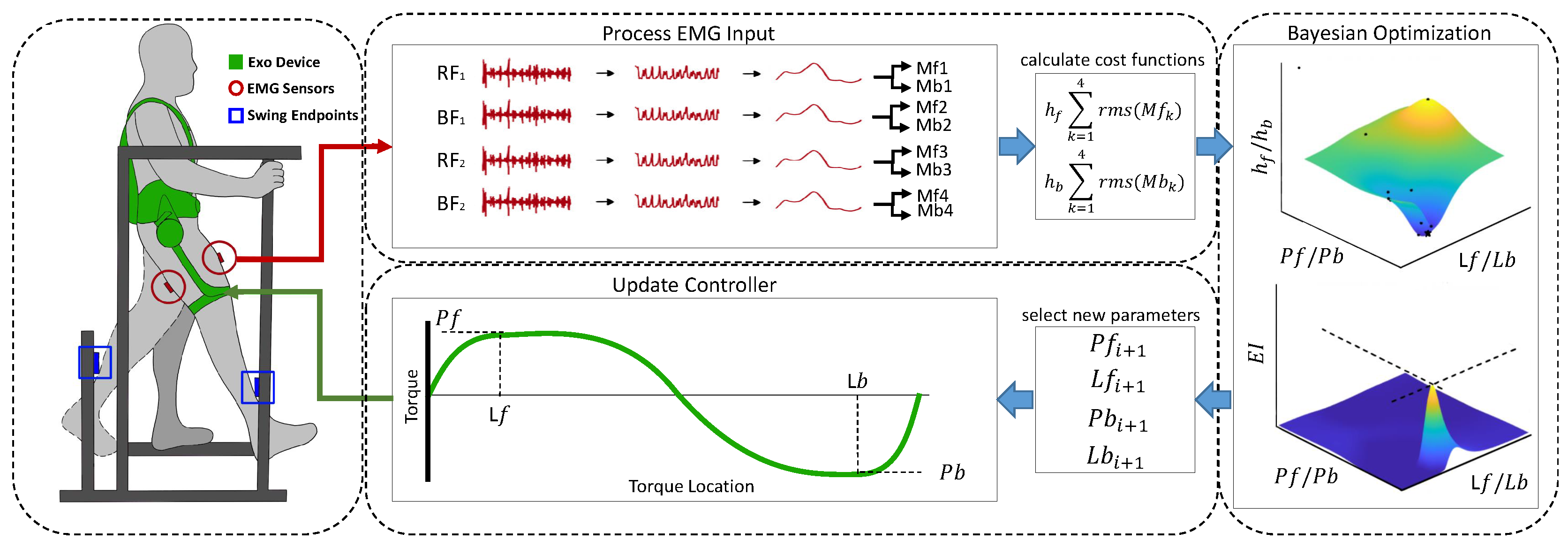
Figure 2.
(a) An illustration of the exoskeleton device detailing all the main components. (b) An overview of the controller constructs a relationship between torque and angle using segmented Bezier curves. The location of the four control points. Control points and are dependent on and while and are dependent on and . The torque functions for forward and backward actuation are represented as and respectively.
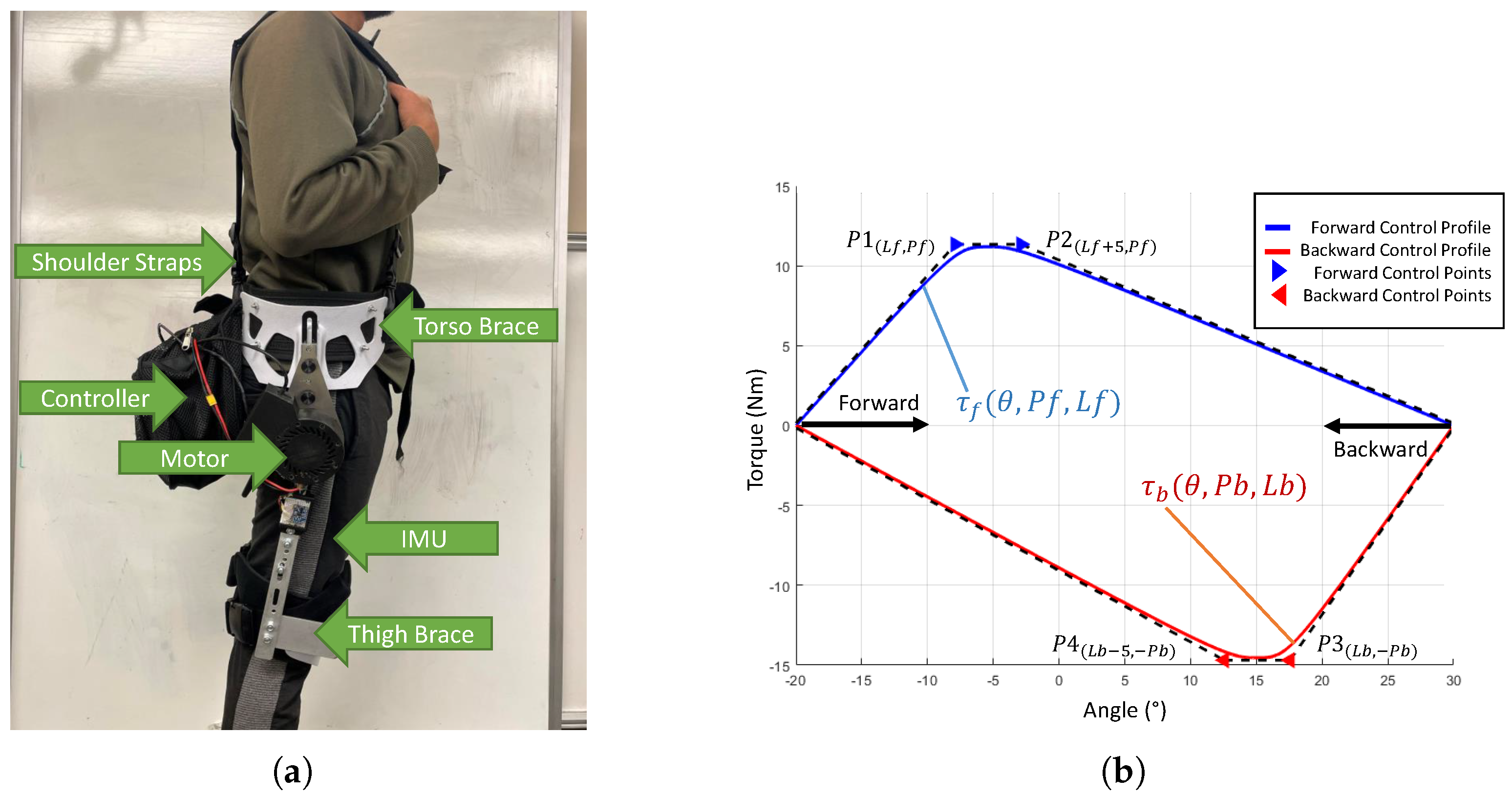
Figure 3.
The visual process in three steps: (a) Signal processing steps including a bandpass filter with a high pass of 20Hz and a low pass of 450Hz plus an outlier replacement of extreme values beyond 3 standard deviations using a modified Akima cubic Hermite interpolation; and rectification by taking the absolute value and subtracting the mean value of the previous signal. (b) Signal processing steps including a moving max and discretization filter to outline the shape of the signal; and a moving average filter to smooth noise followed by normalization against the MVC value for each sensor. (c) Signal processing steps including partitioning the data into separate swings; and a data aggregation process using an averaged representation of the epochs to produce a single output representation.
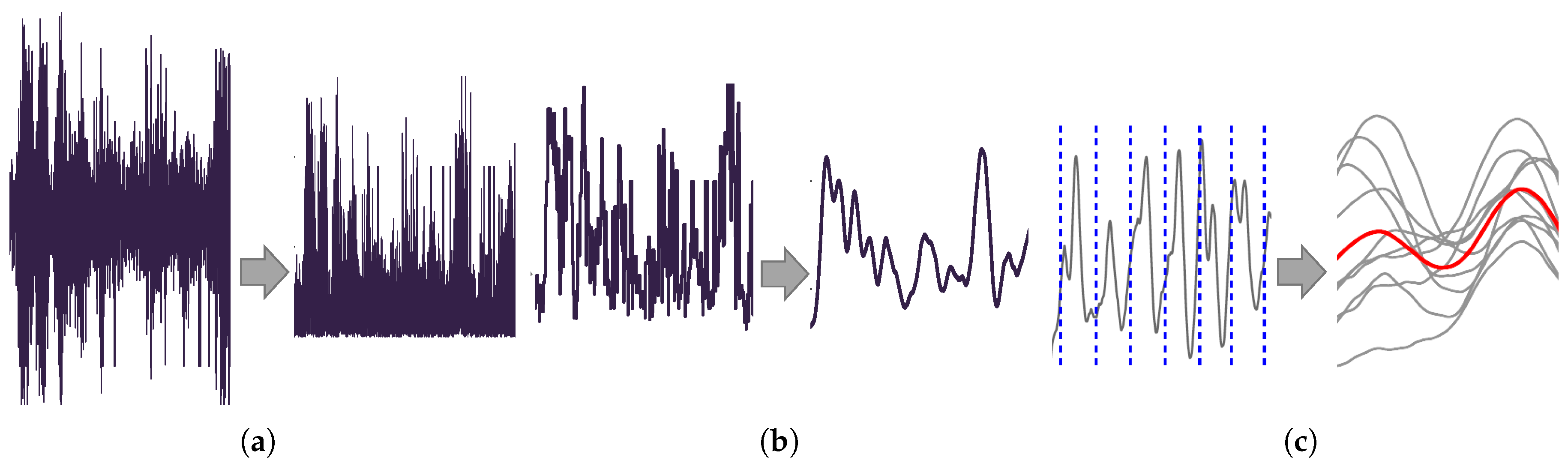
Figure 4.
The convergence data for each subject is represented as a bold average line with dotted lines showing the standard deviation. The variable g represents the sum of the derivative of the running average for the four sensors across all trials of a subject. The star indicates the time when a steady state is reached on average.
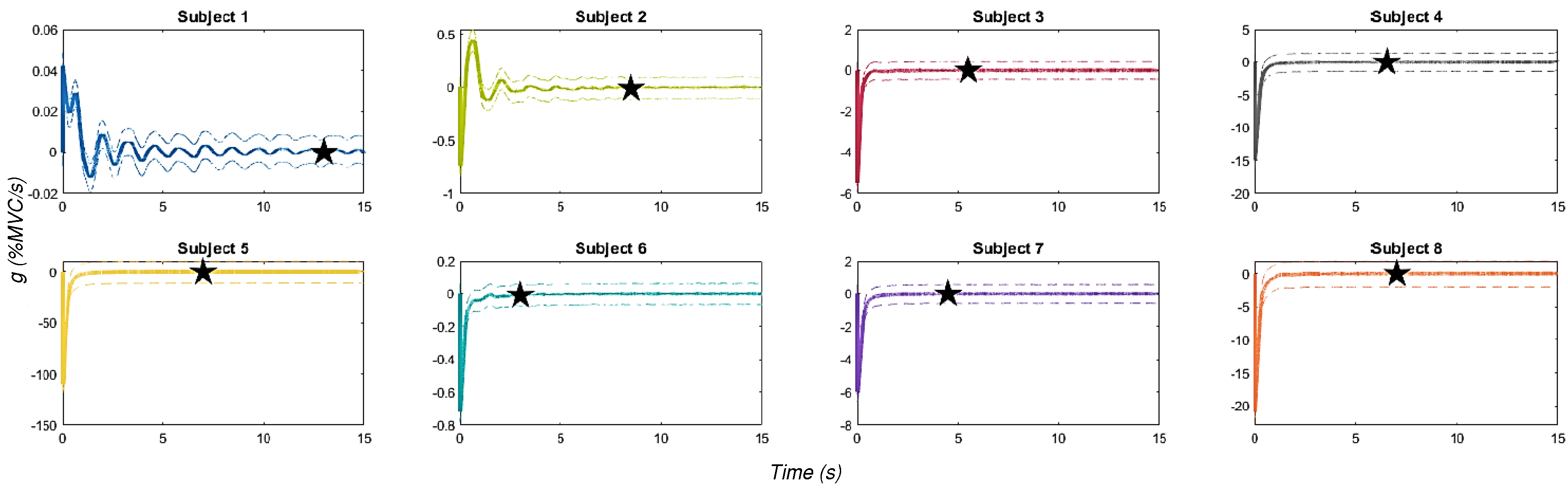
Figure 5.
Condition comparison results from the validation phase. The condition averages of the EMG performance metric are represented by the bar graph. The standard deviation is shown by whiskers. Percent changes between tests with three baseline conditions and tests with optimal control are shown above the horizontal brackets.
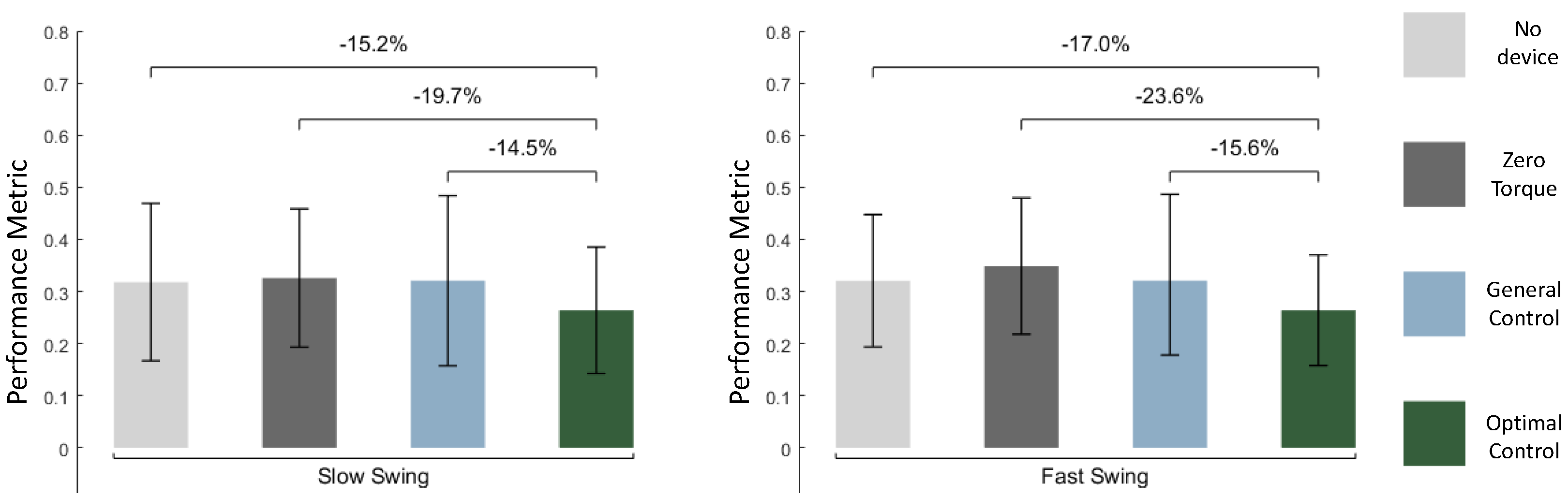
Figure 6.
This figure presents a comprehensive view of the swing controller concerning both controller parameters and torque profiles. The plots on the left display the spatial distribution of controller parameters during the slow swing and fast swing. The x-axis represents the location, and the y-axis denotes the magnitude. The two plots on the right showcase the torque profile for the slow and fast swing, with the x-axis indicating the swing phase as a percentage, and the y-axis representing the weight-normalized torque.
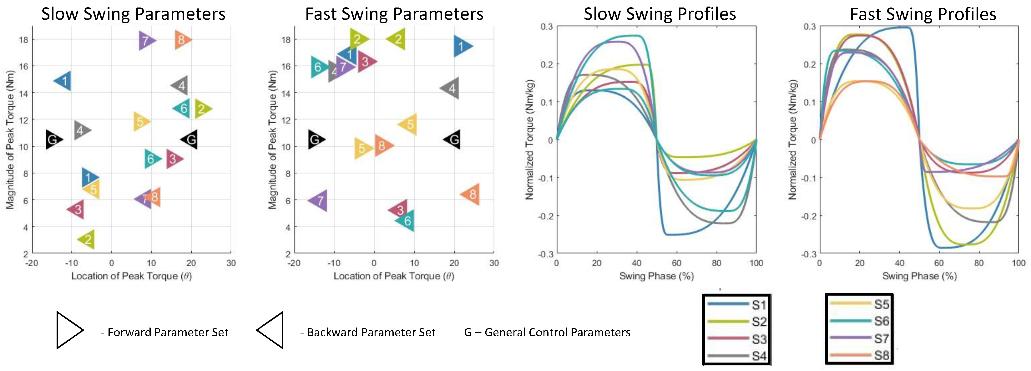
Figure 7.
Three samples of the surrogate and acquisition function optimization landscapes from Bayesian optimization. The h variable represents the cost function, P and L are the two parameters tuned, and EI is the expected improvement for each parameter set. Lower values are favorable for the Gaussian process model, and higher values are favorable for the expected improvement function.
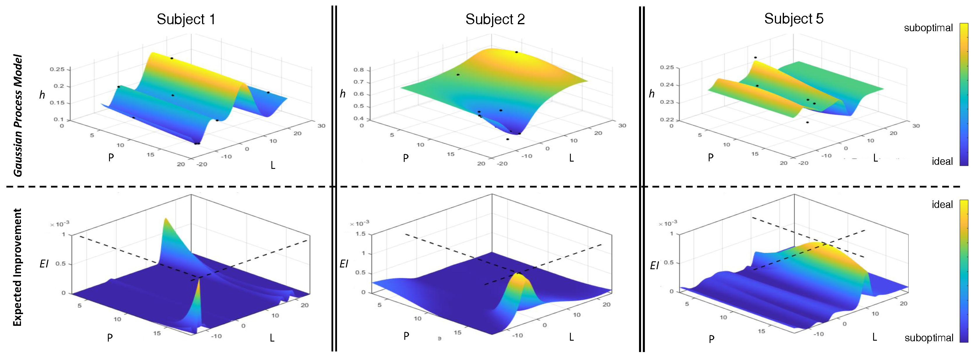

Table 1.
Borg Value Comparison Against Baselines For Validation
| Baseline | Opt. Slow (% change) | Opt. Fast (% change) |
|---|---|---|
| No Device | -26.0% | -14.4% |
| Zero Assistance | -39.5% | -26.8% |
| General Control | -18.5% | 4.9% |
Disclaimer/Publisher’s Note: The statements, opinions and data contained in all publications are solely those of the individual author(s) and contributor(s) and not of MDPI and/or the editor(s). MDPI and/or the editor(s) disclaim responsibility for any injury to people or property resulting from any ideas, methods, instructions or products referred to in the content. |
© 2025 by the authors. Licensee MDPI, Basel, Switzerland. This article is an open access article distributed under the terms and conditions of the Creative Commons Attribution (CC BY) license (http://creativecommons.org/licenses/by/4.0/).
Copyright: This open access article is published under a Creative Commons CC BY 4.0 license, which permit the free download, distribution, and reuse, provided that the author and preprint are cited in any reuse.


