Submitted:
17 January 2025
Posted:
17 January 2025
You are already at the latest version
Abstract
Large-scale data characterized by heterogeneity due to heteroscedastic variance or inhomogeneous covariate effects arises in diverse fields of scientific research and technological development. Quantile regression (QR) is a valuable tool for detecting heteroskedasticity, and numerous QR statistical methods for large-scale data have been developed rapidly. This paper provides a selective review of recent advances in QR theory, methods, and implementations, particularly in the context of massive and streaming data. We focus on three key strategies for large-scale QR analysis: (1) distributed computing, (2) subsampling methods, and (3) online updating. The main contribution of this paper is a comprehensive review of existing work and advancements in these areas, addressing challenges such as managing the non-smooth QR loss function, developing distributed and online updating formulations, and conducting statistical inference. Finally, we highlight several issues that require further study.
Keywords:
Large-scale data
; Quantile Regression
; Distributed computing
; Subsampling methods
; Renewable estimation
1. Introduction
With the rapid advancement of technology, we are entering the era of large-scale data, characterized by the ability to generate and store vast amounts of information at reduced costs. Large sample sizes and high-dimensional features have become defining characteristics of many modern datasets, and the exponential growth of massive datasets across diverse fields has become increasingly common. For example, in genomics, the development of new technologies enables biologists to generate tens of thousands of datasets [1], and the abundance of genomic sequencing data facilitates the identification of genetic markers for rare diseases [2,3]. In economics and finance, an increasing number of companies are adopting data-driven approaches. By analyzing large datasets, such as stock prices and transaction records, companies can better assess risks and make informed decisions [1]. Social networks like Twitter, Facebook and YouTube also generate large amounts of data, enabling researchers to build predictive models that reveal individual characteristics[1,4,5,6]. Although large-scale data can provide richer information for data analysis in various domains, they also pose significant challenges to traditional statistical models [1]. For massive data with both high dimension and large sample size, here we focus on the main techniques that address the following three major challenges.
The first challenge lies in the larger volume of large-scale data. Datasets can reach exabyte-level sizes, yet the memory capacity of a single computer is limited, making it impossible to store the entire dataset. Moreover, traditional statistical models are predominantly built on the assumption that data can be processed on a single machine, such models could be ineffective for large-scale data [7]. To address this challenge, a fundamental strategy for storing and processing such data is distributed learning, often referred to as the “divide-and-conquer” (dc) approach. The idea of dc-method is to partition a massive dataset into smaller data blocks to mitigate memory constraints. A common implementation of this strategy involves compressing subsets of data on each machine into local estimator and then aggregating them on a central host to obtain the final model estimates [7]. In addition, many researchers have explored dc-strategies for various statistical models, such as linear regression [8,9], logistic regression [10], quantile regression [11,12,13], and references therein.
The second challenge arises from the high-speed generation of large-scale datasets. Learning models from such data in a streaming fashion is becoming increasingly ubiquitous, in which data arrive in streams and chunks (also referred to as streaming datasets) [14]. It is often numerically challenging or sometimes infeasible in such a data environment to update the model estimation with the entire dataset in memory. As a result, traditional offline methods, which require access to the full dataset, become less practical or even obsolete. Instead, online methods are capable of providing a way to analyze the out-of-memory data by constructing and updating the model sequentially at one time without storage requirements from previous raw data. The two key issues of streaming data analysis are (1) the storage challenge that old data are already discarded when new data arrive, and (2) the speed challenge that the analysis must be updated in a very fast way to support real-time information processing. Various online methods have been proposed to date, including aggregated estimate equation [15], cumulatively updating estimate equation [16], stochastic gradient descent (SGD) and its variants [17,18], as well as renewable estimators [19]. In this paper, we assume that at a given time point t, only the current data block and the summary statistics based on the previous data blocks are available (see Figure 1). And we focus on the “renewable estimation” or “online updating", which directly update parameter estimates utilizing summary statistics from both previously processed data and newly arriving batches of data [13].
The third challenge is that large-scale data often show heterogeneity due to heteroskedastic variance or inhomogeneous covariate effects [1]. Traditional statistical models are generally predicated on the assumption that the data are homoscedastic and follow Gaussian distributions. However, these assumptions impose significant limitations when applied to the complex structural characteristics of large-scale data. Moreover, most of the existing methods for large-scale data analysis are focused on mean regression models [19,20,21,22,23]. When random error distributions are highly skewed or exhibit heteroskedasticity, linear mean regression models often yield inefficient estimates and poor predictive performance. In contrast, quantile regression (QR) models [24,25] offer a more robust alternative capable of effectively addressing these challenges. By complementing the exclusive focus of classical least squares regression on the conditional mean, QR offers a systematic strategy to examine how covariates influence the location, scale, and shape of the entire response distribution. It has been actively studied in machine learning, economics, finance, and statistics [26,27,28,29,30,31,32,33]. However, these traditional statistical methods for estimating QR models require processing the entire dataset simultaneously. Due to the infinite size of large-scale datasets and the limited memory capacity of computers, these conventional parameter estimation methods are not applicable [7]. While there has been substantial research on distributed learning algorithms and online updating algorithms for large-scale data [16,19,34,35], the non-differentiability of the objective function in quantile regression makes it challenging to directly adapt these algorithms for estimating quantile regression models.
Therefore, this paper provides a comprehensive methodological framework for QR in the context of large-scale data as shown in Table 1. Specifically, the main contributions of this overview are summarized as follows:
- Overcoming non-differentiability of the QR check function. We introduce common techniques on smooth or surrogate of the QR loss function.
- Parameter Estimation in distributed and streaming settings. We systematically reviewe methods to efficiently compute and aggregate QR estimates when large-scale data is stored across multiple machines or in one machine. Then we summarize recent research progress of renewable estimation for QR regression as the data arrive sequentially.
- Statistical Inference for Large-Scale QR. We briefly introduce statistic theoretic of QR estimator for large-scale data, such as asymptotic distribution and techniques about how to derive empirical variance of estimators.
- Applications. We introduce the applications in meteorological forecasting, demand and price forecasting, geographical distribution data and high-frequency data forecasting.
- Potential research directions. We provide some potential research directions which can promote the development of this field.
Due to space limitations, we primarily focus on the linear QR framework when reviewing existing work on large-scale data. We do not evaluate each method in detail, however, we will offer guidance on the scenarios where specific methods are most effective and discuss the potential for further advancing the existing literature to tackle emerging challenges in large-scale data quantile regression analysis.
The rest of this article is organized as follows. Section 2 briefly reviews the foundations of QR. Section 3 and Section 4 illustrate advances on QR for massive data and streaming data, respectively. Section 5 introduces the applications of QR for large-scale data. Limitations and potential future work are discussed in Section 6.
2. Foundations of Quantile Regression
In this section, we first show the definition and mathematical framework of QR in Section 2.1. Then, we introduce some common estimating techniques in Section 2.2. Finally, we summarize the key differences and advantages compared with mean regression in Section 2.3.
2.1. Definition and Mathematical Framework of QR
A basic tool in different scientific fields for analyzing the impact of a set of regressors X on the distribution of a response Y is QR, and it can be defined with the help of appropriate loss functions. For a fixed , the th conditional quantile of Y given X, , can be obtained by minimizing asymmetrically weighted mean absolute deviations [24]:
where is the check function as shown in Figure 2, and is the indicator function. Observably, is the piecewise linear function and is the absolute loss function. Note that subtracting from the expectation as shown in (1) makes the integrand well defined and finite without assuming .
Let be i.i.d. samples draw from , then the linear QR model follows:
where and is the unknown quantile regression coefficients. The QR estimator can be obtained via minimizing the following objective function:
Besides estimation, statistical inference for QR is also a critical aspect. Basically, it involves constructing confidence intervals, hypothesis testing and assessing the variability of the estimated parameters, etc. The central work for statistic inference is to derive the asymptotic distribution of the QR estimator as . Assume and are the conditional cumulative distribution function and the density function of , which satisfies . As was shown by Koenker and Bassett [24], under some regularity conditions, is asymptotically normal:
where , and denotes convergence in distribution. Although the asymptotic covariance matrix seems to suggest that estimation of regression quantiles becomes increasingly more precise when very small () or large () quantiles are considered (due to the product in the numerator), in fact this effect is typically dominated by the error which will usually be close to zero for such values of . Hence, the estimation of interior quantiles close to the median will actually be more precise for most of the standard distributions, while estimation of outer quantiles is associated with larger uncertainty.
Here the sample estimation of the covariance matrix denotes as:
where is the conditional density estimator of evaluated at 0. Note that the asymptotic variance of QR estimator involves density function of the error terms, which is unknown generally. Thus, direct implementation via the asymptotic variance is difficult. Generally, an alternative inference would be based on bootstrap method. Please refer to Chapter 3 of Davino et al. [36] for more details. For simplicity, we will omit of or in the following paper whenever there is no ambiguity.
2.2. Common Estimation Techniques
Estimation of QR parameters typically involves solving an optimization problem to minimize the check function in (3). This function is nondifferentiable, which poses challenges for direct computation. Figure 2 illustrates the check function at a specified level , highlighting the nondifferentiability of the loss function at . The QR estimation can mainly be classified into three types: (1) linear programming (LP) method; (2) smooth QR method, and (3) Bayesian QR method. We summarize them together with the main algorithms in Figure 3, which are briefly discussed below.
Linear programming technique expands the estimation problem by introducing auxiliary variables and with , where and therefore with . The minimization problem (3) can be rewritten as
where is a unit vector. This is a constrained minimization problem with polyhedric constraints, i.e., the constraint defines a geometric object with flat faces and straight edges, such that the constrained problem corresponds to the original quantile restriction, but written in terms of the auxiliary variables. After augmenting the auxiliary variables and given the constraints, the minimization problem is now linear in the parameters and can therefore be tackled with linear programming techniques that allow to incorporate the polyhedric constraints. Refer to Lange [37] for a brief introduction to linear programming with a focus on statistics-related applications. By reformulation, (5) can be solved by simplex methods [38] or interior point methods [39].
Algorithms developed for the general LP problems in (5) may not fully deploy the properties of or quantile regression and have their own shortcomings. For example, the interior point algorithm can only give the approximate solutions of the original problem, and rounding is necessary to provide the same accuracy as that of the simplex algorithm. In this case, some heuristic approaches demonstrate the advantages of both speed and accuracy. One such approach is the smoothing method, which aims to approximate the objective function in (3), enabling the use of Newton or quasi-Newton optimization methods. There are three main types of smoothing techniques: 1) Horowitz’s smoothed loss [40,41]; 2) Huber’s smoothed loss [42] and 3) Convolution-type smoothing [43,44,45,46].
More specifically, Horowitz’s smoothed loss approximateds the indicator function with a smooth function , where takes values between 0 and 1, and is the bandwidth. For example, can be chosen as the distribution function of standard normal . With this approximation, one can replace by
Instead, Huber’s smoothed method approximated by the generalized Huber function , i.e.,
where is a threshold. Different from the former, the convolution-type smoothing method approximates with a smooth function , i.e.,
where ∗ denotes the convolution operator, and throughout the paper, with being a kernel function that integrates to one and being a bandwidth. Following He et al. [44], we adopt the term conquer for convolution-type smoothed quantile regression.
Thus, the corresponding smoothed QR estimator can be obtained via the empirical smoothed loss function in (6)-(8), respectively. In Section 3 and Section 4, we show how these smoothing techniques used in the large-scale setting.
The third option for QR estimation is Bayesian approaches, which utilize the Asymmetric Laplace distribution (ALD) as a likelihood function [47,48]. Let be the ALD with location parameter , scale parameter and asymmetric (skewness) parameter , and the pdf is given by
This method imposed the , on the residual terms, hence the cumulative distribution function of is , then . Thus, the likelihood is reformatted as:
For estimation, given a prior distribution of , the Gibbs sampler can be used to derive the Bayesian QR model. In addition, the EM algorithm can also be applied to estimate in (9) due to the fact that a mixture representation was developed for the ALD based on a normal variance–mean mixture with an exponential mixing distribution. More details can be found in Kozumi and Kobayashi [48].
Comparing the aforementioned estimation algorithms, the LP algorithm faces significant computational challenges when applied to large datasets. In contrast, smooth QR and Bayesian QR methods benefit from the continuity of their loss functions, and it is easy to derive iterative algorithm or closed-form estimators. These properties make them more adaptable to modern computational strategies, such as distributed and online algorithms, which are often employed to manage the growing complexity of data in practical applications. Finally, we list some standard QR packages, which can be found in R (with the “quantreg” package), SAS (through the “PROC QUANTREG” procedure), Python (via “statsmodels” library and QuantReg class), Matlab (with the “quantreg” function) and STATA (using the “qreg” command).
2.3. Comparison with Mean Regression: Key Differences and Applications
Quantile regression goes beyond modeling the conditional mean and provides a detailed representation of the entire conditional distribution. This makes QR particularly valuable in a wide range of applications, with its advantages evident in the following key aspects: (1) robustness, (2) interpretability, and (3) flexibility.
More specifically, unlike traditional mean regression, which minimizes the mean squared error and assigns equal weights to all samples, QR is less sensitive to outliers. This robustness arises because QR minimizes the check loss function, which adjusts the influence of data points based on their position relative to the quantile being estimated. Moreover, by analyzing the effects of predictors across different quantiles, QR effectively captures heteroskedasticity, outliers, and skewed distributions in the data. This ability to offer insights into multiple aspects of the data distribution enables QR to deliver a more nuanced and reliable analysis compared to traditional mean-based regression methods. For example, in the medical field, anesthesia research is a significant area of study. However, related variables, such as the length of hospital stay, ventilator dependence, blood loss, and pain scores, often violate the assumptions of normally distributed residuals, homoskedasticity, and independence. Relying solely on linear regression in these cases can result in inaccurate model estimates. To address this issue, Staffa et al. [49] applied multivariable quantile regression, which provides a more comprehensive and accurate understanding of the relationships between risk factors and outcomes.
Besides robustness, interpretability means that QR offers a comprehensive view of the effects of explanatory variables at different quantile levels. Many studies show that QR provides more insights than mean regression. For example, in non-Gaussian data distributions, QR improves model accuracy and is widely used in market return studies [50,51,52]. It also reveals weight change trends among different groups in U.S. girls’ weight and age studies [53]. In medical research, QR uncovers differences in the relationship between ventilator dependence and hospital stay across quantiles [49]. In ecology, QR provides a more complete view of causal relationships, as shown in studies linking trout abundance to stream width-to-depth ratios [54,55]. Empirical results indicate that mean regression might incorrectly suggest no relationship between trout density and stream ratios.
Lastly, in cases where data is missing or observed values are biased from actual values, QR effectively mitigates the impact of missing data on model fitting [56]. For instance, in ecological research, scholars have noted that when ecological limiting factors constrain organisms [55], many other unmeasured ecological factors may also impose limitations on biological responses. This makes mean regression insufficient for capturing the true patterns of biological responses. In contrast, QR can estimate the upper limits of biological response potential without being affected by unmeasured factors. Cade [57] explored in greater detail the multiplicative interactions between measured and unmeasured ecological factors and addressed the aforementioned analytical issues using QR methods.
3. Advances in QR for Massive Data
In this section, we briefly introduce foundational work on QR for massive datasets. In such situations, the size of the dataset can become so large that the storage of it on a single machine is impractical. Additionally, traditional methods often become infeasible due to the significant computational burden. In the following section, we focus on two common approaches for handling massive data: (1) distributed computing and (2) subsampling methods in Section 3.1 and Section 3.2, respectively. We also discuss the scenarios in which each of these methods is most effective. A summary is provided in Table 2.
3.1. Distributed Computing
Distributed computing (dc) is a computing paradigm in which a single system’s tasks are divided across multiple independent computing nodes that work collaboratively to achieve a common goal. These nodes, often geographically dispersed, communicate and coordinate their works through a network. A related concept is the dc framework [22,58,59,60], which breaks down a problem into smaller sub-problems, solves each problem independently, and combines their results to derive the overall solution. And this concept has already been applied in practice by many scholars [23,61,62,63].
For large-scale datasets, we below describe a general dc algorithm for QR estimation. Assume the entire samples follows (3), we split the data indices into K subsets with each size , that is . Correspondingly, the entire data set is divided into K batches , where for .
During estimation, each data batch is stored on a single machine and a low-dimensional statistic is computed in each subset . These statistics are transformed to main machine and then aggregated using an aggregation function, to obtain the final global estimator.
The dc framework is often implemented through two methods, one-shot (os) and communication iterative computation, see Figure 4. Specifically, the os computation refers to a process where tasks are distributed and solved in a single computation, with all nodes working independently before that their results are aggregated [23]. This approach is efficient for problems that do not require intermediate communication or feedback between nodes during processing. For instance, Lee et al. [64] proposed a simple and communication-efficient method for distributed high-dimensional sparse regression based on the os approach.
While the os computation can be efficient for simple or well-structured problems, it lacks efficiency in terms of data utility. If the initial estimation is suboptimal or inaccurate, there is no built-in mechanism for adjustment or improvement. Hence it is highly sensitive to noise, errors, or biases in the input data, which can significantly impact the final result. To improve the statistical efficiency of os estimators, distributed communication iterative methods have been proposed [65,66]. Compared to the os method, communication iterative methods make more comprehensive use of global information, leading to more precise parameter estimation.
In the follow part of this section, we will discuss some seminal research about implementation of QR for distributed computing.
3.1.1. One-Shot Method and Its Variants
os is the simplest distributed method, requiring only that parameters be estimated on local machines and then transmitted back to the master for averaging/aggregate to obtain the final global estimates. Specifically, for each data batch, we first estimate local parameter in (3) using kth batch samples . Each local parameter is then sent to the master, which calculates the global estimator by , which is denoted as the os estimator .
Extensive research has been proposed in this field for QR. For example, Xu et al. [63] developed a block average approach, employing the os strategy by averaging estimators derived from each local computer.
Chen and Zhou [7] also applied the os strategy by reconstructing the estimator for the entire dataset with an asymptotically negligible approximation error. Moreover, this method not only introduces a resampling technique that simplifies and enhances the efficiency of weight matrix computation, but also yields a global estimator in closed form by combining low-dimensional statistics derived from each data block. This feature further facilitates continuous model updating in streaming data scenarios.
To guarantee statistical efficiency, Volgushev et al. [67] proposed a distributed quantile curve estimation method based on a two-step quantile projection algorithm. First, they estimated specific -quantile values (i.e., ) in local machine and aggregated them to the master, which outputs a pooled estimator; then, they applied a B-spline method to construct a projection matrix for generating the overall quantile curve. More specifically, let,
where is a B-spline basis defined on equidistant knots. Then the quantile curve can be obtained by , where is the projection matrix. This method can be applied to the inference of conditional distribution functions, enabling researchers to better understand the distributional characteristics of the data. Furthermore, due to its use of subsample estimators for computation, it offers low computational cost, making it more suitable for practical application scenarios.
The drawback of the aforementioned research is that relies solely on local information, which can lead to statistical inefficiency, particularly when the data are not randomly distributed between workers. To address this issue, Pan et al. [68] proposed an updating algorithm. Based on the following asymptotic expression of global estimator,
where denotes convergence to zero in probability. And the one-step update estimator derived by replace in (10) by a pilot estimator (eg. estimator derived in node ) and . That is,
where is a kernel density estimator.
3.1.2. Communication Iterative Computation
Communication iterative computation, on the other hand, involves multiple iterations of computation and communication. In this approach, nodes repeatedly update their results based on feedback or inputs from other nodes, gradually converging toward the final solution. This strategy utilizes information from the entire dataset, leading to significantly improved accuracy compared to the os strategy. However, communication iterative computation requires data transmission among multiple machines, which can result in high communication costs. Balancing statistical efficiency with reduced communication overhead has therefore become a critical challenge in this area of research. Additionally, in the QR framework, the non-differentiability of its loss function poses another significant challenge. This makes it impossible to directly apply the communication loss function. Consequently, the critical issue in distributed computing for QR is how to approximate or derive the gradient function for a non-differentiable loss function, together with excellent statistical efficiency with well-controlled communication costs. Below we review some related work.
One notable work in this regard is motivated by the communication-efficinet surrogate likelihood method proposed by Jordan et al. [65], and extend it to QR [45,69]. The differences between them are the different techniques for the non-smooth nature of the QR loss function. For example, Hu et al. [69] introduced sub-gradients to construct a surrogate loss function, and established the consistency and asymptotic normality of the proposed methodology. Later, Tan et al. [45] applied the convolution smoothing approach (8) to the local and global objective functions of quantile regression.
Beyond the above work, researchers address the challenges of distributed QR by proposing various loss functions via smoothing techniques introduced in Section 2.2 and iterative algorithms. For example, Chen et al. [41] presented a computationally efficient method based on Horowitz’s smoothed loss in (6), which involves multiple rounds of aggregations. Specifically, for the k-th batch,
Here is the derivative of , and is the estimator from the -th iteration, and update the estimator at the -th iteration as:
After limited q iterations, the authors show that the statistical efficiency of the final estimator becomes the same as the one computed on the whole data. They also designed a new one-pass algorithm for streaming data. For more details, please refer to Chen et al. [41].
Note that gains smoothness at the cost of convexity, He et al. [44] and Tan et al. [46] employed the convolution-type smoothing loss in (8), which transforms the loss function into a convex and twice-differentiable form. Their work focuses on statistical inference for QR in the context of the “increasing dimension". For massive data, Jiang and Yu [70] proposed smoothing QR for a distributed system based on the conquer approach and its Taylor expression. Specifically, via (8), the empirical smoothed loss function becomes,
and the smoothing estimator is given by .
Note that the entire data are located in K local machines, each machine cannot communicate to the master machine, then Jiang and Yu [70] adopted a Taylor expansion of around an initial estimator , yielding:
where and are the gradient and Hessian matrix:
where . Note that (15) is a convex quadratic loss function, thus under a distributed system, and can be rewritten as:
where . To avoid communication cost, similar to Jordan et al. [65], one can replace with , and the convolution-type smoothing QR can be derived by Newton-Raphson algorithm, i.e., , where is the Hessian matrix with bandwidth which selected base on the first machine. Moreover, Jiang and Yu [70] also extended the above distributed smoothing QR estimator in high dimensions by incorporating penalty. For more details, please refer to Jiang and Yu [70].
3.1.3. Distributed High-Dimensional QR
Modern data acquisitions have facilitated the collection of massive and high-dimensional data, here we briefly summarize some work related QR under massive and high-dimensional data [67,70,71,72,73,74]. For example, Volgushev et al. [67] studied a os QR method with fixed or growing dimension; Zhao et al. [71] proposed a bias-correct method [75] to obtain a de-biased estimator before taking the averaging. However, the de-biasing step is computationally time-consuming and suffers the drawbacks of the os method. Wang and Lian [72] extended the communication-efficient surrogate likelihood method proposed by Jordan et al. [65] for distributed QR, while Chen et al. [73] transformed QR loss to a least squares loss and provided a distributed estimator that is both computational and communicatively efficient. Recently, motivated by Chen et al. [73], Wang and Shen [74] extended Tan et al. [45] to high-dimensional setting, proposed a novel method for distributed high-dimensional QR. Overall, different from distributed estimation in Section 3.1.1 and Section 3.1.2, support recovery or variable selection is also a task. One notable practice is to incorporate the penalty function, such as proposed by Tibshirani [76] and smooth clipped absolute deviation (SCAD) proposed by Fan and Li [77].
3.1.4. Distributed Statistical Inference for QR
In addition to estimation, other statistical inference tools, such as hypothesis testing and confidence intervals, also play a crucial role in scientific research and data analysis. These inference tools allow researchers to quantify the uncertainty of the estimators obtained from the data, and then help practitioners interpret the results appropriately. In the above discussion of this section, various distributed estimation methods have been introduced. Thus, we briefly summarize some attempts on the statistical inference for distributed QR.
In fact, there have been potential challenges for the statistical inference of the standard QR. Classical approaches to inference are typically based on estimating its asymptotic variance from the data directly, or conducting bootstrap to approximate the asymptotic distribution. First, estimating the limiting variance requires the choice of a bandwidth parameter, and existing research indicates that classical rules for bandwidth selection need to be adjusted in a dc setting [78]. For example, Pan et al. [68] proved that in (11) shared the same asymptotic distribution with the global estimator, i.e., (4). Thus, they performed valid statistical inference with non-parametric estimator of and a standard moment estimator of , which can be estimated easily on a distributed system. Second, the bootstrap approach requires repeatedly computing QR estimates up to thousands of times, and therefore is unduly expensive for massive data inevitably. To solve this problem, Volgushev et al. [67] proposed several simple inference procedures which directly utilize the fact that in a dc setting, estimators from subsamples are available. Their procedures are very easy to implement and require only a very small amount of computation on the central computer without additional communication costs. Please refer to Volgushev et al. [67] for more details.
There are also some work related to large-scale statistical inference for QR without in the distributed framework. For example, He et al. [44] propose a bootstrapped procedure to perform hypothesis testing and confidence estimation with larger dimension and larger sample size. Later, Lee et al. [79] developed a fast inference procedure for QR with ultra-large dataset based on stochastic subgradient descent (S-subGD) updates. The inference procedure handles cross-sectional data sequentially: (i) updating the parameter estimate with each incoming “new observation", (ii) aggregating it as a Polyak–Ruppert average, and (iii) computing a pivotal statistic for inference using only a solution path.
3.2. Subsampling-Based Method for QR
Distributed algorithms provide an effective solution for statistical modeling with massive datasets. However, they face several challenges in practical applications: 1) high cost of distributed computing systems and 2) high learning cost. As an alternative approach, subsampling repeatedly generates small subsamples for parameter estimation and statistical inference, which has been widely used to reduce the computational burden when handling massive data. It performs analysis on a small subsample drawn from the full data and provides a practical solution to extracting information from massive data with limited computing power. Consequently, various subsampling methods are proposed, and has been applied for linear regression [80,81,82], logistic regression [83,84] and generalized linear regression [85,86]. Existing optimal subsampling techniques require a differentiable objective function or loss function, hence traditional subsampling strategies can not be applied directly to QR. Below we describe some work on subsampling-based methods for QR [21,86,87,88].
For example, Wang and Ma [87] studied optimal subsampling procedures and derived the asymptotic distribution of a general subsampling estimator and two versions of optimal subsampling probabilities. Specically, taking a random subsample using sampling with replacement from the full data satisfying (3) according to the probabilities , such that . Denote the subsample as , with associated subsampling probabilities . The loss function of subsampling QR denote as:
The subsample estimator, denoted as , is the minimizer of The asymptotic normality of has been established, which can be used to identify the optimal probabilities by minimizing the trace of the asymptotic variance-covariance matrix, either for a linearly transformed parameter estimator, or the original parameter estimator. See Theorem 1-3 in Wang and Ma [87]. Later on, subsequent studies have also validated the effectiveness of this approach [89], which proposed a weighted least squares resampling approach for estimating the variance-covariance matrix of QR subsample-based estimator.
The subsampling methods mentioned above primarily focus on the weak convergence of the resulting estimator, which often fails to effectively capture the convergence rate. Consequently, the theoretical framework does not offer clear guidance on determining the appropriate subsample size. To address this, Ai et al. [86] proposed a Poisson sampling QR method for large-scale data, where subsamples are selected through independent Bernoulli trials to approximate the full dataset. This method eliminates the need to calculate sampling probabilities in RAM all at once, thereby significantly reducing computational costs when dealing with extremely large datasets. Beside, when the dataset cannot be stored on a single machine, a single optimal subsampling procedure becomes inadequate for addressing such distributed scenarios. To overcome this issue, Chao et al. [88] proposed a distributed QR subsampling procedure, and developed the optimal subsampling probabilities and subset sizes selection criteria simultaneously via a two-step algorithm. The theoretical results, such as consistency and asymptotic normality of resultant estimators are established.
4. Advances in Quantile Regression for Streaming Data
In contrast to Section 3, here we focus on studies for QR for streaming data. As mentioned in the Section 1, streaming data consist of data blocks arriving sequentially over time, and it requires frequent updates to the analysis result as new data is collected. However, due to the sheer volume of data, it also becomes challenging to store all the information from each batch. As a result, renewable estimation or online updating methods have been proposed, as shown in Figure 1. Here we first introduce some notations used in this section. Assume are aggregated streaming data up to batch b, where are the streaming data of t-batch with sample size satisfying (3), i.e.,
And the total sample size is . For simplicity, in this section, we omit whenever there is no ambiguity, and use “” to denote the online estimator (i.e., is the renewable estimator obtained via data up to batch b, ) and “” to denote the estimates derived from data at stationary time points (i.e, obtained via data from ), respectively.
The core challenge of streaming QR lies in constructing a renewable estimation framework that allows parameters to be updated incrementally as new data arrive, without the need to store or reprocess the entire dataset. Existing methods for renewable estimation for QR can be categories into three types: (1) the one-shot divide-and-conquer algorithms (os-dc) as well as its variants when viewing stream data as data blocks partitioned over the time domain; (2) sequential QR (sqr) algorithm partly motivated by Bayesian QR; and (3) the cumulative estimating equation together with a Taylor expansion method (cee-taylor). Table 3 summarizes these three types of renewable algorithm, and we will introduce the above three strategies in detail in the following sections.
4.1. os-dc Methods and Its Variants
Note that most of these techniques in Section 3.1.1 and Section 3.1.2 are only applicable to static big data but not stream data except the os-dc algorithms when viewing stream data as data blocks partitioned over the time domain [23,41]. For example, Chen et al. [41] applied Horowitz’s smoothing QR for streaming data by using the dc strategy via a one-pass algorithm (see Algorithm 2 in Chen et al. [41]) to provide a sequence of successively refined estimators. While the os-dc algorithms can be naturally extended to stream data by implementing the aggregation in a block-by-block manner, it often requires the block size to grow to infinity to establish their asymptotic theory. However, the block size in stream data is generally determined by hardware capacity and hence fixed. In addition, updates based on direct applications of os-dc algorithms may not be efficient enough to support the frequent update in the stream data context.
As a straightforward extension of the os-dc technique, Wang et al. [11] developed an updating estimator based on the normal approximation of the QR estimator from a single batch of data. Based on its asymptotic distribution, the local QR estimator can be treated as sample generated from the following multivariate distribution:
where with being the pdf of error term, and for . Then, based on the multivariate normal distribution, the renewable estimator can be formulated as:
where . Obviously, in order to run the renewable algorithm (18), one only needs to store for each batch of data, while the historical data are not completely involved. The idea of Wang et al. [11] has been extended to other complex regression problems, such as expectile regression [96], Huber robust regression [97,98], unconditional quantile regression [99] and composite quantile regression [95].
Unlike Wang et al. [11], Chen and Zhou [7] also proposed a simple and efficient dc-based strategy for the estimation of the QR model with massive datasets, which only keeps compact statistics of each data block and uses them to reconstruct the estimator of the entire data, with an asymptotically negligible approximation error. This property makes the proposed method particularly appealing whenever the data blocks are retained in multiple servers or received in the form of data stream. Specifically, for the data up to batch b, the proposed renewable estimator can be formulated in the closed-form:
where is the estimator of , which is estimated via a resampling method inspired by Zeng and Lin [100]. Here is the conditional density function of Y given X.
4.2. sqr Algorithm
Note that local processing in Zhang et al. [23] and Wang et al. [11] requires solving a QR problem, which results in updates that are too slow for real-time processing of stream data. Recall that Bayesian QR uses a linear model with an ALD error term to achieve equivalence between the original QR estimator and the Bayesian maximum-a-posteriori (MAP) estimator [47]. Additionally, the scale-mixture representation of the ALD holds [48]. Motivated by these foundations, Fan and Lin [12] proposed a sqr algorithm, where sequential updates occur naturally within the Bayesian setup. Specifically, the posterior distribution obtained from the past analysis is used as the prior information for later analysis.
The data block arriving at time point is denoted as . They first converted the check loss optimization based on each data block to a least squares problem to expedite local processing to accommodate the frequent update in stream data, resulting in ; the sqr estimator is then updated up to batch b, denoted as . This estimator is calculated by solving a nonzero centered ridge regression problem [101], which has a closed-form solution given as follows:
From a theoretical perspective, the proposed estimator is asymptotically normal and achieves a linear convergence rate under mild conditions. Additionally, the computational complexity is significantly reduced from to , offering a notable improvement over distributed algorithms. The general idea of sqr has also been extended to composite quantile regression [102]. Please see Algorithm 1 in Fan and Lin [12] for more details.
Similarly, Tian et al. [90] also proposed a Bayesian QR approach for streaming data, in which the posterior distribution was updated by utilizing the aggregated statistics of current and historical data. Leveraging the posterior distribution of historical data as the prior for current data stream, a posterior distribution is established without any loss of information, which ensures that the proposed Bayesian streaming QR estimator is equivalent to the global oracle estimator calculated based on the entire data.
4.3. cee-taylor-Based Renewable Estimation
For massive data, the cumulative estimating equations estimator was proposed first by Lin and Xi [15] and subsequently adapted to the sequential estimation setting by Schifano et al. [16], yet their estimation consistency may not be guaranteed in the situation where streaming datasets arrive perpetually with . To overcome this unnatural limitation, Luo and Song [19] presented an incremental updating algorithm to analyze streaming datasets using generalized linear models. The main procedure can be summarized as follows.
Denote and as the general aggregated loss function based on data up to batch b (i.e., ) and data at batch b (i.e., ), respectively. First, decompose into a combination of the historical data and the arrival of new data, i.e.,
Then, by applying Taylor expansion to the first part of (21) around the online estimates up to batches, , can be asymptotically equivalent to (omitting terms that do not contain the unknown parameter):
where is the second order function of of t-th batches. Then the renewable estimation based on data up to batch b is defined as a minimizer of (22). We adopt the term cee-taylor-based renewable estimator for the above procedure.
Extensive researches have extended the idea of cee-taylor to QR for streaming data by incorporating the smoothing techniques to ensure that the objective function remains both differentiable and convex [91,92,93,94]. For example, both Jiang and Yu [91] and Xie et al. [93] proposed a renewable method for QR via the convolution-type smoothing objective function:
where with defined in (8). Then the proposed renewable estimator at bacth b can be obtained according to (21) and (22) with replaced by . That is, the the renewable estimator up to batch b, , is given by:
Moreover, Xie et al. [93] proposed a online high-dimensional smoothed-type QR algorithm. For variable selection, this paper replace in (23) with the following lasso estimator:
where is the regularization parameter adaptively selected after the arrival of the b-th batch data. Additionally, an online debiased lasso procedure is developed for inference, where the debiasing matrix is computed using only the current data and summary statistics from previous batches. For theoretical respect, the proposed online estimators enable efficient estimation and valid inference. For further details, refer to Xie et al. [93].
In addition to the convolution-type smoothing objective function, Horowitz’s smoothing method could also be adopted for QR renewable estimation. Note that achieves smoothness at the cost of convexity. To address this issus, Sun et al. [92] introduced a convex smooth quantile loss, which is infinitely differentiable and converges uniformly to the quantile loss. Specifically, they modified by adding and proposed the following loss
where is nonnegative bounded function satisfying . Then following the same procedure in CEE-Taylor-based renewable estimation described in (21) and (22) with replaced by the smoothing loss function in (24). Later, Peng and Wang [94] also adopted the Horowitz’s smoothing method to propose a two-stage online debiased lasso estimation and statistical inference method for high-dimensional QR models in the presence of streaming data. For more details, please refer to Sun et al. [92] and Peng and Wang [94].
4.4. Renewable Estimation for Streaming Quantile Eegression Under Heterogeneity Scenario
Most existing online learning methods are based on homogeneity assumptions, which require the samples in a sequence to be independent and identically distributed (i.i.d.). However, as data are generated over time, maintaining homogeneity between different batches becomes increasingly challenging, especially as the growth of number of batches and intervals between data collections. This suggests that different batches may not necessarily originate from the same underlying model. In fact, batch correlation and dynamically evolving batch-specific effects are key characteristics of real-world streaming data, such as electronic health records and mobile health data. As a result, research into online updating methods that address heterogeneity has become an emerging and significant area of study.
For example, Luo and Song [103] studied multivariate online regression analysis with heterogeneous streaming data for linear regression, while Wei et al. [104] proposed a new online estimation procedure to analyze the constantly incoming streaming datasets in the framework of generalized linear models with dynamic regression coefficients to address potential heterogeneity. Recently, Ding et al. [105] studied renewable risk assessment of heterogeneous streaming time-to-event cohorts, where risk estimates for each cohort of interest are continuously updated using the latest observations and historical summary statistics. They introduced parameters to quantify the potential discrepancy between batch-specific effects from adjacent cohorts and applied penalized estimation techniques to identify nonzero discrepancy parameters, adaptively adjusting risk estimates based on current data and historical trends.
Similarly, for QR with heterogeneous streaming data, Chen and Yuan [13] developed an online renewable QR method with streaming datasets, respectively under the homogeneity and heterogeneity assumptions. The renewable strategy is based on the cee-taylor approach, and a homogeneity detection method was proposed to identify potential homogeneous parameters that are the same for all data batches through penalized estimation.
5. Application
In the previous sections, we introduce some seminal work for QR for large-scale data, including the model setup, parameter estimation algorithm, and statistical inference. In this section, we aim to introduce the application fields for large-scale QR in detail and introduce some benchmark datasets.
5.1. Meteorological Forecasting
One key application field of large-scale QR is predicting air quality or pollutant emissions. Meteorological data typically exhibit the following characteristics: First, such data are often collected from various monitoring stations, resulting in decentralized storage. Second, because sensors are generally placed in diverse geographical locations, the collected data tend to exhibit heterogeneity due to natural geographical differences. Lastly, meteorological data are typically collected at high frequencies, such as hourly or even by the minute, leading to a massive volume of data. Consequently, retaining all historical data may sometimes be infeasible, creating a streaming data scenario.
Chen and Zhou [7] applied distributed computing methods to study the factors influencing PM2.5 emissions in Beijing. Their dataset contained hundreds of thousands of observations. The empirical results indicated that distributed algorithms could achieve the same accuracy as oracle (pooled) estimation while significantly reducing data transmission and computational costs. Furthermore, QR enabled the model to better capture the heterogeneous effects of independent variables on the response variable. In contrast, Wang et al. [11] employed a renewable approach to build a QR model for forecasting greenhouse gas (GHG) emissions. Below we list a dataset, sourced from the University of California, Irvine Machine Learning Repository (UCI/GHG), contained over a million data points. Due to large volume of dataset, storing all historical data for subsequent analysis was impractical. Empirical results demonstrated that the online updating method performed comparably to the oracle QR.
5.2. Demand and Price Forecasting
The second empirical research scenario for large-scale QR is in the consumer market forecasting. Compared to other fields, the consumer market has the following characteristics: First, demand in consumer markets is often highly asymmetric, significantly influenced by extreme events such as promotions and holidays, which can lead to substantial fluctuations. Second, consumer market data typically comes from multiple sources, including online transactions, offline sales, social media feedback, and market surveys, resulting in enormous data volumes. Lastly, consumer markets are susceptible to outliers, such as seasonal changes or sudden events, which can significantly affect forecast results. As mentioned earlier, QR can capture different quantiles of distributions, providing a more precise description of demand fluctuations. Hence, it is generally more robust compared to conditional mean regression.
Pan et al. [68] applied subsampling method to predict vehicle prices based on QR. The dataset is from the Kaggle US Used Cars dataset (Kaggle). In the empirical analysis, 28 factors were selected to assess car prices and evaluate computational costs. The results showed that even with millions of data points transmitted during the analysis, the communication cost remained acceptable. Fan and Lin [12] applied the online updating algorithm to forecast prices using the same dataset. The results were consistent with reality experiences, cars with higher horsepower and lower mileage are more likely to be sold at higher prices. Additionally, by comparing the computational speed between online updating method and distributed computing, the online updating method reduced computation time by . Xie et al. [93] used the Seoul Bike Sharing Demand dataset for demand forecasting with renewable estimation algorithm (UCI/bike). The study found that temperature had a negative effect on bike rentals during the winter (lower quantiles) but a positive effect in other seasons. This is expected because people are less likely to rent bikes when temperatures are relatively low in winter.
5.3. Geographical Distribution Data
Another common application of large-scale QR is geographical data, where data storage distributed by geographical divisions. Such data typically comes from multiple sources, and with distributed algorithms research can build model in parallel, improving computational efficiency. Additionally, because of the natural geographical segmentation, data collection often faces uneven spatial distribution and heterogeneity. QR can significantly enhance the robustness of model fitting.
Huang et al. [106] used an iterative communication distributed algorithm to conduct large-scale QR on wine quality data (UCI/wine) and geological data from Xuchang. The study found that, due to the heterogeneity of data from different geographical locations, the iterative distributed quantile regression performed significantly better than the one-shot method and achieved prediction accuracy comparable to the oracle method.
5.4. High-Frequency Data Forecasting
The fourth application of large-scale QR is in high-frequency data, characterized by large volumes, rapid changes, and high real-time demands. This type of data is commonly observed in aviation, financial markets, and electrical load monitoring. For instance, aviation data includes real-time flight positions, speeds, weather conditions, and delays, all of which require timely analysis for effective decision-making in the aviation industry. In financial markets, stock prices, trading volumes, foreign exchange rates, and futures prices can fluctuate on a millisecond basis. Financial institutions rely on analyzing such data for high-frequency trading, risk management, and market monitoring. These data types often exhibit significant uncertainty and volatility, which traditional mean regression methods fail to adequately capture. In contrast, QR provides a more comprehensive view of the data distribution, allowing it to account for the effects of outliers and extreme events more effectively.
Sun et al. [92] built a prediction model on household electricity usage prediction, with data sourced from UCI/electric. The empirical results showed that the prediction results with renewable algorithm achieved same accuracy as oracle estimation and even with very small batch sizes, the final model prediction accuracy remained largely unaffected. Xie et al. [93] applied the proposed method to assess the stock returns of the CSI 300 Index. The prediction results showed that the renewable estimator produced stable results and led to reliable conclusions. The study also suggested that, in practice, financial managers may track stocks over a longer period and cautiously construct portfolios to ensure stability, and that the online updating method could be an effective tool for analyzing stock datasets. Chen and Yuan [13] studied the influence factors of flight delays, the data available at www.transtats.bts.gov. The empirical study demonstrated that the online updating algorithm effectively reduced the computational costs of parameter estimation. Additionally, the proposed heterogeneity detection method was able to capture dynamic parameter changes between different batches, better uncovering the heterogeneous information in the data.
6. Concluding Remarks and Future Research
This paper provides a selective review of QR methods for large-scale data, addressing both static datasets with massive size (massive data) and streaming data. First, we revisited some foundational work on QR, focusing on the common smoothing techniques to overcome the non-differentiability of the QR loss function. Next, we reviewed the development of QR for massive data, which includes one-shot method and its variant, communicative iterative methods and subsampling-based methods. In addition to estimation techniques, we also summarized developments in distributed high-dimensional QR and distributed statistical inference. Subsequently, we discussed three types of online updating techniques of QR for streaming data, covering the os-dc methods and its variants, the sqr algorithm and the cee-taylor-based renewable estimations. Finally, we introduced application areas of QR and highlighted some commonly used benchmark datasets. It is important to note that this review primarily focuses on linear QR models. Our primary concern is the implementation of parameter estimation for large-scale data, rather than the complexity of model structures.
To conclude this paper, we discuss some limitations about the existing work and potential future research directions.
Firstly, while distributed computing can alleviate the computational burden of central estimation, it faces significant scalability challenges as the growth of data size and the increasing number of local machines. A central server may require a high-quality communication network to manage limited communication resources, resulting in higher communication and infrastructure costs between the server and local workers. Additionally, maintaining direct connections between the central server and each machine becomes impractical as the number of local machines escalate. A promising solution to this challenge is to optimize the distributed network. For instance, Elgabli et al. [107] proposed a decentralized framework for distributed computing. The key advantage of this algorithm is that the competition for communication resources is limited to only half of the workers. Instead of communicating directly with the central server, each worker exchanges its locally trained model with only two neighboring workers, thereby significantly reducing communication costs.
Secondly, most existing studies focus on scenarios with a fixed p. However, in the era of big data, datasets with extremely high dimensions have been becoming increasingly common, which exceeds the storage capacity of a single machine. In such situations, traditional penalized regression methods may fail to perform effectively. Wang et al. [108] proposed a distributed algorithm designed for feature-partitioned distributed systems. This approach first identifies a decorrelated structure in the data using a dc framework and subsectionly fits a penalized regression model to the decorrelated data. This method can be extended to QR, providing a more robust solution for managing extremely high-dimensional, large-scale datasets.
The third concern involves data privacy. In a distributed system relying on a central server, information stored on local nodes may be vulnerable to attackers targeting the central server. Therefore, the developement of reliable distributed systems for data protection is essential. One potential solution involves encoding or encrypting the information or statistics shared by local nodes, which plays a critical role in enhancing data security. Another promising approach is the application of transfer learning [109] or federated learning [106]. These methods can either identify informative patterns similar to the target or develop models independently on local nodes to enhance the target model. By avoiding direct data transmission, these techniques could significantly reduce privacy risks.
In the fourth place, the growing complexity of data structures presents another significant challenge. The studies reviewed in this paper predominantly address linear QR. However, modern datasets often exhibit intricate and non-linear structures that exceeds the capability of traditional linear approaches, underscoring the need for more advanced statistical methodologies to effectively capture and analyze such complexities. Wang et al. [110] proposed a nonparametric QR method based on random features. Specifically, distributed data is directly mapped into a randomized lower-dimensional feature space using a kernel function that captures the complex structures of the model. This transformation enables the use of standard linear QR with a ridge penalty for subsequent analysis. Moreover, the inherent complex structure of the data, such as the censored observations, presents additional challenges for linear QR in large-scale settings. Sit and Xing [111] proposed a censored QR method designed for distributed settings. This approach combines the linear QR estimator [41] with inverse probability weighting (IPW) to handle distributed censored data. However, a limitation of this method is that the IPW weights are calculated using only local data, which could potentially reduce the efficiency as it fails to incorporate global information.
Finally, while QR effectively captures heterogeneity in data structures and renewable estimation facilitates the analysis of dynamic data sets, challenges remain to address the heterogeneity of model structures across different data batches, as discussed in Section 4.4. For instance, Chen and Yuan [13], Wei et al. [104] utilized adaptive lasso penalization to identify nonzero components between two sequential streaming estimators, thereby highlighting the presence of dynamic coefficients. Similarly, Luo and Song [103] developed a real-time regression analysis method based on the Kalman filter, which simultaneously updates point estimates and detects dynamic hidden effects across data batches. This strategy can be further extended to dynamic regression methods for large-scale QR problems.
Author Contributions
Conceptualization, Wang, S. and Cao, W.; methodology, Wang, S., Cao, W. and Hu, X.; software, Cao, W.; validation, Wang, S., Cao, W., Hu, X. and Sun, W.; formal analysis, Cao, W. and Hu, X.; investigation, Cao, W. and Hu, X.; resources, Cao, W., Hu, X. and Zhong, H.; data curation, Cao, W. and Zhong, H.; writing—original draft preparation, Cao, W. and Hu, X.; writing—review and editing, Wang, S., Cao, W., Hu, X. and Sun, W.; visualization, Cao, W. and Hu, X.; supervision, Wang, S.; project administration, Wang, S.; funding acquisition, Wang, S.. All authors have read and agreed to the published version of the manuscript.
Funding
This research was funded by the State Key Program of National Natural Science Foundation of China [Nos. 12031016] and the National Natural Science Foundation of China [Nos. 72021001,11701023].
Institutional Review Board Statement
Not applicable.
Informed Consent Statement
Not applicable.
Data Availability Statement
Not applicable.
Acknowledgments
The authors sincerely thank the editor for their invitation of this review paper.
Conflicts of Interest
The authors declare no conflicts of interest.
Abbreviations
The following abbreviations are used in this manuscript:
| QR | Quantile Regression |
| ALD | Asymmetric Laplace distribution |
| DC | Distribured Computing |
| OS | One-Shot |
References
- Fan, J.; Han, F.; Liu, H. Challenges of big data analysis. National science review 2014, 1, 293–314. [Google Scholar] [CrossRef] [PubMed]
- Worthey, E.A.; Mayer, A.N.; Syverson, G.D.; Helbling, D.; Bonacci, B.B.; Decker, B.; Serpe, J.M.; Dasu, T.; Tschannen, M.R.; Veith, R.L.; et al. Making a definitive diagnosis: successful clinical application of whole exome sequencing in a child with intractable inflammatory bowel disease. Genetics in Medicine 2011, 13, 255–262. [Google Scholar] [CrossRef]
- Chen, R.; Mias, G.I.; Li-Pook-Than, J.; Jiang, L.; Lam, H.Y.; Chen, R.; Miriami, E.; Karczewski, K.J.; Hariharan, M.; Dewey, F.E.; et al. Personal omics profiling reveals dynamic molecular and medical phenotypes. Cell 2012, 148, 1293–1307. [Google Scholar] [CrossRef] [PubMed]
- Aramaki, E.; Maskawa, S.; Morita, M. Twitter catches the flu: detecting influenza epidemics using Twitter. In Proceedings of the Proceedings of the 2011 Conference on empirical methods in natural language processing, 2011, pp. 1568–1576.
- Bollen, J.; Mao, H.; Zeng, X. Twitter mood predicts the stock market. Journal of computational science 2011, 2, 1–8. [Google Scholar] [CrossRef]
- Asur, S. Predicting the Future with Social Media. arXiv, 2010; arXiv:1003.5699 2010. [Google Scholar]
- Chen, L.; Zhou, Y. Quantile regression in big data: A divide and conquer based strategy. Computational Statistics & Data Analysis 2020, 144, 106892. [Google Scholar]
- Chen, Y.; Dong, G.; Han, J.; Wah, B.W.; Wang, J. Multi-Dimensional Regression Analysis of Time-Series Data Streams. In VLDB ’02: Proceedings of the 28th International Conference on Very Large Databases; Morgan Kaufmann: San Francisco, 2002; pp. 323–334. [Google Scholar]
- Han, J.; Chen, Y.; Dong, G.; Pei, J.; Wah, B.W.; Wang, J.; Cai, Y.D. Stream Cube: An Architecture for Multi-Dimensional Analysis of Data Streams. Distributed and Parallel Databases 2005, 18, 173–197. [Google Scholar] [CrossRef]
- Xi, R.; Lin, N.; Chen, Y. Compression and Aggregation for Logistic Regression Analysis in Data Cubes. IEEE Transactions on Knowledge and Data Engineering 2009, 21, 479–492. [Google Scholar]
- Wang, K.; Wang, H.; Li, S. Renewable quantile regression for streaming datasets. Knowledge-Based Systems 2022, 235, 107675. [Google Scholar] [CrossRef]
- Fan, Y.; Lin, N. Sequential Quantile Regression for Stream Data by Least Squares. Journal of Econometrics, 2024; 105791. [Google Scholar] [CrossRef]
- Chen, X.; Yuan, S. Renewable Quantile Regression with Heterogeneous Streaming Datasets. Journal of Computational and Graphical Statistics 2024, 1–17. [Google Scholar] [CrossRef]
- Gama, J.; Sebastiao, R.; Rodrigues, P.P. On evaluating stream learning algorithms. Machine learning 2013, 90, 317–346. [Google Scholar] [CrossRef]
- Lin, N.; Xi, R. Aggregated estimating equation estimation. Statistics and its Interface 2011, 4, 73–83. [Google Scholar] [CrossRef]
- Schifano, E.D.; Wu, J.; Wang, C.; Yan, J.; Chen, M.H. Online updating of statistical inference in the big data setting. Technometrics 2016, 58, 393–403. [Google Scholar] [CrossRef]
- Chen, X.; Lee, J.D.; Tong, X.T.; Zhang, Y. Statistical inference for model parameters in stochastic gradient descent. The Annals of Statistics 2020, 48, 251–273. [Google Scholar] [CrossRef]
- Zhun, W.; Chen, X.; Wu, W.B. Online Covariance Matrix Estimation in Stochastic Gradient Descent. Journal of the American Statistical Association 2023, 118, 393–404. [Google Scholar]
- Luo, L.; Song, P.X.K. Renewable estimation and incremental inference in generalized linear models with streaming data sets. Journal of the Royal Statistical Society Series B: Statistical Methodology 2020, 82, 69–97. [Google Scholar] [CrossRef]
- Luo, L.; Song, P.X.K. Renewable Estimation and Incremental Inference in Generalized Linear Models with Streaming Data Sets. Journal of the Royal Statistical Society Series B: Statistical Methodology 2019, 82, 69–97. [Google Scholar] [CrossRef]
- Fan, Y.; Liu, Y.; Zhu, L. Optimal Subsampling for Linear Quantile Regression Models. Canadian Journal of Statistics 2021, 49, 1039–1057. [Google Scholar] [CrossRef]
- Chen, X.; Xie, M.g. A split-and-conquer approach for analysis of extraordinarily large data. Statistica Sinica 2014, 1655–1684. [Google Scholar]
- Zhang, Y.; Wainwright, M.J.; Duchi, J.C. Communication-efficient algorithms for statistical optimization. Advances in neural information processing systems 2012, 25. [Google Scholar]
- Koenker, R.; Bassett, G. Regression quantiles. Econometrica 1978, 46, 33–50. [Google Scholar] [CrossRef]
- Koenker, R. Quantile regression; Cambridge University Press, 2005.
- Xu, Z.; Kim, S.; Zhao, Z. Locally stationary quantile regression for inflation and interest rates. Journal of Business & Economic Statistics 2022, 40, 838–851. [Google Scholar]
- Liu, Y.; Xia, L.; Hu, F. Testing heterogeneous treatment effect with quantile regression under covariate-adaptive randomization. Journal of Econometrics, 2024; 105808. [Google Scholar]
- Ishihara, T. Panel data quantile regression for treatment effect models. Journal of Business & Economic Statistics 2023, 41, 720–736. [Google Scholar]
- Yang, X.; Narisetty, N.N.; He, X. A New Approach to Censored Quantile Regression Estimation. Journal of Computational and Graphical Statistics 2018, 27, 417–425. [Google Scholar] [CrossRef]
- Narisetty, N.; Koenker, R. Censored quantile regression survival models with a cure proportion. Journal of Econometrics 2022, 226, 192–203. [Google Scholar] [CrossRef]
- Wu, C.; Ling, N.; Vieu, P.; Liang, W. Partially functional linear quantile regression model and variable selection with censoring indicators. Journal of Multivariate Analysis 2023, 197, 105–189. [Google Scholar] [CrossRef]
- Xu, X.; Wang, W.; Shin, Y.; Zheng, C. Dynamic network quantile regression model. Journal of Business & Economic Statistics 2024, 42, 407–421. [Google Scholar]
- Zhong, Q.; Wang, J.L. Neural networks for partially linear quantile regression. Journal of Business & Economic Statistics 2024, 42, 603–614. [Google Scholar]
- Stengel, R.F. Optimal control and estimation; Courier Corporation, 1994.
- Wu, J.; Chen, M.H.; Schifano, E.D.; Yan, J. Online updating of survival analysis. Journal of Computational and Graphical Statistics 2021, 30, 1209–1223. [Google Scholar] [CrossRef] [PubMed]
- Davino, C.; Furno, M.; Vistocco, D. Quantile regression: theory and applications; Vol. 988, John Wiley & Sons, 2013.
- Lange, K. Numerical analysis for statisticians; Vol. 1, New York: springer, 2000. [Google Scholar]
- Koenker, R.; d’Orey, V. Remark AS R92: A remark on algorithm AS 229: Computing dual regression quantiles and regression rank scores. Journal of the Royal Statistical Society. Series C (Applied Statistics) 1994, 43, 410–414. [Google Scholar] [CrossRef]
- Karmarkar, N. A new polynomial-time algorithm for linear programming. In Proceedings of the Proceedings of the sixteenth annual ACM symposium on Theory of computing, 1984, pp. 302–311. [CrossRef]
- Horowitz, J.L. Bootstrap methods for median regression models. Econometrica 1998, 66, 1327–1351. [Google Scholar] [CrossRef]
- Chen, X.; Liu, W.; Zhang, Y. Quantile regression under memory constraint. The Annals of Statistics 2019, 47. [Google Scholar] [CrossRef]
- Chen, C. A finite smoothing algorithm for quantile regression. Journal of Computational and Graphical Statistics 2007, 16, 136–164. [Google Scholar] [CrossRef]
- Fernandes, M.; Guerre, E.; Horta, E. Smoothing Quantile Regressions. Journal of Business & Economic Statistics 2021, 39, 338–357. [Google Scholar]
- He, X.; Pan, X.; Tan, K.M.; Zhou, W.X. Smoothed Quantile Regression with Large-Scale Inference. Journal of Econometrics 2023, 232, 367–388. [Google Scholar] [CrossRef]
- Tan, K.M.; Battey, H.; Zhou, W. Communication-constrained distributed quantile regression with optimal statistical guarantees. Journal of machine learning research 2022, 23, 1–61. [Google Scholar]
- Tan, K.M.; Wang, L.; Zhou, W. High-dimensional quantile regression: Convolution smoothing and concave regularization. Journal of the Royal Statistical Society Series B: Statistical Methodology 2022, 84, 205–233. [Google Scholar] [CrossRef]
- Yu, K.; Moyeed, R.A. Bayesian quantile regression. Statistics & Probability Letters 2001, 54, 437–447. [Google Scholar]
- Kozumi, H.; Kobayashi, G. Gibbs sampling methods for Bayesian quantile regression. Journal of statistical computation and simulation 2011, 81, 1565–1578. [Google Scholar] [CrossRef]
- Staffa, S.J.; Kohane, D.S.; DavidZurakowski. Quantile regression and its applications: a primer for anesthesiologists. Anesthesia & Analgesia 2019, 128, 820–830. [Google Scholar]
- Baur, D.G.; Dimpfl, T.; Jung, R.C. Stock return autocorrelations revisited: A quantile regression approach. Journal of Empirical Finance 2012, 19, 254–265. [Google Scholar] [CrossRef]
- Baur, D.G. The structure and degree of dependence: A quantile regression approach. Journal of Banking & Finance 2013, 37, 786–798. [Google Scholar]
- Waldmann, E. Quantile regression: a short story on how and why. Statistical Modelling 2018, 18, 203–218. [Google Scholar] [CrossRef]
- Cole, T.J. Fitting smoothed centile curves to reference data. Journal of the Royal Statistical Society Series A: Statistics in Society 1988, 151, 385–406. [Google Scholar] [CrossRef]
- Dunham, J.B.; Cade, B.S.; Terrell, J.W. Influences of spatial and temporal variation on fish-habitat relationships defined by regression quantiles. Transactions of the American Fisheries Society 2002, 131, 86–98. [Google Scholar] [CrossRef]
- Cade, B.S.; Noon, B.R. A gentle introduction to quantile regression for ecologists. Frontiers in Ecology and the Environment 2003, 1, 412–420. [Google Scholar] [CrossRef]
- Yang, S. Censored median regression using weighted empirical survival and hazard functions. Journal of the American Statistical Association 1999, 94, 137–145. [Google Scholar] [CrossRef]
- Cade, B.S. Quantile regression models of animal habitat relationships; Colorado State University, 2003.
- Li, R.; Lin, D.K.; Li, B. Statistical inference in massive data sets. Applied Stochastic Models in Business and Industry 2013, 29, 399–409. [Google Scholar] [CrossRef]
- Jordan, M.I. On statistics, computation and scalability. Bernoulli 2013, 19, 1378–1390. [Google Scholar] [CrossRef]
- Zhang, Y.; Duchi, J.; Wainwright, M. Divide and conquer kernel ridge regression. In Proceedings of the Conference on learning theory. PMLR; 2013; pp. 592–617. [Google Scholar]
- Mackey, L.; Jordan, M.; Talwalkar, A. Divide-and-conquer matrix factorization. Advances in neural information processing systems 2011, 24. [Google Scholar]
- Zhang, Y.; Duchi, J.; Wainwright, M. Divide and conquer kernel ridge regression: A distributed algorithm with minimax optimal rates. The Journal of Machine Learning Research 2015, 16, 3299–3340. [Google Scholar]
- Xu, Q.; Cai, C.; Jiang, C.; Sun, F.; Huang, X. Block average quantile regression for massive dataset. Statistical Papers 2020, 61, 141–165. [Google Scholar] [CrossRef]
- Lee, J.D.; Sun, Y.; Liu, Q.; Taylor, J.E. Communication-efficient sparse regression: a one-shot approach. arXiv 2015, arXiv:1503.04337 2015. [Google Scholar]
- Jordan, M.I.; Lee, J.D.; Yang, Y. Communication-efficient distributed statistical inference. Journal of the American Statistical Association 2019, 114, 668–681. [Google Scholar] [CrossRef]
- Wang, J.; Kolar, M.; Srebro, N.; Zhang, T. Efficient distributed learning with sparsity. In Proceedings of the International conference on machine learning. PMLR; 2017; pp. 3636–3645. [Google Scholar]
- Volgushev, S.; Chao, S.K.; Cheng, G. Distributed Inference for Quantile Regression Processes. The Annals of Statistics 2019, 47, 1634–1662. [Google Scholar] [CrossRef]
- Pan, R.; Ren, T.; Guo, B.; Li, F.; Li, G.; Wang, H. A note on distributed quantile regression by pilot sampling and one-step updating. Journal of Business & Economic Statistics 2022, 40, 1691–1700. [Google Scholar]
- Hu, A.; Jiao, Y.; Liu, Y.; Shi, Y.; Wu, Y. Distributed Quantile Regression for Massive Heterogeneous Data. Neurocomputing 2021, 448, 249–262. [Google Scholar] [CrossRef]
- Jiang, R.; Yu, K. Smoothing Quantile Regression for a Distributed System. Neurocomputing 2021, 466, 311–326. [Google Scholar] [CrossRef]
- Zhao, W.; Zhang, F.; Lian, H. Debiasing and distributed estimation for high-dimensional quantile regression. IEEE transactions on neural networks and learning systems 2019, 31, 2569–2577. [Google Scholar] [CrossRef] [PubMed]
- Wang, L.; Lian, H. Communication-efficient estimation of high-dimensional quantile regression. Analysis and Applications 2020, 18, 1057–1075. [Google Scholar] [CrossRef]
- Chen, X.; Liu, W.; Mao, X.; Yang, Z. Distributed high-dimensional regression under a quantile loss function. Journal of Machine Learning Research 2020, 21, 1–43. [Google Scholar]
- Wang, C.; Shen, Z. Distributed High-Dimensional Quantile Regression: Estimation Efficiency and Support Recovery. arXiv preprint arXiv:2405.07552 2024, arXiv:2405.07552 2024. [Google Scholar]
- Van de Geer, S.; Bühlmann, P.; Ritov, Y.; Dezeure, R. On asymptotically optimal confidence regions and tests for high-dimensional models. The Annals of Statistics 2014, 42, 1166–1202. [Google Scholar] [CrossRef]
- Tibshirani, R. Regression shrinkage and selection via the lasso. Journal of the Royal Statistical Society Series B: Statistical Methodology 1996, 58, 267–288. [Google Scholar] [CrossRef]
- Fan, J.; Li, R. Variable selection via nonconcave penalized likelihood and its oracle properties. Journal of the American statistical Association 2001, 96, 1348–1360. [Google Scholar] [CrossRef]
- Xu, G.; Shang, Z.; Cheng, G. Optimal tuning for divide-and-conquer kernel ridge regression with massive data. In Proceedings of the International Conference on Machine Learning. PMLR; 2018; pp. 5483–5491. [Google Scholar]
- Lee, S.; Liao, Y.; Seo, M.H.; Shin, Y. Fast inference for quantile regression with tens of millions of observations. Journal of Econometrics 2024, 105673. [Google Scholar] [CrossRef]
- Drineas, P.; Mahoney, M.W.; Muthukrishnan, S. Sampling algorithms for l2 regression and applications. In Proceedings of the Proceedings of the seventeenth annual ACM-SIAM symposium on Discrete algorithm, 2006, pp. 1127–1136.
- Ma, P.; Sun, X. Leveraging for big data regression. Wiley Interdisciplinary Reviews: Computational Statistics 2015, 7, 70–76. [Google Scholar] [CrossRef]
- Wang, H.; Yang, M.; Stufken, J. Information-based optimal subdata selection for big data linear regression. Journal of the American Statistical Association 2019, 114, 393–405. [Google Scholar] [CrossRef]
- Fithian, W.; Hastie, T. Local case-control sampling: Efficient subsampling in imbalanced data sets. Annals of statistics 2014, 42, 1693–1724. [Google Scholar] [CrossRef] [PubMed]
- Wang, H.; Zhu, R.; Ma, P. Optimal subsampling for large sample logistic regression. Journal of the American Statistical Association 2018, 113, 829–844. [Google Scholar] [CrossRef]
- Ai, M.; Yu, J.; Zhang, H.; Wang, H. Optimal subsampling algorithms for big data generalized linear models. arXiv preprint arXiv:1806.06761 2018, arXiv:1806.06761 2018. [Google Scholar]
- Ai, M.; Yu, J.; Zhang, H.; Wang, H. Optimal subsampling algorithms for big data regressions. Statistica Sinica 2021, 31, 749–772. [Google Scholar] [CrossRef]
- Wang, H.; Ma, Y. Optimal subsampling for quantile regression in big data. Biometrika 2021, 108, 99–112. [Google Scholar] [CrossRef]
- Chao, Y.; Ma, X.; Zhu, B. Distributed Optimal Subsampling for Quantile Regression with Massive Data. Journal of Statistical Planning and Inference 2024, 233, 106186. [Google Scholar] [CrossRef]
- Shao, L.; Song, S.; Zhou, Y. Optimal Subsampling for Large-sample Quantile Regression with Massive Data. Canadian Journal of Statistics 2023, 51, 420–443. [Google Scholar] [CrossRef]
- Tian, Z.; Xie, X.; Shi, J. Bayesian quantile regression for streaming data. AIMS Mathematics 2024, 9, 26114–26138. [Google Scholar] [CrossRef]
- Jiang, R.; Yu, K. Renewable Quantile Regression for Streaming Data Sets. Neurocomputing 2022, 508, 208–224. [Google Scholar] [CrossRef]
- Sun, X.; Wang, H.; Cai, C.; Yao, M.; Wang, K. Online Renewable Smooth Quantile Regression. Computational Statistics & Data Analysis 2023, 185, 107781. [Google Scholar]
- Xie, J.; Yan, X.; Jiang, B.; Kong, L. Statistical Inference for Smoothed Quantile Regression with Streaming Data. Journal of Econometrics 2024, 105924. [Google Scholar] [CrossRef]
- Peng, Y.; Wang, L. Two-stage online debiased lasso estimation and inference for high-dimensional quantile regression with streaming data. Journal of Systems Science and Complexity 2024, 37, 1251–1270. [Google Scholar] [CrossRef]
- Chen, Y.; Fang, S.; Lin, L. Renewable composite quantile method and algorithm for nonparametric models with streaming data. Statistics and Computing 2024, 34, 34–43. [Google Scholar] [CrossRef]
- Song, S.; Lin, Y.; Zhou, Y. Linear expectile regression under massive data. Fundamental Research 2021, 1, 574–585. [Google Scholar] [CrossRef]
- Tao, C.; Wang, S. Online updating Huber robust regression for big data streams. Statistics 2024, 58, 1197–1223. [Google Scholar] [CrossRef]
- Jiang, R.; Liang, L.; Yu, K. Renewable Huber estimation method for streaming datasets. Electronic Journal of Statistics 2024, 18, 674–705. [Google Scholar] [CrossRef]
- Jiang, R.; Yu, K. Unconditional Quantile Regression for Streaming Datasets. Journal of Business & Economic Statistics 2024, 42, 1143–1154. [Google Scholar]
- Zeng, D.; Lin, D. Efficient resampling methods for nonsmooth estimating functions. Biostatistics 2008, 9, 355–363. [Google Scholar] [CrossRef]
- van Wieringen, W.N.; Binder, H. Sequential learning of regression models by penalized estimation. Journal of Computational and Graphical Statistics 2022, 31, 877–886. [Google Scholar] [CrossRef]
- Zou, H.; Yuan, M. Composite quantile regression and the oracle model selection theory. The Annals of Statistics 2008, 36, 1108–1126. [Google Scholar] [CrossRef]
- Luo, L.; Song, P.X.K. Multivariate online regression analysis with heterogeneous streaming data. Canadian Journal of Statistics 2023, 51, 111–133. [Google Scholar] [CrossRef]
- Wei, J.; Yang, J.; Cheng, X.; Ding, J.; Li, S. Adaptive regression analysis of heterogeneous data streams via models with dynamic effects. Mathematics 2023, 11, 4899. [Google Scholar] [CrossRef]
- Ding, J.; Li, J.; Wang, X. Renewable risk assessment of heterogeneous streaming time-to-event cohorts. Statistics in Medicine 2024, 43, 3761–3777. [Google Scholar] [CrossRef] [PubMed]
- Huang, L.; Wei, X.; Zhu, P.; Gao, Y.; Chen, M.; Kang, B. Federated Quantile Regression over Networks. In Proceedings of the 2020 International Wireless Communications and Mobile Computing (IWCMC). IEEE; 2020; pp. 57–62. [Google Scholar]
- Elgabli, A.; Park, J.; Bedi, A.S.; Bennis, M.; Aggarwal, V. GADMM: Fast and communication efficient framework for distributed machine learning. Journal of Machine Learning Research 2020, 21, 1–39. [Google Scholar]
- Wang, X.; Dunson, D.B.; Leng, C. DECOrrelated feature space partitioning for distributed sparse regression. Advances in neural information processing systems 2016, 29. [Google Scholar]
- Jin, J.; Yan, J.; Aseltine, R.H.; Chen, K. Transfer learning with large-scale quantile regression. Technometrics 2024, 1–13. [Google Scholar] [CrossRef]
- Wang, C.; Li, T.; Zhang, X.; Feng, X.; He, X. Communication-Efficient Nonparametric Quantile Regression via Random Features. Journal of Computational and Graphical Statistics 2024, 33, 1175–1184. [Google Scholar] [CrossRef]
- Sit, T.; Xing, Y. Distributed Censored Quantile Regression. Journal of Computational and Graphical Statistics 2023, 1–13. [Google Scholar] [CrossRef]
Figure 1.
Streaming data.
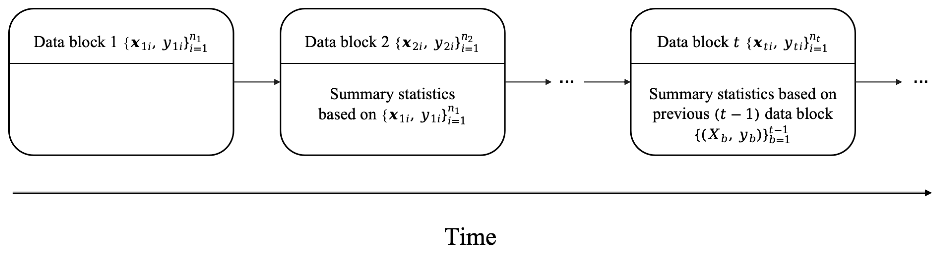
Figure 2.
Check function .
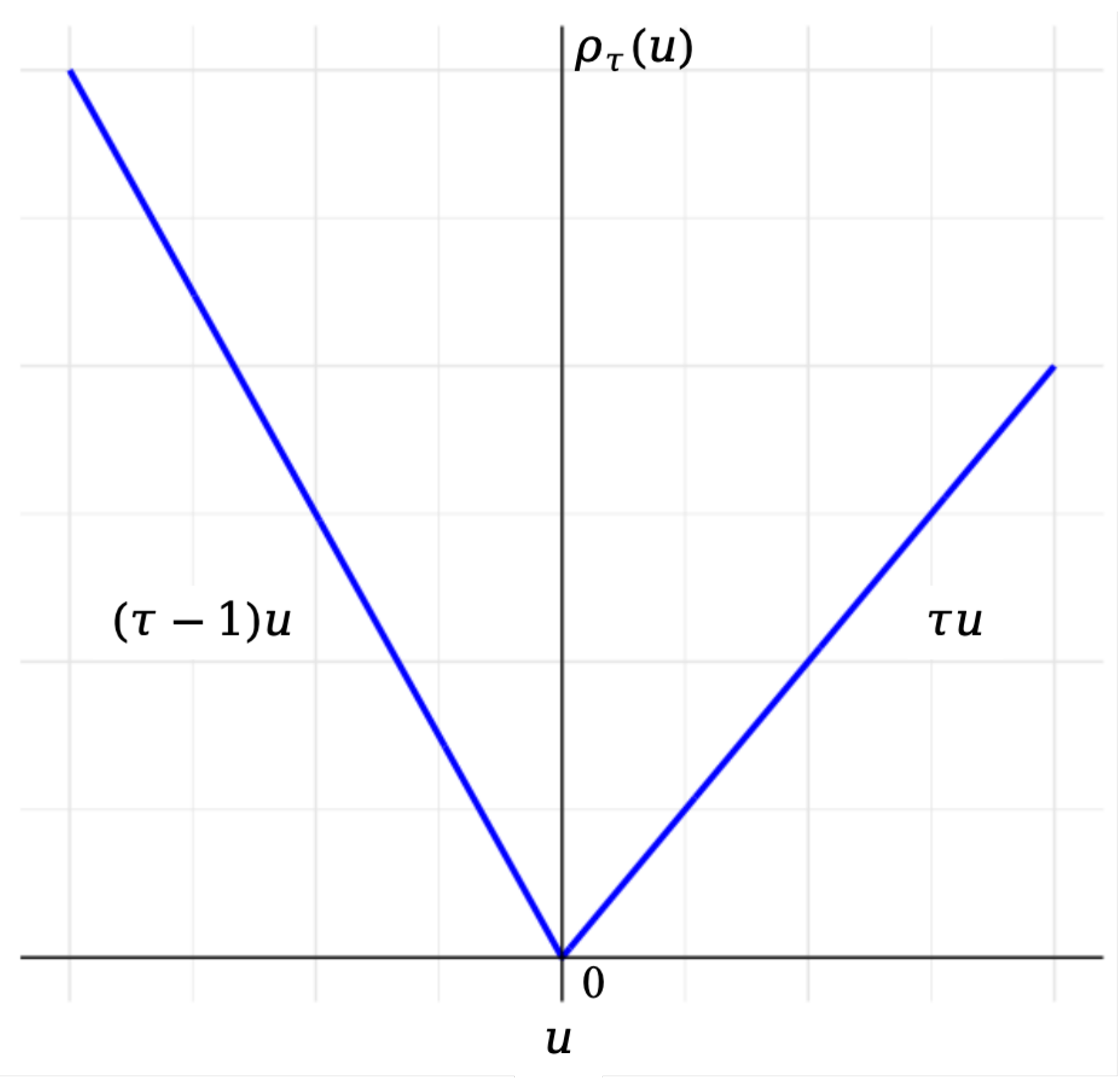
Figure 3.
Brief summarize of common estimation techniques for QR.
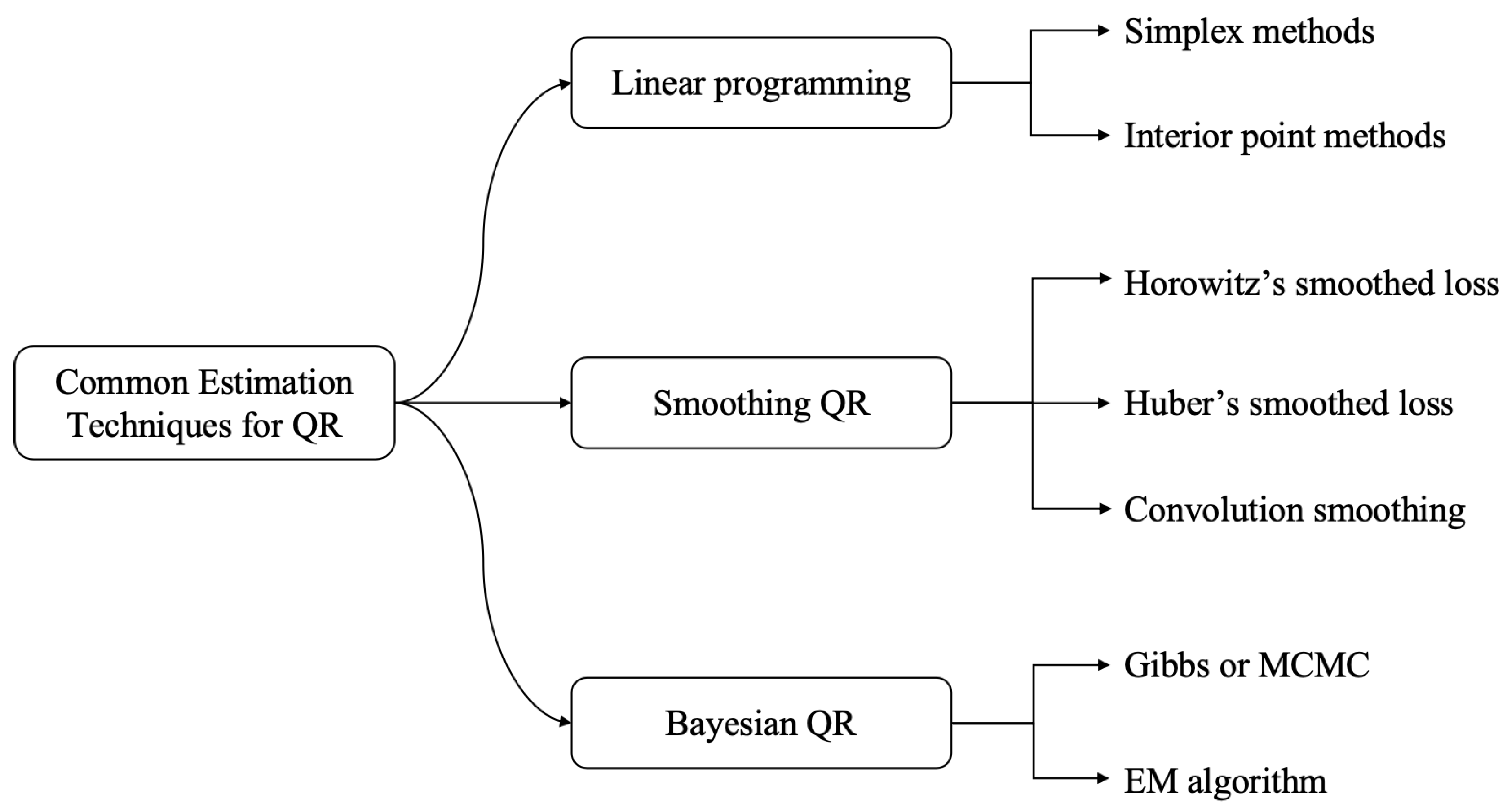
Figure 4.
Framework of dc algorithm.
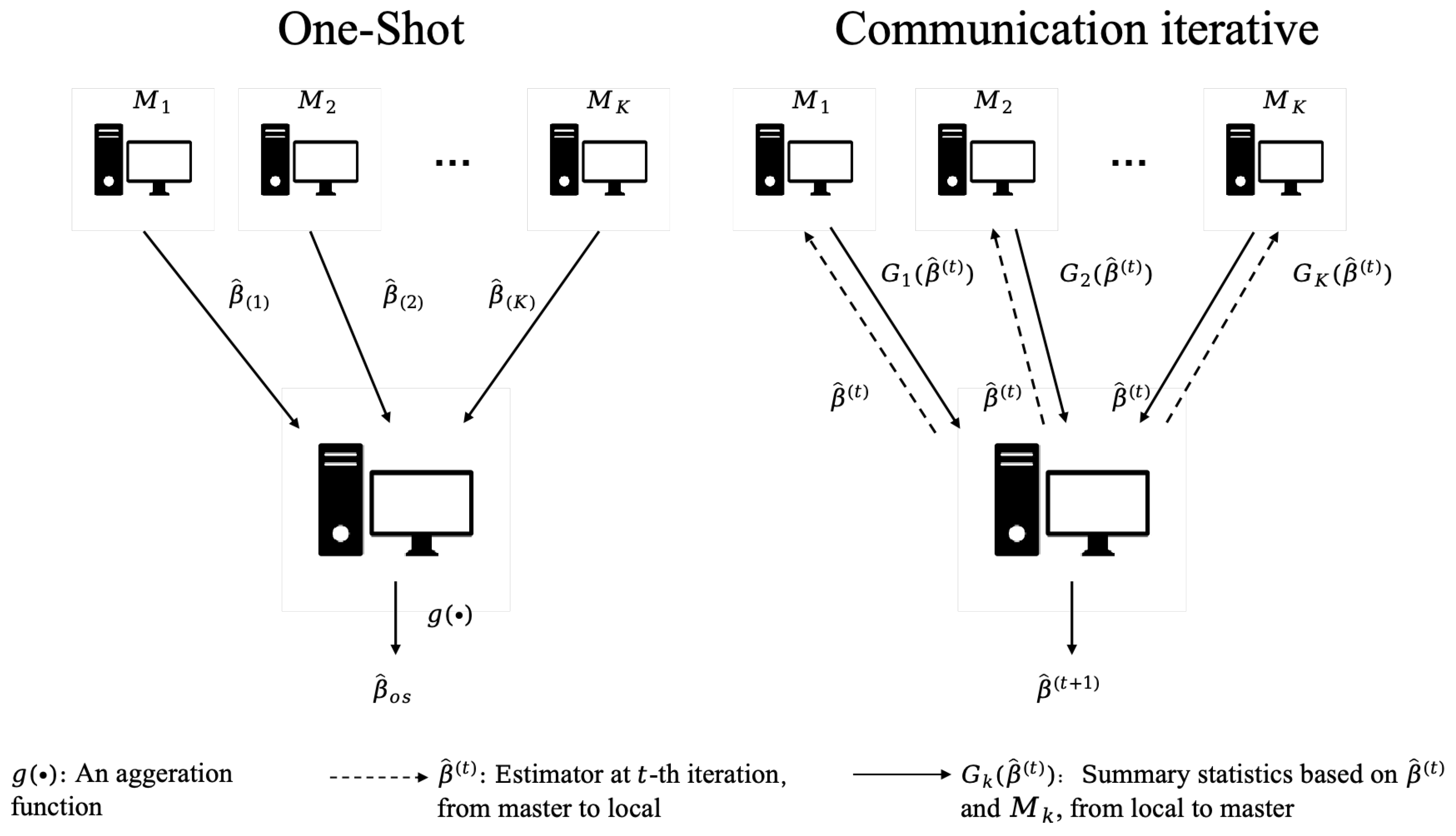

Table 1.
A brief summary of QR for large-scale data.
| Large-scale data | Data storage | Methodology | Brief Description |
|---|---|---|---|
| Massive data | Distributed storage | One-shot | Calculate estimator on each local machine using the data stored locally in a fully parallel manner. Subsequently, transmit the local estimator to a central machine, where they are combined to form the final estimator. |
| Iterative | Calculate some statistics on each local machine with local data. Transmit them to the central machine to update the global estimator and repeat the process until converge. | ||
| Stored on a single machine but too large to be fully loaded into the computer’s memory at once. | Subsampling | Repeatedly generate subsamples of small sizes for parameter estimation. | |
| Streaming data | Summary statistics based on historical data and the current data | Renewable | The resulting estimator is renewed with current data and summary statistics of historical data, without access to the historical data. |
Table 2.
A brief summary of quantile regression for massive data.
| Methology | Applicable Scene | Merit & Drawback |
|---|---|---|
| One shot | · Distributed across multiple nodes · Require low computation cost · Uniform distribution, with minimal heterogeneity between batches |
· High communication efficiency, simple to implement · Sensitive to data heterogeneity, accuracy may be limited |
| Iterative | · Distributed across multiple nodes · Require high estimation accuracy · Strong heterogeneity between batches |
· High accuracy, strong adaptability, theoretical guarantees · High communication cost, complex implementation |
| Subsampling | · Massive dataset, samples are sufficient to achieve a good estimate · Require low computation cost · Uniform data distribution or representative samples are available |
· High computational efficiency, simple to implement · Sensitive to data distribution, high randomness |
Table 3.
Brief summary of renewable algorithm for QR.
| Methodology | Form of solution | Brief Description |
|---|---|---|
| os-dc and its variants [7,11,23,41] | Close-form | Viewing stream data as data blocks partitioned over the time domain, only the estimate or summary statistics of each block are retained, and obtain the renewable estimation by aggregating the above statistics of each block. |
| sqr algorithm [12,90] | Iterative | Motivated by Bayesian QR, sequential updates occur naturally under the Bayesian setup, i.e., using the posterior distribution obtained from the past analysis as the prior information for later analysis. |
| cee-taylor-based [91,92,93,94,95] | Iterative | Reformulate the loss function using a Taylor expansion and apply the Newton algorithm for estimation, incorporating various smoothing techniques. |
Disclaimer/Publisher’s Note: The statements, opinions and data contained in all publications are solely those of the individual author(s) and contributor(s) and not of MDPI and/or the editor(s). MDPI and/or the editor(s) disclaim responsibility for any injury to people or property resulting from any ideas, methods, instructions or products referred to in the content. |
© 2025 by the authors. Licensee MDPI, Basel, Switzerland. This article is an open access article distributed under the terms and conditions of the Creative Commons Attribution (CC BY) license (http://creativecommons.org/licenses/by/4.0/).
Copyright: This open access article is published under a Creative Commons CC BY 4.0 license, which permit the free download, distribution, and reuse, provided that the author and preprint are cited in any reuse.


