1. Introduction
Accurate classification of mass spectrometry (MS)[
1] data is crucial for advances in environmental science[
2,
3],metabolomics[
4,
5], proteomics[
6], and medical diagnostics[
7,
8,
9]. However, MS data presents several challenges for machine learning (ML) algorithms, including high dimensionality[
10], complex feature distributions, batch effects[
11,
12,
13], and intensity discrepancies[
14]. These challenges often hinder model generalization[
15,
16,
17] and efficiency[
18,
19,
20], limiting their applicability to diverse datasets[
21].
Traditional ML methods, such as Random Forest [
22] and XGBoost [
23], have shown robust performance in high-dimensional data classification tasks [
24,
25]. However, they often require extensive feature engineering [
26,
27,
28], which can lead to information loss [
29] and may necessitate specialized biological expertise [
30]. Feature engineering, including feature selection [
31,
32,
33] and dimensionality reduction [
34], may filter out many low-abundance ions or unannotated m/z features, potentially impacting novel biomarker discovery or low-abundance protein identification in untargeted metabolomics or data-dependent proteomics studies [
35]. While deep learning models, particularly convolutional neural networks (CNNs), can handle high-dimensional data [
36,
37], they may struggle with generalization on small or imbalanced datasets [
38] common in MS analysis [
39,
40,
41].
The efficiency of an ML model is crucial for its practical application, particularly with large datasets or limited resources. Efficient models reduce computational demands, enabling faster training and inference, essential for time-sensitive MS-based applications like clinical diagnostics or real-time process monitoring. Furthermore, such models enhance accessibility by facilitating deployment on portable devices or within resource-constrained environments.
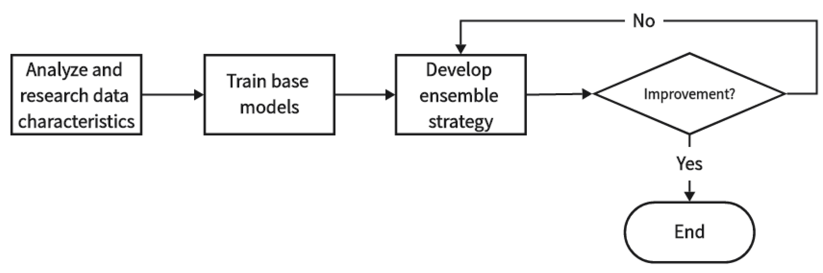
To address these challenges, this study introduces the Efficient Quick 1D Lite CNN Ensemble Classifier (EQLC-EC), an ensemble learning model for accurate and efficient classification of one-dimensional MS data. EQLC-EC integrates 1D convolutional networks with reshape layers and dual voting mechanisms to improve feature representation and classification performance. This approach aims to achieve high accuracy, computational efficiency, and robust generalization across diverse MS datasets.
This paper is structured as follows:
Section 2 reviews MS data analysis and related work, including challenges and existing methods.
Section 3 defines the problem statement and the MS data classification task.
Section 4 details the EQLC-EC architecture and methodology, encompassing the base classifier design and ensemble strategy.
Section 5 presents the experimental setup, datasets, and evaluation results of EQLC-EC compared to other methods.
Section 6 discusses the findings, analyzes EQLC-EC's performance, and explores future research directions. Finally,
Section 7 concludes by summarizing the key contributions and implications.
2. Basic Concepts and Research Status
This section introduces the fundamental concepts relevant to this research, providing the reader with a deeper understanding of the study.
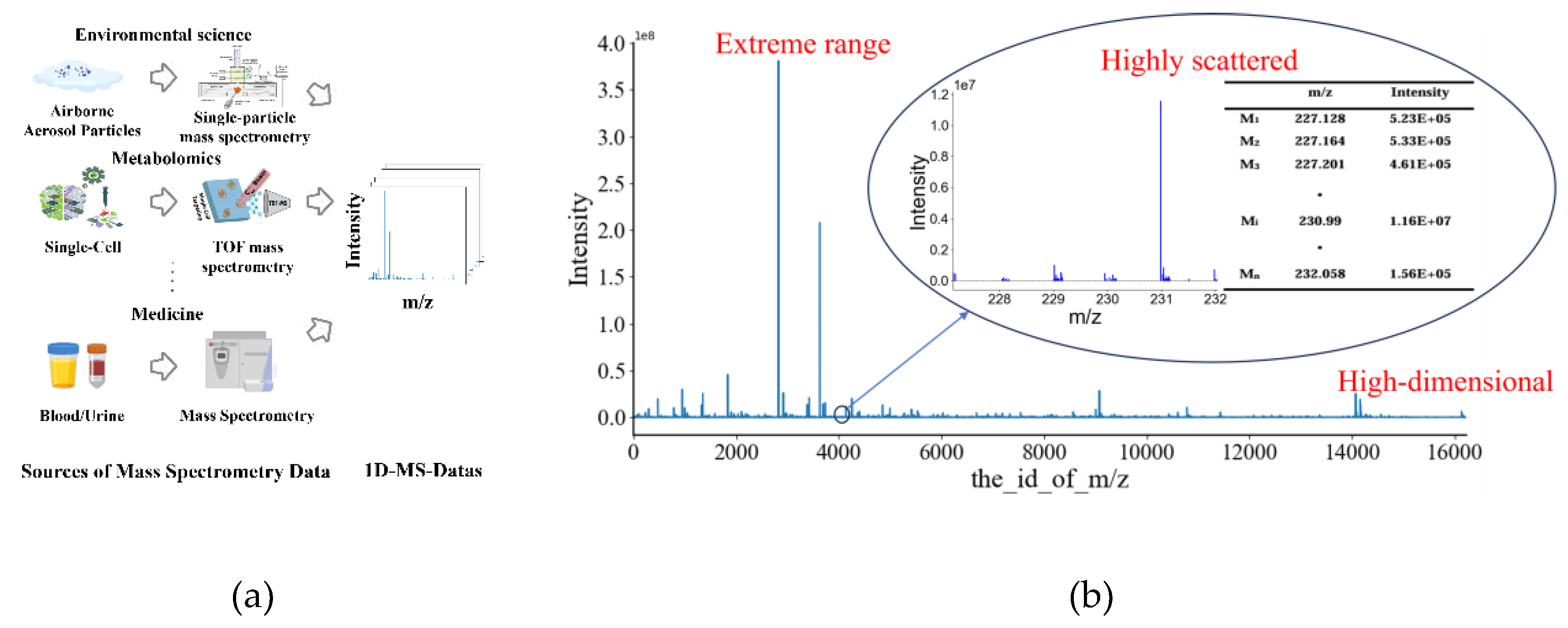
2.1. Mass Spectrometry and One-Dimensional Mass Spectrometry Data
Mass spectrometry (MS) [
1] is a powerful analytical technique used to identify different molecules present in a sample by measuring the mass-to-charge ratio of ions. In a typical MS workflow (
Figure 1a), molecules within a sample are first ionized. These ions are then separated and detected according to their mass-to-charge ratios [
42]. The information obtained is presented in the form of a mass spectrum, which is a plot of ion abundance versus mass-to-charge ratio.
One-dimensional mass spectrometry data refers to the most common form of this mass spectrum, where the x-axis represents the mass-to-charge ratio (m/z) of the ions and the y-axis represents the corresponding ion abundance (
Figure 1b). Therefore, one-dimensional mass spectrometry data is essentially a high-dimensional vector, where each dimension represents a specific m/z value, and its corresponding value represents the intensity of the ion at that m/z. This data contains a wealth of molecular information that can be used for various applications, including compound identification, protein structure studies, and disease diagnosis. However, one-dimensional mass spectrometry data also presents challenges for data analysis due to its high dimensionality, data sparsity, and large range of intensity values (
Figure 1b). These challenges have motivated the development of various data processing and analysis techniques, including the application of machine learning algorithms.
2.2. Machine Learning (ML) in MS
Machine learning (ML) [
43,
44,
45,
46,
47] has emerged as a powerful tool for analyzing mass spectrometry (MS) data, enabling the automated classification, identification, and quantification of molecules. ML algorithms can learn complex patterns and relationships within mass spectra, leading to improved accuracy and efficiency in data analysis. Various ML approaches have been applied to MS data, including supervised, unsupervised, and deep learning.
2.3. Challenges in Applying ML to MS Data
Despite the potential of ML in MS, several challenges hinder its widespread application and effectiveness:
High Dimensionality: MS data typically contain a large number of features (m/z values), often exceeding the number of samples. This high dimensionality can lead to overfitting[
48], where the ML model learns the training data too well and fails to generalize to unseen data.
Batch Effects: Systematic variations in data acquisition across different batches can introduce biases and confound the analysis. These batch effects can arise from differences in sample preparation, instrument settings, or experimental conditions.
Data Imbalance and Peak Intensity Polarization: The intensity values in MS data often exhibit an imbalanced distribution, with a wide dynamic range. This can lead to "peak intensity polarization," where the signals from low-abundance but potentially important compounds are obscured by the dominant signals from high-abundance compounds.
Generalization: The ability of an ML model to perform well on unseen data is crucial for its reliability and applicability. However, models trained on a single MS dataset often struggle to generalize to other datasets due to variations in data characteristics and experimental conditions.
2.4. Machine Learning Methods for MS Data
2.4.1. Traditional Machine Learning Methods
Traditional ML algorithms, such as Random Forest and XGBoost, have been widely used for MS data classification. These algorithms are particularly effective for handling high-dimensional data and can achieve robust performance. However, they often require feature engineering to reduce the computational burden and improve accuracy. Feature engineering involves selecting or transforming features to enhance the performance of the ML model. This process can be time-consuming and may lead to the loss of important information.
2.4.2. Deep Learning Methods
Deep learning (DL) models, particularly convolutional neural networks (CNNs), have shown promising results in MS data analysis. CNNs can automatically learn hierarchical feature representations from raw MS data, eliminating the need for manual feature engineering. This capability makes them well-suited for handling high-dimensional MS data and capturing complex patterns. However, DL models generally require large datasets for training and can be prone to overfitting when applied to small or imbalanced datasets.
2.5. Ensemble Learning
Ensemble learning combines multiple individual models to improve overall performance and generalization ability. By aggregating the predictions of multiple models, ensemble learning can reduce the risk of overfitting and enhance robustness. Different ensemble methods, such as bagging, boosting, and stacking, have been applied to MS data analysis with varying degrees of success.
2.6. Related Work And Recent Advances
2.6.1. Predominance of Traditional Machine Learning Methods in Review Papers
The application of machine learning for MS data classification is most prevalent in the field of disease diagnostics. A recent review on cancer diagnostics [
49] provides numerous examples of machine learning applications for early cancer detection. In a case-control study for early breast cancer diagnosis, Huang et al. [
50] analyzed plasma samples from early-stage and all-stage cancer patients to develop a series of predictive models, including SVM, RF, and LR, for breast cancer detection. In a study on triple-negative breast cancer detection [
51], Xiao et al. utilized a refined breast tissue metabolomics dataset and employed supervised learning to obtain predictive models, such as linear SVM and Least Absolute Shrinkage and Selection Operator (Lasso) regression, to compare their performance. In another study focusing on the detection of breast cancer estrogen receptor (ER) status [
52], a supervised deep learning (DL) approach was implemented using a feedforward artificial neural network (ANN) with input, output, and multiple hidden layers. Robust predictive models for liver cancer detection can be compiled through supervised ML algorithms, such as linear SVM [
53].
In a recent review on thyroid diseases [
54], Kumari et al. (2024) used age, gender, and hormone levels as features and combined them with three ML models to classify hyperthyroidism and hypothyroidism. The results indicated that XGBoost was the best-performing model for this task [
55]. Xi et al. (2022) constructed six ML models to predict the malignancy of thyroid nodules. RF and Gradient Boosting Machine (GBM) demonstrated better overall diagnostic accuracy and the ability to identify malignant nodules [
56]. Their approach can be used as additional evidence for the preoperative diagnosis of thyroid cancer. Guo et al. (2022b) built a diagnostic model for benign and malignant thyroid tumors. The benign group included five thyroid diseases, while the malignant group included six. Using clinical factors as features, RF, XGBoost, LightGBM, and AdaBoost models were constructed [
57]. The RF model exhibited the best performance.
A recent review in the field of food safety [
58] highlighted the application of machine learning algorithms, including Random Forest and Support Vector Machine, to improve food metabolomics classification and prediction tasks.
Another recent review encompassing food, pharmacology, environmental science, and forensic science [
59] indicated that the most commonly used methods for GC-MS data analysis are three ML algorithms [
60]: Random Forest (RF), Support Vector Machine (SVM), and Partial Least Squares Discriminant Analysis (PLS-DA). A review paper on mass spectrometry imaging [
61] mentioned that Random Forest, Logistic Regression, XGBoost, and Support Vector Machine are the most commonly used methods for classification tasks in supervised machine learning.
Regarding commonly used algorithms, in the field of machine learning for antibiotic resistance prediction using mass spectrometry data, over 15 different algorithms have been tested. Most studies applied more than one algorithm at a time. Among the most frequently used algorithms, SVM was found to be the most common, followed by RF, which was used in 22 different articles. Finally, logistic regression was found in 12 studies. Additionally, concerning Artificial Neural Networks (ANN), seven studies were identified that applied them by using Supervised Neural Networks (SNN) or Multilayer Perceptron (MLP). Moreover, in terms of deep learning methods, only two studies implemented Convolutional Neural Networks (CNNs) [
62].
2.6.2. Unique Applications and Complex Networks in Deep Learning Classification Methods
Tang et al. proposed a novel self-attention deep learning model [
63] consisting of six fully connected layers, three convolutional layers, and three pooling layers, a novel self-attention model for protein mass spectrometry cancer classification based on cosine self-similarity.
Yang et al. proposed an ANN model for the rapid classification of coffee origins by combining mass spectrometry analysis of coffee aroma with deep learning [
64]. This model is a Multilayer Perceptron (MLP) with three hidden layers. Its input layer consists of 1760 neurons, each of the three hidden layers consists of 100 neurons, and the output layer consists of six neurons corresponding to the six geographical origins of the coffee samples.
Li et al. (2024) investigated AttnPep, a deep learning method for peptide identification in shotgun proteomics based on self-attention, which consists of three main modules: input embedding, self-attention, and a decoder composed of ResNet and fully connected (FC) layers [
65].
In practice, deep learning classification methods for mass spectrometry data are highly specialized for specific classification tasks, as illustrated by the reviewed works. In a review [
66], Neely (2023) summarized deep learning methods for proteomics. Until recently, each data type had a specific neural network layer architecture best suited for it [i.e., Convolutional Neural Networks (CNNs) were mainly used for images, while Recurrent Neural Networks (RNNs) were mainly used for natural language text sequences]. However, a new general-purpose layer architecture, the transformer, can handle any input and output data modality. In short, this is achieved by using an attention-based stacked dense layer architecture. Notably, state-of-the-art models typically use transformers almost exclusively, without relying on other concepts such as convolutional or recurrent layers. However, it is important to note that while deep learning is currently the dominant technique in machine learning, it may be somewhat excessive for certain prediction tasks. Many deep learning methods cannot demonstrate that the improvements brought by complex network structures have practical value in real-world applications, as evidenced by improved generalization and improved final results.
2.6.3. Ensemble Learning as a Method to Enhance Base Model Performance
For the study of ensemble models, Picache et al. (2020) directly demonstrated the experimental results of EN-based PI obtained using tree ensemble learning methods [
67]: XGBoost [
23], RF [
22], etc., for a quantitative comparison of tree ensemble learning methods for perfume identification using a portable electronic nose.
Zhang et al. (2023) integrated three different models—Logistic Regression (LR), Random Forest (RF), and Support Vector Machine—using a voting method for a plasma biomarker panel for major depressive disorder treatment using quantitative proteomics and ensemble learning algorithms [
68].
Wei et al. (2020) utilized majority voting (hard voting) for the non-destructive classification of soybean seed varieties through hyperspectral imaging and ensemble machine learning algorithms [
69].
Zhu et al. (2024) used a stacking strategy to improve the secondary classification of patients with methylmalonic acidemia using an ensemble method of fourteen different machine learning methods [
70].
Miller et al. used a stacking ensemble method with 19 base learners for lung cancer survival prediction and biomarker identification through ensemble machine learning analysis of tumor core biopsy metabolomics data [
71].
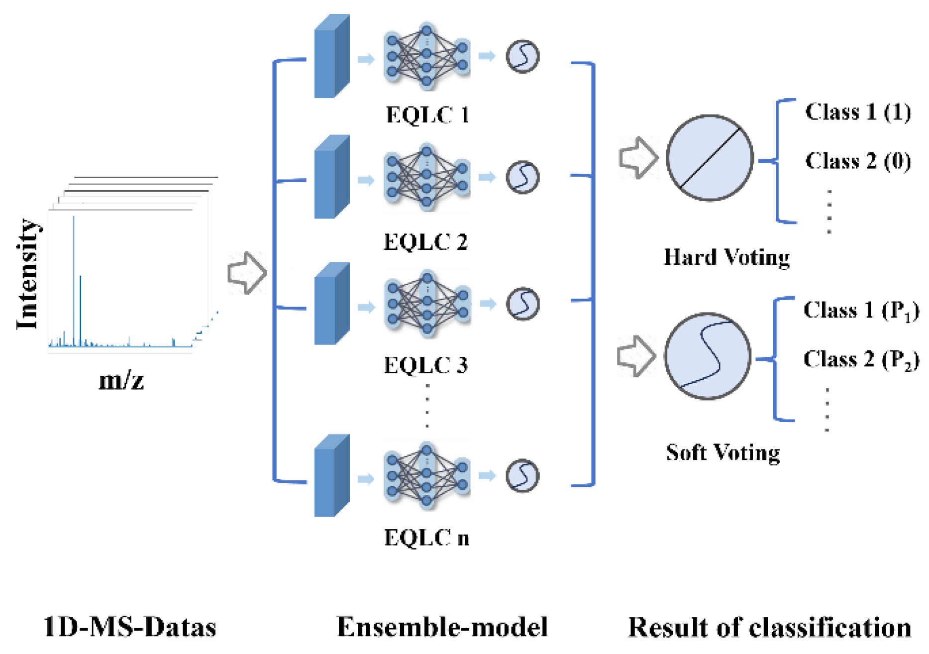
In fact, in the field of mass spectrometry, ensemble learning is more of a method to enhance the performance of base models. For example, Deng et al. utilized a voting method to enhance the performance of base models [
79]. The basic idea of the research is(
Figure 2):
3. Problem Statement and Task Description
The field of machine learning (ML) data classification faces several challenges:
Dataset and Task Specificity: Most research focuses on designing models for specific datasets and tasks, resulting in poor model generalization and difficulty in achieving good results on other datasets. Studies typically use only a single dataset for validation, lacking a generalized evaluation across multiple datasets[
72,
73].
Limitations of Traditional Methods: Traditional machine learning methods have high requirements for the quality of ML data and rely on tedious feature selection processes. Direct classification often results in low accuracy. Moreover, traditional methods rely on CPU computation, which is less efficient, especially when processing high-dimensional features, resulting in long computation times and limiting their application.
Resource Consumption of Deep Learning Methods: Deep learning methods leverage GPU parallel computing to improve efficiency, but complex network structures often require substantial computational resources, which may be lacking in many research institutions.
To address these challenges, this study aims to develop a versatile and lightweight model with the following objectives:
Lightweight Network Structure: Design a computationally efficient network structure to minimize resource consumption.
Enhanced Generalization Ability: Ensure that the model achieves good performance on multiple datasets of different types and conduct sufficient experimental validation.
4. Methodology
4.1. Dataset Description
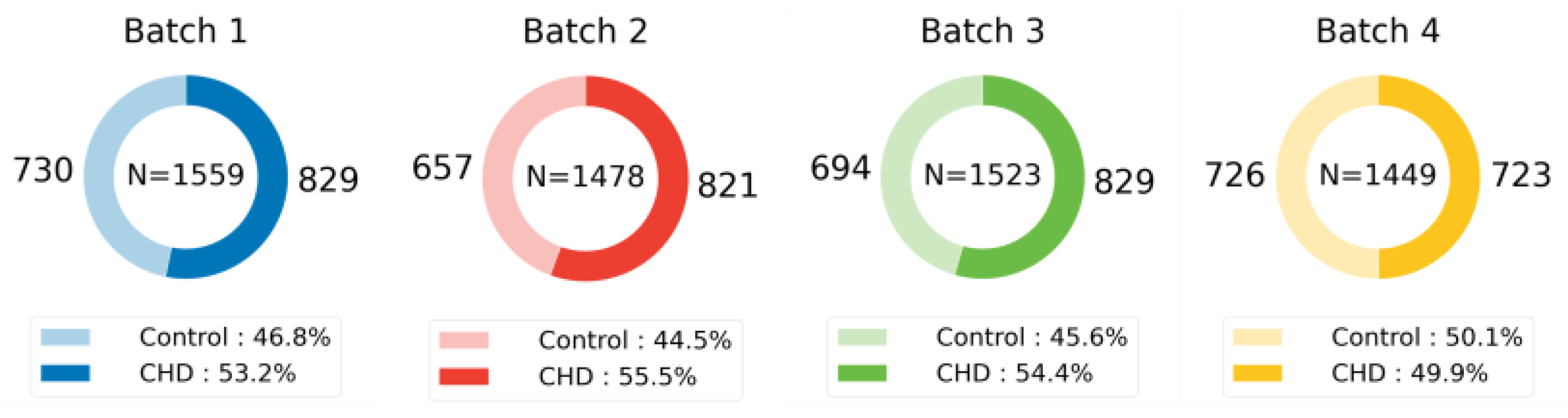
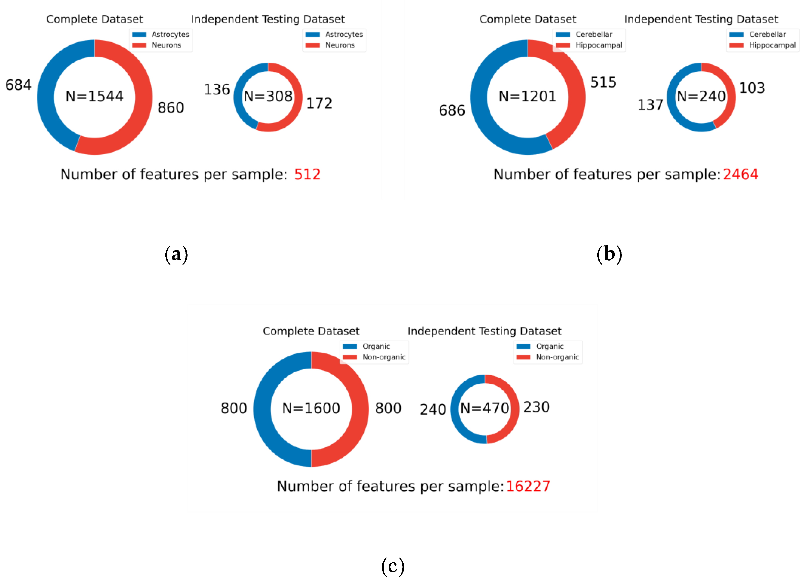
This study leverages five publicly available mass spectrometry datasets to rigorously evaluate the generalizability of machine learning models across a diverse range of domains. These datasets, summarized in
Table 1 and visualized in
Figure 3,
Figure 4 and
Figure 5, exhibit significant variations in their biological origins, sample sizes, and acquisition techniques, contributing to the breadth and depth of our analysis.
The deliberate inclusion of such diverse datasets is crucial for assessing the robustness and generalizability of machine learning models. By encompassing a wide spectrum of characteristics, these datasets provide a comprehensive platform to evaluate model performance under diverse conditions. This diversity manifests in several key aspects:
Biological Variability: The datasets represent a wide range of biological systems, from single cells (ICC and HIP_CER) and plant tissues (TOMATO) to human serum (MI and CHD). This diversity allows for the evaluation of model performance across different levels of biological organization and complexity.
Mass Spectrometry Platforms: The datasets were acquired using different instruments and ionization techniques, including MALDI-TOF, FT-ICR, and Orbitrap. This variation introduces differences in data acquisition, resolution, and potential biases, challenging the models to adapt to diverse data characteristics.
Data Structure and Preprocessing: Each dataset underwent specific preprocessing steps, including peak picking, alignment, and normalization. These variations in data handling further contribute to the diversity of the data landscape, requiring models to be robust to different preprocessing pipelines.
Furthermore, the sample distribution within each dataset plays a critical role in capturing the inherent diversity of the underlying biological phenomena. Visualized in
Figure 3,
Figure 4 and
Figure 5, the distribution of samples across different classes reflects the natural variability and prevalence of these classes in their respective domains. For example, the ICC dataset exhibits a relatively balanced distribution of neurons and astrocytes, while the MI and CHD datasets show varying degrees of class imbalance between control and disease groups. This diversity in sample distribution is essential for training models that can accurately represent and generalize across different populations and conditions.
By considering both the overall diversity of the datasets and the specific sample distributions within each dataset, we aim to provide a comprehensive and rigorous evaluation of machine learning models. This approach ensures that the models are not only accurate but also robust and generalizable to diverse real-world applications in various fields.
4.2. Data Preprocessing, Feature Extraction, and Splitting
This study utilizes preprocessed datasets with established feature selection, as provided by the original authors. Details of the preprocessing steps for each dataset can be found in the corresponding publications [
74,
77,
78]. To ensure consistency and comparability with existing state-of-the-art (SOTA) results, no additional data processing or feature selection was performed.
Dataset splitting strictly adhered to the ratios outlined in the original publications. In cases where only test set proportions and accuracies were reported without specific sample distributions, iterative random seed selection was employed to replicate performance closest to the published results. This process ensured the reproducibility and comparability of our results with existing benchmarks. The specific sample distributions and splitting details for each dataset are visualized in
Figure 3,
Figure 4 and
Figure 5.
Figure 3,
Figure 4 and
Figure 5 illustrates the sample distribution for each dataset, highlighting the prevalence of each class. This visualization provides insights into the composition of the training and test sets, showcasing the diversity in sample sizes and class representations across the datasets. Maintaining consistency in data splitting with the original studies ensures a fair comparison of model performance and facilitates the assessment of generalizability across different datasets and experimental conditions.
4.3. Model Training, Validation, and Evaluation
4.3.1. Experimental Setup
Model training, validation, and evaluation were conducted on a computer with the following specifications (
Table 2):
While the hardware configuration used in this study is not top-of-the-line server-grade, it represents a relatively high-performance setup for a personal computer. During the experiments, the model training did not approach the limits of the computational resources. Therefore, the experimental results exhibit a certain degree of generalizability and can serve as a reference for other researchers.
4.3.2. Lightweight Model Architectures
To identify the most computationally efficient approach for our classification task, we conducted a literature review of recent related work and selected five commonly used and state-of-the-art neural network architectures: MLP, 1DCNN, RNN, LSTM, and Transformer.
Given our focus on computational efficiency, we opted for simplified versions of each architecture to minimize computational overhead and ensure fair comparison. Specifically:
MLP: A simple multi-layer perceptron with two hidden layers, each with a size of 128 neurons.
1DCNN: A single-channel 1D convolutional neural network comprising two convolutional layers followed by two fully connected layers.
RNN: A recurrent neural network with a single recurrent layer and two fully connected layers. This simplified configuration facilitates direct comparison with the MLP model.
LSTM and Transformer: To further prioritize computational efficiency, both the LSTM and Transformer models were implemented with only a single fully connected layer for classification. This streamlined design reduces computational complexity while retaining the core functionalities of each architecture.
This deliberate emphasis on lightweight architectures stems from our objective to identify a model that not only achieves high accuracy but also minimizes computational demands, making it suitable for deployment in resource-constrained environments or real-time applications. Detailed network configurations and hyperparameter settings can be found in the git address provided in the Data Availability Statement.
4.3.3. Model Training
In this study, we adopted a consistent training strategy for all models, utilizing a fixed number of epochs with a decaying learning rate. This approach was motivated by our primary objective in this phase to obtain a preliminary understanding of the performance capabilities of each simplified network architecture. As such, extensive hyperparameter tuning was deemed unnecessary at this stage.
Specifically, all models were trained for 200 epochs. The learning rate was adjusted dynamically based on the observed convergence rate of each model on the training set, with a decay factor of 0.95 applied every 5 epochs. This learning rate scheduling strategy allows for a balance between rapid initial learning and fine-grained optimization in later stages of training.
This standardized training approach, while not necessarily yielding the absolute optimal performance for each individual model, ensures a fair and consistent comparison across different architectures. It allows us to focus on the inherent capabilities of each model under a unified training regime, facilitating a clear assessment of their relative computational efficiency and classification performance.
4.3.4. Model Performance Evaluation
Computational Efficiency Analysis: This study places a significant emphasis on computational efficiency. To comprehensively assess the performance of each model, we consider the following metrics: CPU Usage (%), GPU Memory Allocated (MB), GPU Memory Reserved (MB), Epoch Train Time (s), and Inference Time (s). These metrics provide insights into the resource utilization and processing speed of each model, allowing for a thorough evaluation of their computational efficiency.
Table 3.
Computational efficiency evaluation metrics.
Table 3.
Computational efficiency evaluation metrics.
| Metric |
Description |
| CPU Usage (%) |
CPU utilization. |
| GPU Memory Allocated (MB) |
The amount of GPU memory allocated to the model during training and inference |
| GPU Memory Reserved (MB) |
The amount of GPU memory reserved by the model during training and inference |
| Epoch Train Time (s) |
The average time taken to train the model for a single epoch |
| Inference Time (s) |
The average time taken by the model to generate a prediction on a single input sample |
Model Accuracy Analysis: To evaluate the classification performance of each model, we utilize several metrics:
Accuracy: The ratio of correctly classified samples to the total number of samples.
Precision: The ratio of correctly predicted positive observations to the total predicted positive observations.
Recall: The ratio of correctly predicted positive observations to all observations in the actual class.
F1-score: The weighted average of Precision and Recall.
While all the aforementioned metrics are recorded and analyzed, we primarily focus on accuracy and F1-score in the main text to enhance readability and conciseness.
Standard Deviation Analysis: To assess the stability and robustness of our models, we conduct standard deviation analysis. This involves training and evaluating the models on different batches of data within the development dataset. This analysis helps us understand the variability in model performance across different data subsets and provides insights into the generalization capabilities of each model.
4.4. Classifier Selection and Description
4.4.1. Selection of Base Classifiers
Our selection of classifiers was guided by two fundamental principles: versatility and accuracy.
Versatility: Our goal was to identify a classifier with broad applicability in mass spectrometry data analysis. This necessitates several key characteristics:
Minimal data preprocessing: The classifier should be able to handle raw MS data with minimal preprocessing, reducing the need for specialized expertise in MS data handling and making the approach accessible to a wider range of researchers. This requirement effectively excludes many traditional machine learning methods, focusing our attention on deep learning approaches.
Low computational demands: Considering the limited availability of high-performance computing resources, the classifier should be executable on readily available GPUs in standard PCs, necessitating simplified deep network architectures.
Accuracy: Our objective also includes achieving high classification accuracy. In this regard, deep learning models such as CNN, RNN, Transformer, and MLP are promising candidates due to their demonstrated capabilities in various classification tasks. The selected classifiers, namely CNN, RNN, Transformer, and MLP, represent prevalent and widely adopted architectures in the field of deep learning, as evidenced by our comprehensive literature review in the preceding sections. These architectures offer a balance between versatility and accuracy, aligning with the objectives of this study.
4.4.2. Enhancing Diversity of Base Models
After determining the type of base classifier through comparative experiments, we proceeded to enhance the diversity of the selected base model. Common approaches for diversity enhancement include perturbing data samples, input features, learning parameters, and output representations.
In our study, which focuses on one-dimensional MS data, datasets often have a limited number of samples. Although the datasets used in this research do not suffer from extremely small sample sizes, we aimed to avoid sample perturbation techniques to ensure the broader applicability of our model. Additionally, considering that MS data classification often involves subsequent feature importance analysis, we also avoided feature perturbation methods, as they can complicate the interpretation of feature importance. Therefore, we opted for parameter perturbation, a technique well-suited to our specific circumstances.
After selecting the base model type, we trained multiple diverse base models by varying learning parameters such as learning rate and random initialization methods. This approach introduces variations in the model's training process, leading to a diverse set of base models with potentially different strengths and weaknesses.
4.5. Ensemble Model Construction
Given the performance limitations of the individual 1D CNN base models, we employed an ensemble learning strategy to enhance overall performance. Among various ensemble methods, we opted for the voting ensemble strategy based on several considerations, particularly its unique advantages in our research context compared to other ensemble strategies such as Bagging, Boosting, and Stacking:
4.5.1. Suitability Analysis of Voting Strategy
Firstly, the voting strategy aligns perfectly with our research objective of maintaining computational efficiency. Our base models are already lightweight 1D CNNs, and voting ensemble does not introduce additional model complexity. In contrast, Boosting methods (e.g., AdaBoost, Gradient Boosting) typically require iterative model training and sample weight adjustments, which significantly increase training time. While Stacking is a powerful method, it requires training a meta-learner to combine the outputs of base models, which also increases computational burden and model complexity, deviating from our principle of minimizing resource consumption. Although Bagging is relatively simple, in our scenario, the base model structure is already sufficiently simple with limited diversity. Therefore, the variations introduced by Bagging through data resampling may not be substantial enough to yield significant performance improvements.
Secondly, the simplicity and effectiveness of the voting strategy make it an ideal choice for handling high-dimensional mass spectrometry data. For simple base models, the core advantage of the voting strategy lies in its "low requirement" for model diversity. Even with 1D CNN models with identical structures and only differing initializations, as in our case, the inherent randomness in the training process can still produce prediction results with certain variations. The voting mechanism effectively leverages this diversity by adhering to the "majority rule" principle, reducing the error rate of individual models and improving overall accuracy and robustness. This is particularly crucial for high-dimensional, noisy mass spectrometry data, where simple models often struggle to capture all the complex patterns and are susceptible to noise. The voting strategy can effectively mitigate this issue.
4.5.2. Hard Voting and Soft Voting
Voting strategies can be categorized into hard voting, soft voting, and weighted voting. Weighted voting requires an additional validation set for base model weight selection, which necessitates a large number of samples, a condition not met by most mass spectrometry datasets. Therefore, we ultimately chose hard voting and soft voting strategies:
Hard Voting: Hard voting is a straightforward ensemble learning combination strategy that tallies the prediction results of multiple models and selects the class with the most votes as the final prediction.
Formula Explanation:
: The final prediction result of the ensemble model.
: The j-th class.
: Represents the j (class) that maximizes the following expression.
: Summation over the prediction results of T base models.
: Represents the number of votes (usually 0 or 1) that the i-th base model predicts sample x as class j.
Formula Interpretation: The hard voting formula indicates that for a given sample x, the ensemble model counts the prediction results (classes) of each base model for that sample and selects the class with the most votes as the final prediction.
Soft Voting: Soft voting is an ensemble learning combination strategy that synthesizes the prediction results of multiple models by averaging the predicted probabilities of each model as the final prediction.
Explanation:
: The final probability that the ensemble model predicts sample x as class j.
T: The number of base models.
: The probability that the i-th base model predicts sample x as class j.
Formula Interpretation: For a given sample x and class j, soft voting sums the probabilities that each base model predicts x as , and then divides by the total number of base models T to obtain the final prediction probability
4.5.3. Ensemble Model Performance Evaluation
Computational Efficiency Evaluation
We evaluated the computational efficiency of the ensemble model using three datasets with progressively increasing computational demands (refer to
Figure 5). During model development, we had already verified the computational efficiency of simple deep networks. Therefore, in these three datasets, we compared the computational efficiency of the ensemble model with commonly used high-performing models: Random Forest, SVM, XGBoost, and AdaBoost. These widely adopted machine learning models serve as suitable benchmarks for assessing the computational efficiency of our proposed ensemble approach, as they represent established and efficient methods for classification tasks.
Enhancement in Accuracy and Stability of Base Models
To validate the generalization ability of the ensemble model, we conducted experiments on four datasets. For the MI dataset with three batches of data (as shown in
Figure 3,
Figure 4 and
Figure 5), we compared the accuracy and F1-score of the ensemble model and the current state-of-the-art (SOTA) model on each batch to evaluate the stability of the ensemble model across different data batches. In the remaining three datasets, we reconstructed the test set 100 times using the bootstrap method and compared the test results of the ensemble model and the current SOTA method for each dataset. We then generated box plots of the accuracy to assess the performance improvement of the ensemble model compared to the base models and measured the improvement in stability through the standard deviation of the accuracy.
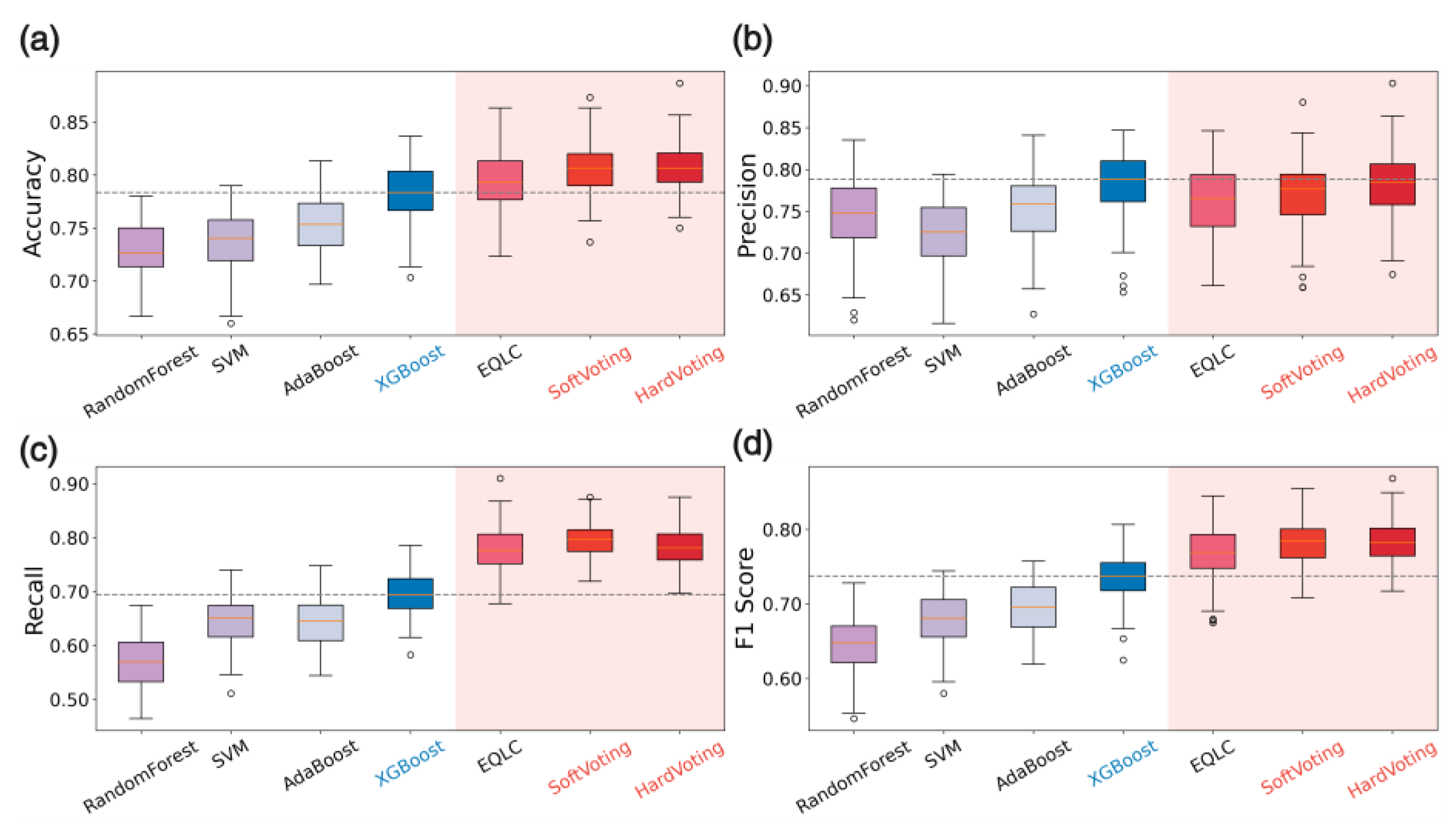
5. Results
This section presents the results of our study. We began by collecting and comparing five different publicly available, validated one-dimensional mass spectrometry datasets suitable for classification tasks. The CHD dataset was selected for model development due to its representative nature, large sample size, and availability of multiple batches, which allowed for comprehensive evaluation of model performance and generalizability. Through comparative experiments on simplified architectures of various deep learning models, the 1DCNN was identified as the most suitable base model due to its high accuracy and versatility. Subsequently, multiple EQLC models with the 1DCNN architecture were trained and ensembled using a voting strategy, resulting in the final EQLC-EC ensemble voting model. Our key findings are summarized as follows:
5.1. Evaluation of Computational Efficiency and Generalizability of Simplified Deep Learning Models
To evaluate the computational efficiency of different deep learning models, we analyzed simplified versions of five commonly used architectures: 1DCNN, LSTM, MLP, RNN, and Transformer. The simplified architectures were chosen to minimize computational overhead and ensure fair comparison. The impact of model complexity on performance is discussed in the Methodology section.
Table 4.
Computational efficiency and resource utilization of simplified deep learning networks.
Table 4.
Computational efficiency and resource utilization of simplified deep learning networks.
| Model |
CPUU
sage (%) |
GPU Memory
Allocated (MB) |
GPU Memory
Reserved (MB) |
Epoch Train
Time (s) |
Inference
Time (s) |
| Single_1DCNN |
3 |
23.59 |
256 |
0.05 |
0.04 |
| LSTM |
1.6 |
21.23 |
1738 |
0.10 |
0.02 |
| MLP |
4.3 |
17.28 |
24 |
0.03 |
0.03 |
| Single_RNN |
5.3 |
21.00 |
2258 |
0.14 |
0.03 |
| Transformer |
1.4 |
71.86 |
584 |
1.65 |
0.25 |
Analysis:
CPU Usage: The Single_RNN model exhibited the highest CPU usage (5.3%), followed by MLP (4.3%). Single_1DCNN (3%), LSTM (1.6%), and Transformer (1.4%) had relatively lower CPU usage. Overall, all five methods demonstrated low CPU utilization. Considering fluctuations due to background processes, these values can be considered very close.
GPU Memory: The Transformer model had the highest GPU memory allocation (71.86 MB) and usage (584 MB). LSTM and Single_RNN also exhibited high GPU memory usage, at 1738 MB and 2258 MB, respectively. Single_1DCNN and MLP had the lowest GPU memory usage.
Training Time: The Transformer model had the longest single-epoch training time (1.65 seconds), followed by Single_RNN (0.14 seconds) and LSTM (0.10 seconds). Single_1DCNN and MLP had the shortest training times, at 0.05 seconds and 0.03 seconds, respectively.
Inference Time: The Transformer model had the longest total inference time (0.25 seconds). The other models had shorter and more comparable inference times.
In terms of computational efficiency and resource utilization, all simplified networks demonstrated very low resource consumption. Standard GPUs with parallel computing capabilities are sufficient to meet the research requirements.
5.2. Superior Performance and Versatility of 1DCNN among Simplified Deep Networks
We evaluated the performance of five simplified neural network architectures—MLP, Single_1DCNN, Single_RNN, LSTM, and Transformer—on the CHD dataset. This dataset comprises four batches of data. For each test, two batches were combined to form the training set, while the remaining two batches were used as individual test sets. The accuracy and F1-score results are presented in
Table 5 and
Table 6, respectively.
Analysis of Accuracy: MLP (0.795) and Single_1DCNN (0.783) achieved the highest average accuracy on the CHD dataset, demonstrating the superior ability of MLP and CNN networks to discern features in one-dimensional mass spectrometry data. In contrast, Single_RNN (0.650), LSTM (0.584), and Transformer (0.560) showed relatively lower accuracy. In terms of stability, Transformer exhibited the smallest standard deviation (0.014), indicating consistent performance across different training/testing set combinations. Single_1DCNN also demonstrated good stability with a low standard deviation (0.024). MLP, Single_RNN, and LSTM had significantly higher standard deviations, suggesting greater variability in performance.
Analysis of F1-score: Single_1DCNN (0.799) and MLP (0.803) achieved the highest average F1-scores on the CHD dataset, further confirming their strong feature recognition capabilities. Single_RNN (0.663), LSTM (0.534), and Transformer (0.485) had lower F1-scores. Single_1DCNN demonstrated the best stability with the lowest standard deviation (0.024). Transformer, despite its low standard deviation in accuracy, showed higher variability in F1-score (0.048), indicating instability in precision and recall. MLP, Single_RNN, and LSTM also exhibited higher standard deviations compared to Single_1DCNN.
Conclusion: MLP achieved the highest accuracy and F1-score, with Single_1DCNN performing very closely. The other three methods showed lower accuracy. In terms of stability, Single_1DCNN demonstrated the best performance. Considering that this preliminary model validation was a qualitative process without rigorous hyperparameter tuning, we can conclude that MLP and 1DCNN exhibit comparable capabilities in discerning features from one-dimensional mass spectrometry data.
5.3. EQLC-EC Ensemble Model
5.3.1. Base Model EQLC with 1DCNN Architecture
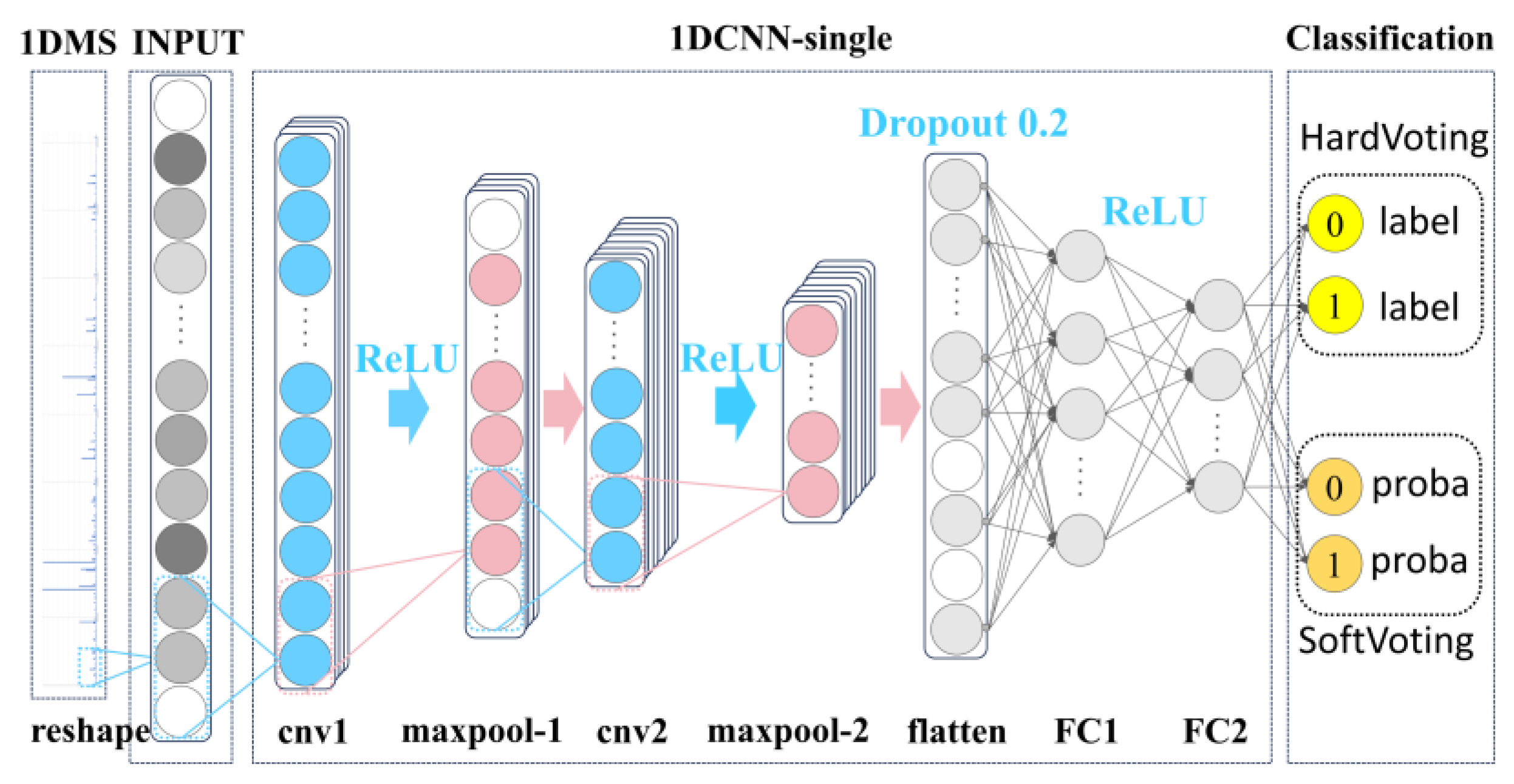
Based on the preceding analysis, we selected the 1DCNN as the network architecture for our base model, as illustrated in
Figure 6. EQLC Base Model:
Reshape Layer: Transforms raw input data into a uniform dimension, ensuring compatibility with subsequent network layers.
1DCNN-Single: The comparison with MLP demonstrated the minimal contribution of convolutional layers to classification accuracy. However, the convolutional layer plays a crucial role by representing m/z abundance in a transformed manner, thereby enhancing model stability and generalization ability across multiple batches. This layer also introduces diversity for different parameter settings of EQLC, which is essential for ensemble learning.
Classification Layer: Comprises a flattening layer and two fully connected layers for final classification. Outputs include classification labels for hard voting and probabilities for soft voting.
To ensure diversity, we created ten EQLC base models with varying parameters, as detailed in
Appendix A.
Table 7.
Test accuracy of the 10 base models.
Table 7.
Test accuracy of the 10 base models.
| Train-ing |
testing |
EQLC1 |
EQLC2 |
EQLC3 |
EQLC4 |
EQLC5 |
EQLC6 |
EQLC7 |
EQLC8 |
EQLC9 |
EQLC10 |
Sota by paper[65] |
| 1、2 |
3 |
0.785 |
0.763 |
0.763 |
0.785 |
0.783 |
0.784 |
0.760 |
0.768 |
0.782 |
0.779 |
0.739 |
| 1、2 |
4 |
0.744 |
0.756 |
0.767 |
0.747 |
0.770 |
0.735 |
0.754 |
0.758 |
0.735 |
0.767 |
0.744 |
| 1、3 |
2 |
0.777 |
0.788 |
0.784 |
0.787 |
0.785 |
0.779 |
0.794 |
0.784 |
0.792 |
0.783 |
0.794 |
| 1、3 |
4 |
0.785 |
0.793 |
0.794 |
0.794 |
0.797 |
0.785 |
0.785 |
0.799 |
0.792 |
0.798 |
0.732 |
| 1、4 |
2 |
0.797 |
0.790 |
0.803 |
0.792 |
0.785 |
0.796 |
0.790 |
0.800 |
0.791 |
0.784 |
0.829 |
| 1、4 |
3 |
0.802 |
0.785 |
0.787 |
0.793 |
0.801 |
0.800 |
0.785 |
0.786 |
0.795 |
0.797 |
0.779 |
| 2、3 |
1 |
0.826 |
0.829 |
0.828 |
0.836 |
0.838 |
0.822 |
0.831 |
0.822 |
0.837 |
0.844 |
0.793 |
| 2、3 |
4 |
0.815 |
0.796 |
0.799 |
0.810 |
0.812 |
0.812 |
0.796 |
0.799 |
0.813 |
0.818 |
0.761 |
| 2、4 |
1 |
0.815 |
0.803 |
0.816 |
0.823 |
0.827 |
0.807 |
0.802 |
0.815 |
0.819 |
0.827 |
0.865 |
| 2、4 |
3 |
0.810 |
0.797 |
0.788 |
0.797 |
0.798 |
0.808 |
0.793 |
0.786 |
0.797 |
0.793 |
0.807 |
| 3、4 |
1 |
0.800 |
0.795 |
0.816 |
0.806 |
0.810 |
0.795 |
0.790 |
0.810 |
0.805 |
0.808 |
0.817 |
| 3、4 |
2 |
0.765 |
0.750 |
0.786 |
0.780 |
0.769 |
0.766 |
0.746 |
0.777 |
0.781 |
0.759 |
0.822 |
| Average |
0.793 |
0.793 |
0.787 |
0.794 |
0.796 |
0.798 |
0.791 |
0.786 |
0.792 |
0.795 |
0.796 |
0.790 |
| Standard Deviation |
0.022 |
0.023 |
0.022 |
0.019 |
0.022 |
0.021 |
0.023 |
0.023 |
0.019 |
0.025 |
0.025 |
0.041 |
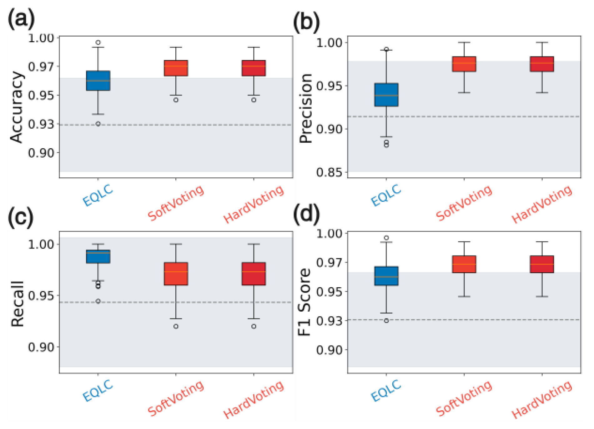
5.3.2. Dual Enhancement in Accuracy and Generalization Ability with Ensemble Model
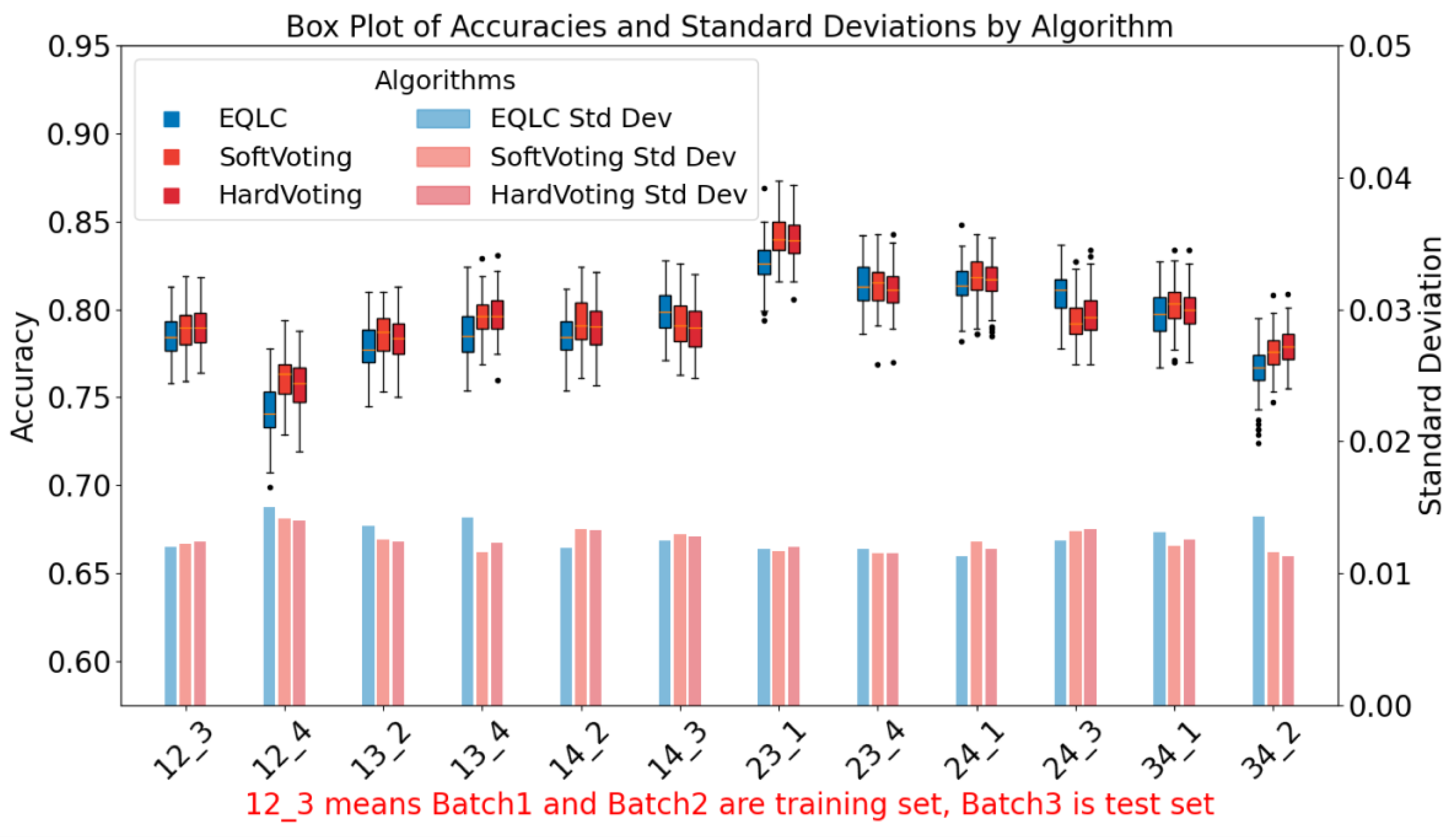
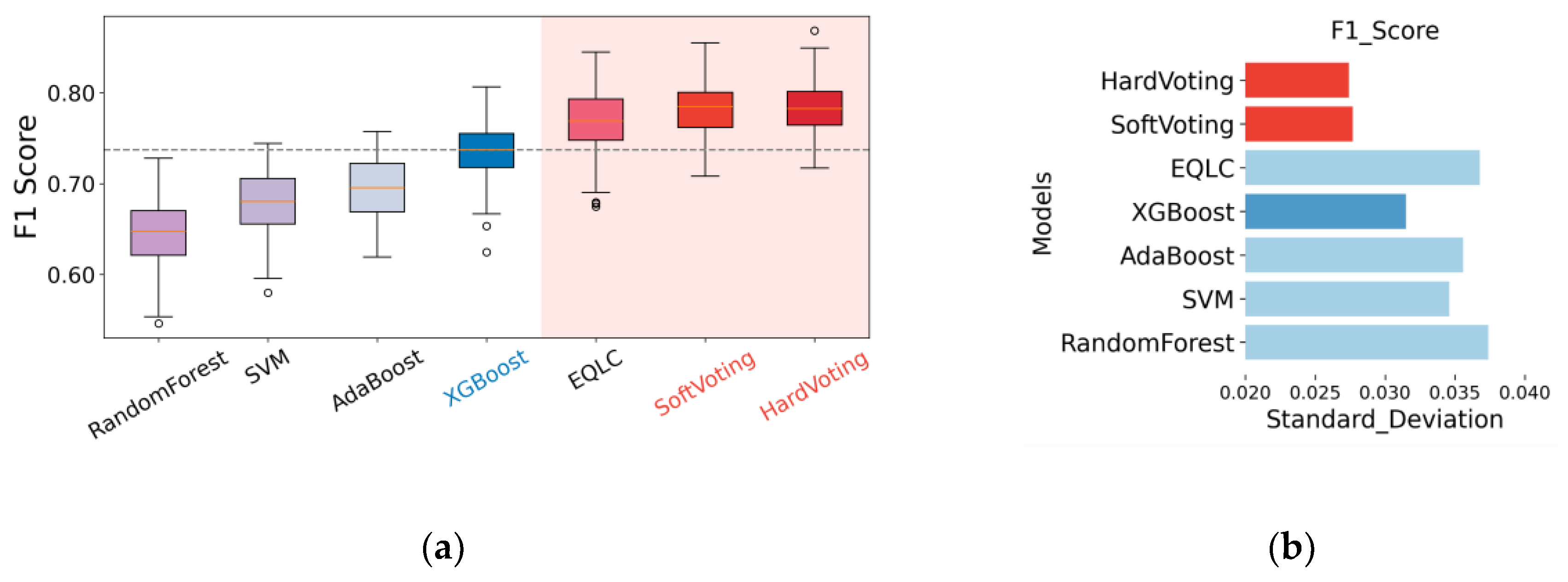
To thoroughly compare the stability of the base model EQLC and the ensemble model EQLC-EC, we conducted tests not only on different batches but also employed a bootstrap method to reconstruct the test set 100 times. This resulted in 100 test accuracy values for each test, which were then visualized as box plots, as shown in
Figure 8.
From the results in
Figure 8, we can conclude that both soft voting and hard voting methods of EQLC-EC demonstrate improvements in accuracy and stability compared to the base model EQLC:
Accuracy Improvement: In almost all cases (except 14_3, 24_3), the median of the box plots for soft voting and hard voting is higher than that of the EQLC model, indicating that the ensemble model achieves higher accuracy in most scenarios. In some cases (e.g., 14_2, 23_1), the accuracy of EQLC is even lower than the lower quartile of the ensemble model's box plot, further demonstrating the superiority of the ensemble model.
Stability Improvement: The box plots for soft voting and hard voting are generally shorter than those of the EQLC model, indicating less fluctuation in accuracy and higher stability. The EQLC model exhibits numerous outliers in certain cases (e.g., 34_2), suggesting its susceptibility to instability under certain conditions.
Comparison of the Two Voting Strategies: As depicted in the figure, the accuracy and stability of soft voting and hard voting are comparable, with no clear advantage of one over the other. In some cases, soft voting exhibits slightly higher accuracy than hard voting (e.g., 13_2), while the opposite is observed in other cases (e.g., 24_1). Overall, both voting strategies perform well, and the choice between them can be made based on the specific application.
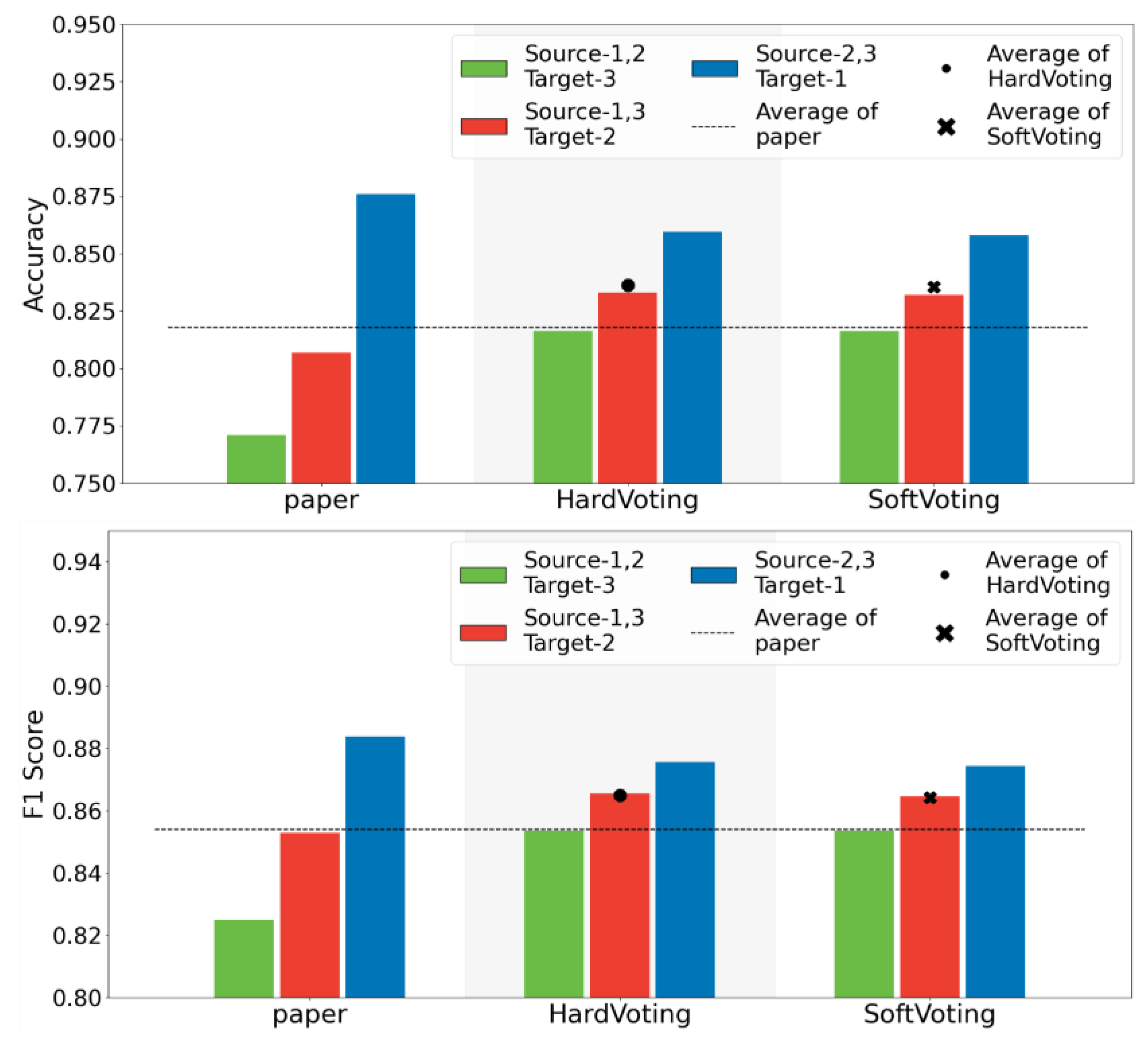
5.3.3. EQLC-EC Mitigates the Impact of Batch Effects
Having demonstrated the superior stability of the base model EQLC compared to other deep networks and the state-of-the-art (SOTA) method on the CHD development dataset, and further enhancement in stability with the ensemble model EQLC-EC, we sought to validate these findings on another dataset with multiple batches: the MI dataset. Due to differences in feature dimensions and specific m/z values compared to the development dataset, we retrained the model. The accuracy of the model and the test results of the SOTA method from the literature are shown in
Figure 9.
Stable Performance Across Different Data Splits: Observing the "Hard Voting" and "Soft Voting" bar graphs, we can see that regardless of the data split, the accuracy and F1-score of both voting strategies remain within a relatively stable range without significant fluctuations. This indicates that EQLC-EC is less susceptible to batch effects, maintaining good performance even when the training and test sets originate from different batches.
Superior Performance Compared to Single Models: Comparing the average performance (dots and crosses) of "Hard Voting" and "Soft Voting" with the original results from the "paper," we find that both voting strategies outperform the single model. This demonstrates that by ensembling multiple models, EQLC-EC can effectively mitigate the negative impact of batch effects and improve model generalization.
Comparison of the Two Voting Strategies: As shown in the figure, the performance of hard voting and soft voting is very close, with no clear advantage of one over the other. Under certain data splits, hard voting performs slightly better, while under others, soft voting shows superior performance.
Summary: Both voting strategies of EQLC-EC (hard voting and soft voting) effectively mitigate the impact of batch effects, improving model stability and generalization ability. The performance of the two strategies is similar, and the choice can be made based on the specific application.
5.3.4. High Computational Efficiency of EQLC-EC Validated Across Multiple Datasets
While ensemble models generally require more resources than base models, one of the key advantages of EQLC-EC is its low resource utilization. During base model selection, we prioritized models with minimal computational demands. To further validate the computational efficiency of EQLC-EC, we conducted experiments on three additional datasets from diverse domains. These datasets exhibit increasing computational scale due to variations in sample size and feature dimensions of the mass spectrometry data.
Analysis:
As shown in
Table 8, EQLC-EC consistently demonstrates superior computational efficiency compared to the other methods, particularly on the larger datasets. Notably, on the TOMATO dataset, EQLC-EC completed the experiment in approximately 1 hour and 10 minutes, while the other methods required significantly longer runtimes, ranging from 13 hours to 178 hours. This highlights the exceptional efficiency of EQLC-EC in handling high-dimensional mass spectrometry data.
The results underscore the effectiveness of our approach in minimizing computational demands while maintaining high accuracy and stability. EQLC-EC's low resource utilization makes it well-suited for deployment in various settings, including resource-constrained environments and real-time applications.
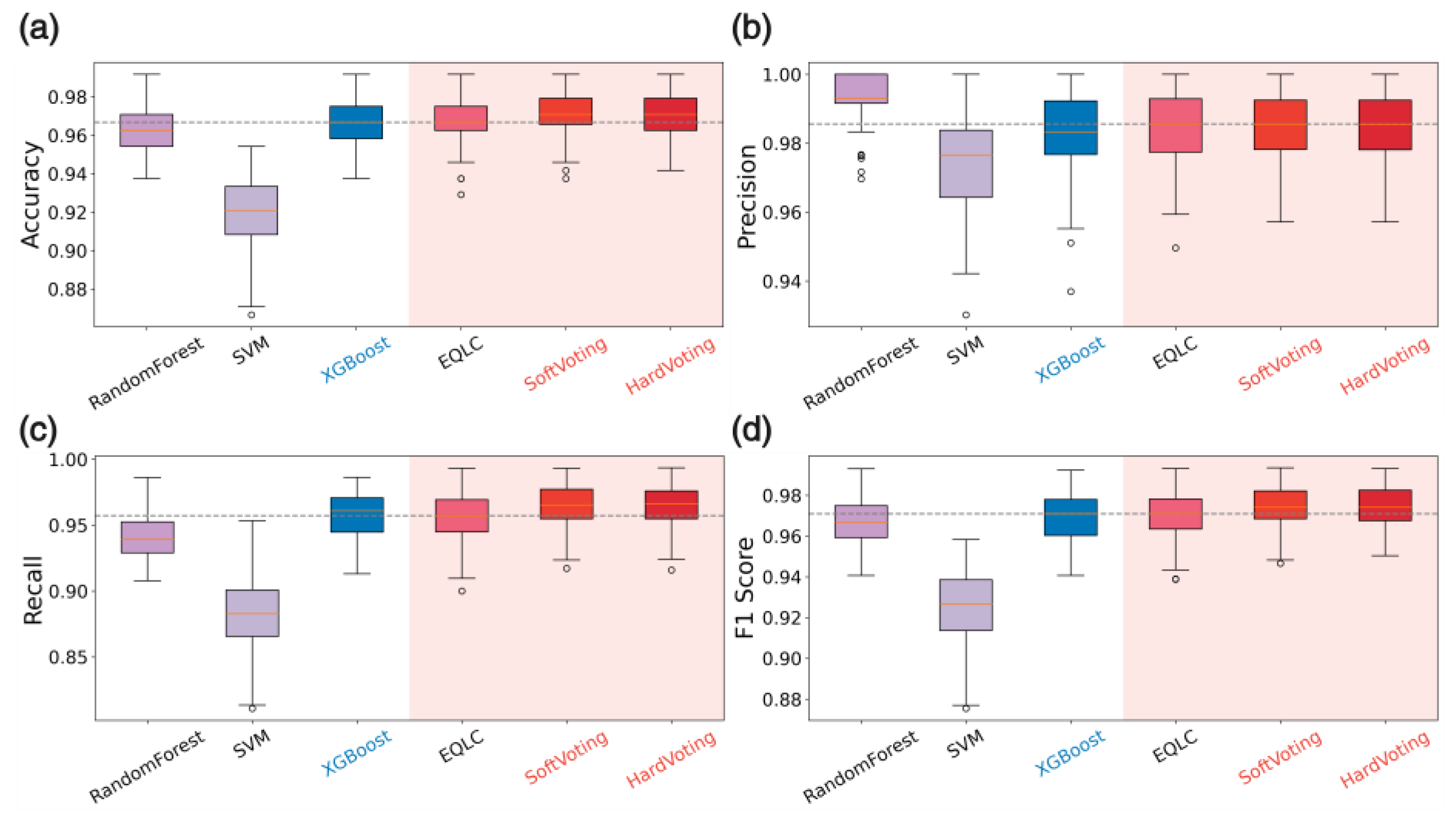
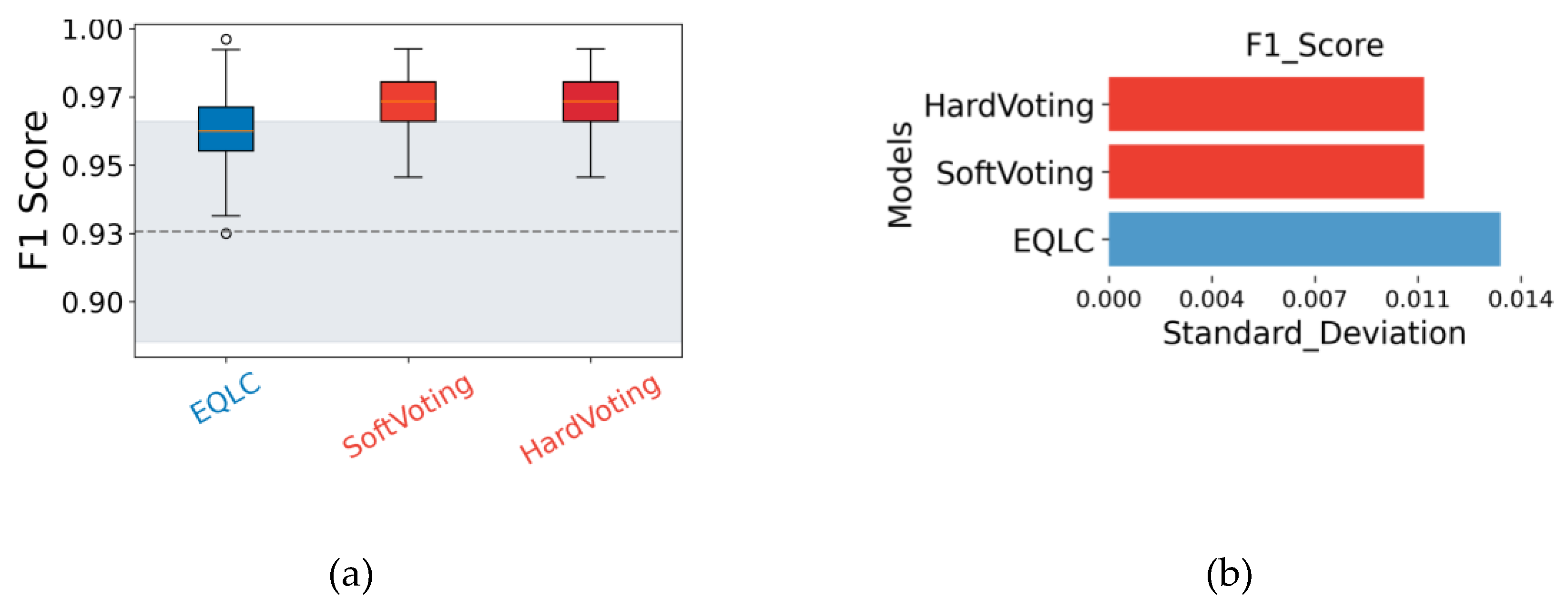
5.3.5. High Stability of EQLC-EC Validated Across Multiple Datasets
Developing an algorithm tailored to a single dataset does not necessarily demonstrate its generalizability and versatility. To assess the robustness of EQLC-EC, we evaluated its performance on multiple datasets. Considering the impracticality of excessively long experimental runtimes, we excluded methods with runtimes exceeding one day, as indicated by the blue markings in
Table 7. For conciseness, we present only the F1-score results in the main text (
Figure 10,
Figure 11 and
Figure 12), with results for other metrics available in
Appendix B (
Figure A1,
Figure A2 and
Figure A3).
Analysis:
The figures illustrate the consistent performance and high stability of EQLC-EC across multiple datasets. Specifically:
Superiority to SOTA methods: In
Figure 10a,
Figure 11a and
Figure 12a, EQLC-EC demonstrates comparable or superior F1-scores to the state-of-the-art (SOTA) XGBoost method on both the ICC and HIP datasets. Furthermore,
Figure 10b and
Figure 11b show that EQLC-EC exhibits lower standard deviations in F1-scores compared to XGBoost, indicating greater stability and robustness.
Improvement over the base model:
Figure 12 highlights the significant improvement in stability achieved by EQLC-EC compared to the EQLC base model on the TOMATO dataset. EQLC-EC consistently achieves higher F1-scores with lower standard deviations, demonstrating the effectiveness of the ensemble strategy in enhancing both accuracy and robustness.
These results underscore the effectiveness of EQLC-EC in achieving high performance with low computational cost and excellent stability across diverse mass spectrometry datasets.
6. Discussion
This study presents EQLC-EC, an ensemble deep learning model for the classification of one-dimensional mass spectrometry data. The model leverages the computational efficiency of GPUs and employs a simplified 1DCNN architecture to achieve high accuracy and stability with minimal resource consumption.
6.1. Deep Learning and Computational Efficiency
While deep learning often conjures images of powerful server farms and specialized hardware, this research demonstrates that substantial gains in computational efficiency can be achieved even with modest GPU resources. By leveraging the parallel processing capabilities of GPUs, even entry-level graphics cards can significantly accelerate training and inference times compared to traditional CPU-bound machine learning methods. This study highlights that the benefits of deep learning for mass spectrometry analysis are not limited to those with access to high-performance computing. Researchers with standard GPUs commonly found in today's workstations can readily utilize our proposed methods, opening new avenues for efficient and accessible data analysis.
This accessibility is particularly important for mass spectrometry, where datasets can be large and complex. Our findings show that simplified deep learning models, when implemented on GPUs, can efficiently handle these datasets, enabling faster turnaround times for research and analysis. This democratizes the use of deep learning in mass spectrometry, allowing a wider range of researchers to leverage its power for scientific discovery.
6.2. Simplified Architectures for High-Dimensional Data
This study challenges the prevailing notion that increasingly complex deep learning architectures are always superior. While models like Transformers have undeniably revolutionized fields like natural language processing, their success often hinges on two crucial factors: massive datasets and extensive hyperparameter tuning. These requirements pose a significant challenge for mass spectrometry data analysis, where datasets are often characterized by high dimensionality but limited sample sizes.
In this context, simpler architectures, such as the 1DCNN employed in this study, offer a compelling advantage. They require less data to train effectively, mitigating the risk of overfitting, a common pitfall when complex models are trained on small datasets. Overfitting occurs when a model learns the training data too well, capturing noise and outliers that hinder its ability to generalize to new, unseen data. Simplified models are inherently less prone to this issue.
Furthermore, simpler architectures require less hyperparameter tuning. Complex models with numerous layers and intricate connections often have a vast hyperparameter space, requiring extensive experimentation and computational resources to optimize. This process can be particularly challenging with limited data, as it becomes difficult to assess the true generalization ability of the model.
By adopting a simplified 1DCNN architecture, this study demonstrates that high accuracy and robust performance can be achieved in mass spectrometry analysis without the complexities and computational overhead associated with more elaborate models. This approach not only improves computational efficiency but also enhances the interpretability and reproducibility of the results, as the model's behavior is more easily understood and controlled.
6.3. CNNs for Local Feature Extraction
The superior performance of CNNs over RNNs and Transformers in this study suggests that local features play a more significant role in the classification of one-dimensional mass spectrometry data than temporal or sequential relationships. CNNs excel at capturing local patterns and spatial dependencies, which aligns with the observation that different m/z values in mass spectrometry data tend to exhibit a degree of independence in the time dimension.
6.4. Model Diversity and Ensemble Learning
Ensemble learning, which combines multiple models to improve accuracy and stability, relies on the diversity of its base models. This study demonstrates that even simple modifications to model hyperparameters can introduce sufficient diversity for effective ensemble learning. While further optimization could be achieved by selecting the most diverse models, this study prioritizes generalizability and applicability by including all trained models in the ensemble.
6.5. Voting Strategies for Ensemble Enhancement
This study employed both hard and soft voting strategies to leverage the strengths of the ensemble model. While both techniques enhanced performance, the nuances of each method and the reasons for employing both warrant further discussion.
Hard voting, also known as majority voting, operates on the principle of democracy. Each model in the ensemble casts a "vote" for the predicted class, and the class with the most votes wins. This approach is straightforward and computationally efficient, making it a popular choice for ensemble learning.
Soft voting, on the other hand, considers the probabilities assigned to each class by the individual models. It aggregates these probabilities, often by averaging, and the class with the highest combined probability is selected as the final prediction. This approach can be more nuanced than hard voting, as it takes into account the confidence levels of the individual models.
The choice between hard and soft voting often depends on the characteristics of the base models and the dataset. If the base models are diverse and tend to make different types of errors, hard voting can be effective in canceling out those errors. If the base models are well-calibrated and provide reliable probability estimates, soft voting can leverage those probabilities to make more informed predictions.
In this study, both hard and soft voting were implemented to explore the full potential of the ensemble model. The fact that neither method showed a clear advantage over the other suggests that both can be viable options for enhancing performance in mass spectrometry data analysis. The choice ultimately depends on the specific application and the preferences of the researcher.
Further investigation could delve into the conditions under which each voting method excels. For instance, analyzing the correlation between model predictions and the diversity of the ensemble could shed light on the scenarios where hard voting is most effective. Similarly, evaluating the calibration of the base models could provide guidance on when to favor soft voting. This deeper understanding would enable researchers to make more informed decisions about the most suitable voting strategy for their specific needs.
6.6. Generalizability and Future Directions
The strong performance of EQLC-EC across multiple datasets with diverse characteristics highlights its generalizability and robustness. The model's ability to handle variations in feature dimensions and data distributions underscores its potential for widespread application in mass spectrometry analysis. Future research could explore the interpretability of the model to gain deeper insights into the underlying features driving classification decisions.
7. Conclusions
This study introduces EQLC-EC, an ensemble deep learning model designed for efficient and accurate classification of one-dimensional mass spectrometry data. Key findings include:
Simplified architectures are effective: A streamlined 1DCNN architecture achieves high accuracy and stability, comparable to more complex models, while requiring less data and hyperparameter tuning. This makes it particularly well-suited for mass spectrometry data, which often has high dimensionality but limited sample sizes.
GPUs enhance efficiency: Leveraging the parallel processing power of GPUs, even those commonly found in standard workstations, significantly accelerates computation compared to traditional CPU-based methods. This makes deep learning analysis accessible to a wider range of researchers.
Ensemble learning improves robustness: Combining multiple 1DCNN models with varying hyperparameters into an ensemble enhances both accuracy and stability. Both hard and soft voting strategies prove effective for combining model predictions.
EQLC-EC generalizes well: The model demonstrates consistent performance across multiple datasets with diverse characteristics, outperforming existing state-of-the-art methods in several cases. This highlights its potential for broad application in various mass spectrometry analysis tasks.
EQLC-EC offers a compelling solution for mass spectrometry classification, combining accuracy, efficiency, and generalizability. By democratizing access to deep learning through its efficient design, EQLC-EC empowers researchers to extract valuable insights from complex mass spectrometry data.
Author Contributions
X.X. refers to Xingchuang Xiong. Conceptualization, X.X. and L.G.; methodology, L.G. and X.X.; software, L.G.; validation, Y.W., W.Z. and F.Z.; formal analysis, L.G.; investigation, L.G., Y.W., W.Z. and F.Z.; resources, X.X. and Z.L.; data curation, L.G.; writing—original draft preparation, L.G.; writing—review and editing, L.G. and X.X.; visualization, L.G.; supervision, X.X. and Z.L.; project administration, L.G.; funding acquisition, X.X. and Z.L. All authors have read and agreed to the published version of the manuscript.
Funding
This research was funded by Science & Technology Fundamental Resources Investigation Program, grant number 2022FY101200.
Data Availability Statement
All datasets referenced in this study are publicly available. The code associated with the proposed EQLC-EC model has been uploaded to
https://github.com/guolin247/EQLC-EC and is accessible for public use. Additionally, all raw data and preprocessed data files are included in the corresponding directories of the code repository, ensuring transparency and facilitating reproducibility testing.
Acknowledgments
The research at the National Institute of Metrology, China, has traditionally focused on metrology science, including extensive studies on mass spectrometry data. However, integrating these studies with computer science has been challenging. We extend our gratitude to the National Metrology Data Center for providing a research platform that enabled us to explore the integration of mass spectrometry techniques with computer science.
Conflicts of Interest
The authors declare no conflicts of interest. The funders had no role in the design of the study; in the collection, analyses, or interpretation of data; in the writing of the manuscript; or in the decision to publish the results.
Abbreviations
The following abbreviations are used in this manuscript:
| Acronyms |
Definitions |
| MS |
Mass spectrometry |
| ML |
Machine learning |
| EQLC-EC |
Efficient Quick 1D Lite CNN Ensemble Classifier |
| SVM |
Support vector machine |
| CNNs |
Convolutional neural networks |
| DL |
Deep learning |
| ANN |
Artificial neural network |
| LR |
Logistic Regression |
| Lasso |
Least Absolute Shrinkage and Selection Operator |
| SNN |
Supervised Neural Networks |
| ER |
Estrogen receptor |
| GBM |
Gradient Boosting Machine |
| RF |
Random Forest |
| PLS-DA |
Partial Least Squares Discriminant Analysis |
| MLP |
Multilayer Perceptron |
| GC-MS |
Gas chromatography-mass spectrometry |
| FT-ICR |
Fourier transform ion cyclotron resonance |
| MALDI-TOF |
Matrix-assisted laser desorption/ionization-time of flight |
| SOTA |
State-of-the-art |
| CHD |
Coronary heart disease |
| MI |
Myocardial infarction |
| ICC |
Cerebellar cells |
| HIP_CER |
Hippocampus and cerebellum cells |
Appendix A
Table A1.
Provides detailed parameters for all EQLC models in the EQLC-EC ensemble model corresponding to different datasets. The parameters include.
Table A1.
Provides detailed parameters for all EQLC models in the EQLC-EC ensemble model corresponding to different datasets. The parameters include.
Dataset Name
(Learning Rate Decay Strategy) |
Base model ID |
Learning rate |
Batch size |
Number of epochs |
Dropout value |
Random seed |
ICC
Learning rate decays by 0.95 every 30 epochs |
1 |
0.003 |
128 |
500 |
0.50 |
42 |
| 2 |
0.003 |
128 |
500 |
0.50 |
43 |
| 3 |
0.003 |
128 |
500 |
0.50 |
44 |
| 4 |
0.003 |
128 |
500 |
0.50 |
45 |
| 5 |
0.003 |
128 |
500 |
0.50 |
46 |
| 6 |
0.004 |
256 |
500 |
0.50 |
42 |
| 7 |
0.004 |
256 |
500 |
0.50 |
43 |
| 8 |
0.004 |
256 |
500 |
0.50 |
44 |
| 9 |
0.004 |
256 |
500 |
0.50 |
45 |
| 10 |
0.004 |
256 |
500 |
0.50 |
46 |
HIP_CER
Learning rate decays by 0.95 every 30 epochs |
1 |
0.001 |
256 |
400 |
0.00 |
42 |
| 2 |
0.001 |
256 |
400 |
0.00 |
45 |
| 3 |
0.001 |
256 |
400 |
0.00 |
46 |
| 4 |
0.001 |
256 |
1000 |
0.20 |
43 |
| 5 |
0.001 |
256 |
1000 |
0.20 |
46 |
| 6 |
0.001 |
256 |
1000 |
0.50 |
44 |
| 7 |
0.001 |
256 |
1000 |
0.50 |
46 |
TOMATO
Learning rate decays by 0.95 every 10 epochs |
1 |
0.00001 |
1024 |
50 |
0.20 |
42 |
| 2 |
0.00001 |
1024 |
50 |
0.20 |
43 |
| 3 |
0.00001 |
1024 |
50 |
0.20 |
44 |
| 4 |
0.00001 |
1024 |
50 |
0.20 |
45 |
| 5 |
0.00001 |
1024 |
50 |
0.20 |
46 |
| 6 |
0.00005 |
1024 |
50 |
0.20 |
42 |
| 7 |
0.00005 |
1024 |
50 |
0.20 |
43 |
| 8 |
0.00005 |
1024 |
50 |
0.20 |
44 |
| 9 |
0.00005 |
1024 |
50 |
0.20 |
45 |
| 10 |
0.00005 |
1024 |
50 |
0.20 |
46 |
MI
Learning rate decays by 0.98 every 30 epochs |
1 |
0.0002 |
128 |
2000 |
0.10 |
42 |
| 2 |
0.00015 |
64 |
2000 |
0.10 |
42 |
| 3 |
0.00015 |
64 |
2000 |
0.20 |
42 |
| 4 |
0.00015 |
64 |
2000 |
0.20 |
48 |
| 5 |
0.00015 |
64 |
2000 |
0.20 |
52 |
CHD*
Learning rate decays by 0.95 every 5 epochs |
1 |
0.00005 |
256 |
200 |
0.50 |
41 |
| 2 |
0.00005 |
256 |
200 |
0.50 |
42 |
| 3 |
0.00005 |
256 |
200 |
0.50 |
43 |
| 4 |
0.00005 |
256 |
200 |
0.50 |
44 |
| 5 |
0.00005 |
256 |
200 |
0.50 |
45 |
| 6 |
0.00006 |
256 |
200 |
0.50 |
41 |
| 7 |
0.00006 |
256 |
200 |
0.50 |
42 |
| 8 |
0.00006 |
256 |
200 |
0.50 |
43 |
| 9 |
0.00006 |
256 |
200 |
0.50 |
44 |
| 10 |
0.00006 |
256 |
200 |
0.50 |
45 |
Appendix B
Figure A1.
Performance comparison of EQLC-EC with other machine learning models on the ICC dataset. (a) Accuracy (b) Precision (c) Recall (d) F1-Score. The blue boxplot (XGBoost) represents the performance of the state-of-the-art method reported in the corresponding publication for this dataset.
Figure A1.
Performance comparison of EQLC-EC with other machine learning models on the ICC dataset. (a) Accuracy (b) Precision (c) Recall (d) F1-Score. The blue boxplot (XGBoost) represents the performance of the state-of-the-art method reported in the corresponding publication for this dataset.
Figure A2.
Performance comparison of EQLC-EC with other machine learning models on the HIP dataset. (a) Accuracy (b) Precision (c) Recall (d) F1-Score. The blue boxplot (XGBoost) represents the performance of the state-of-the-art method reported in the corresponding publication for this dataset.
Figure A2.
Performance comparison of EQLC-EC with other machine learning models on the HIP dataset. (a) Accuracy (b) Precision (c) Recall (d) F1-Score. The blue boxplot (XGBoost) represents the performance of the state-of-the-art method reported in the corresponding publication for this dataset.
Figure A3.
Performance comparison of EQLC-EC with other machine learning models on the TOMATO dataset. (a) Accuracy (b) Precision (c) Recall (d) F1-Score. The dashed line represents the average value of the state-of-the-art method reported in the corresponding publication, and the shaded area represents the confidence interval.
References
- Habler, K.; et al. Understanding isotopes, isomers, and isobars in mass spectrometry. J. Mass Spectrom. Adv. Clin. Lab. 2024, 33, 49–54. [Google Scholar] [CrossRef] [PubMed]
- Hildmann, S.; Hoffmann, T. Characterisation of atmospheric organic aerosols with one- and multidimensional liquid chromatography and mass spectrometry: State of the art and future perspectives. TrAC Trends Anal. Chem. 2024, 117698. [Google Scholar] [CrossRef]
- Gyftokostas, N.; et al. Laser-induced breakdown spectroscopy coupled with machine learning as a tool for olive oil authenticity and geographic discrimination. Sci. Rep. 2021, 11, 5360. [Google Scholar] [CrossRef] [PubMed]
- Barberis, E.; et al. Precision medicine approaches with metabolomics and artificial intelligence. Int. J. Mol. Sci. 2022, 23, 11269. [Google Scholar] [CrossRef] [PubMed]
- Galal, A.; Talal, M.; Moustafa, A. Applications of machine learning in metabolomics: Disease modeling and classification. Front. Genet. 2022, 13, 1017340. [Google Scholar] [CrossRef] [PubMed]
- Neely, B.A.; et al. Toward an integrated machine learning model of a proteomics experiment. J. Proteome Res. 2023, 22, 681–96. [Google Scholar] [CrossRef] [PubMed]
- Nilius, H.; et al. Machine learning applications in precision medicine: Overcoming challenges and unlocking potential. TrAC Trends Anal. Chem. 2024, 117872. [Google Scholar] [CrossRef]
- Shajari, E.; et al. Application of SWATH mass spectrometry and machine learning in the diagnosis of inflammatory bowel disease based on the stool proteome. Biomedicines 2024, 12, 333. [Google Scholar] [CrossRef] [PubMed]
- Harm, T.; et al. Machine learning insights into thrombo-ischemic risks and bleeding events through platelet lysophospholipids and acylcarnitine species. Sci. Rep. 2024, 14, 6089. [Google Scholar] [CrossRef] [PubMed]
- Clarke, R.; et al. The properties of high-dimensional data spaces: Implications for exploring gene and protein expression data. Nat. Rev. Cancer 2008, 8, 37–49. [Google Scholar] [CrossRef] [PubMed]
- Balluff, B.; et al. Batch effects in MALDI mass spectrometry imaging. J. Am. Soc. Mass Spectrom. 2021, 32, 628–35. [Google Scholar] [CrossRef] [PubMed]
- Yu, Y.; et al. Correcting batch effects in large-scale multiomics studies using a reference-material-based ratio method. Genome Biol. 2023, 24, 201. [Google Scholar] [CrossRef]
- Liu, Q.; et al. Addressing the batch effect issue for LC/MS metabolomics data in data preprocessing. Sci. Rep. 2020, 10, 13856. [Google Scholar] [CrossRef] [PubMed]
- Chen, G.; et al. MetTailor: Dynamic block summary and intensity normalization for robust analysis of mass spectrometry data in metabolomics. Bioinformatics 2015, 31, 3645–52. [Google Scholar] [CrossRef]
- Li, H.; et al. How does promoting the minority fraction affect generalization? A theoretical study of one-hidden-layer neural network on group imbalance. IEEE J. Sel. Top Signal Process. 2024; Epub ahead of print. [Google Scholar] [CrossRef]
- Wang, Y.; Patel, S.; Ortner, C. A theoretical case study of the generalization of machine-learned potentials. Comput. Methods Appl. Mech. Eng. 2024, 422, 116831. [Google Scholar] [CrossRef]
- Wiersch, L.; et al. Sex classification from functional brain connectivity: Generalization to multiple datasets. Hum. Brain Mapp. 2024, 45, e26683. [Google Scholar] [CrossRef]
- Barbiero, P.; Squillero, G.; Tonda, A. Modeling generalization in machine learning: A methodological and computational study. arXiv 2020, arXiv:2006.15680. [Google Scholar]
- Kawaguchi, K.; Kaelbling, L.P.; Bengio, Y. Generalization in deep learning. arXiv 2017, arXiv:1710.05468. [Google Scholar]
- Nagarajan, V. Explaining generalization in deep learning: Progress and fundamental limits. arXiv 2021, arXiv:2110.08922. [Google Scholar]
- Wang, **. Adrenal insufficiency after adrenalectomy. Sci. Rep. 2021, 11, 11181. [Google Scholar]
- Leus, I.V.; et al. Property space map of Pseudomonas aeruginosa permeability to small molecules. Sci. Rep. 2022, 12, 8220. [Google Scholar] [CrossRef] [PubMed]
- Chen, T.; Guestrin, C. Xgboost: A scalable tree boosting system. Proc. 22nd ACM SIGKDD Int. Conf. Knowl. Discov. Data Min. 2016; Epub ahead of print. arXiv:1603.02754. [Google Scholar]
- Chiappini, F.; et al. Metabolism dysregulation induces a specific lipid signature of nonalcoholic steatohepatitis in patients. Sci. Rep. 2017, 7, 46658. [Google Scholar] [CrossRef] [PubMed]
- Rossel, S.; et al. A universal tool for marine metazoan species identification: Towards best practices in proteomic fingerprinting. Sci. Rep. 2024, 14, 1280. [Google Scholar] [CrossRef] [PubMed]
- Sarker, I.H. Machine learning: Algorithms, real-world applications and research directions. SN Comput. Sci. 2021, 2, 160. [Google Scholar] [CrossRef]
- Zhu, Y.; Li, W.; Li, T. A hybrid artificial immune optimization for high-dimensional feature selection. Knowl. Based Syst. 2023, 260, 110111. [Google Scholar] [CrossRef]
- Qiu, J.; Wu, Q.; Ding, G.; et al. A survey of machine learning for big data processing. EURASIP J. Adv. Signal Process. 2016, 2016, 1–16. [Google Scholar] [CrossRef]
- Jardim, C.; et al. Feature engineered embeddings for classification of molecular data. Comput. Biol. Chem. 2024, 110, 108056. [Google Scholar] [CrossRef] [PubMed]
- Wang, Z.K.; et al. Research of 2D-COS with metabolomics modifications through deep learning for traceability of wine. Sci. Rep. 2024, 14, 12598. [Google Scholar] [CrossRef]
- Grissa, D.; et al. Feature selection methods for early predictive biomarker discovery using untargeted metabolomic data. Front. Mol. Biosci. 2016, 3, 30. [Google Scholar] [CrossRef]
- Wang, R.; et al. 3D-MSNet: A point cloud-based deep learning model for untargeted feature detection and quantification in profile LC-HRMS data. Bioinformatics 2023, 39, btad195. [Google Scholar] [CrossRef] [PubMed]
- Ito, H.; et al. LC–MS peak assignment based on unanimous selection by six machine learning algorithms. Sci. Rep. 2021, 11, 23411. [Google Scholar] [CrossRef] [PubMed]
- Kirk, D.; et al. Machine learning in nutrition research. Adv. Nutr. 2022, 13, 2573–89. [Google Scholar] [CrossRef]
- Nakayasu, E.S.; et al. Tutorial: Best practices and considerations for mass-spectrometry-based protein biomarker discovery and validation. Nat. Protoc. 2021, 16, 3737–60. [Google Scholar] [CrossRef] [PubMed]
- Hwang, H.; et al. Machine learning classifies core and outer fucosylation of N-glycoproteins using mass spectrometry. Sci. Rep. 2020, 10, 318. [Google Scholar] [CrossRef]
- Zohora, F.T.; Rahman, M.Z.; Tran, N.H.; et al. Deep neural network for detecting arbitrary precision peptide features through attention-based segmentation. Sci. Rep. 2021, 11, 18249. [Google Scholar] [CrossRef]
- Safonova, A.; et al. Ten deep learning techniques to address small data problems with remote sensing. Int. J. Appl. Earth Obs. Geoinf. 2023, 125, 103569. [Google Scholar] [CrossRef]
- Liu, **N. ; et al. Concentration prediction of imidacloprid in water through the combination of Fourier transform infrared spectral data and 1DCNN with multilevel feature fusion. Desalin. Water Treat. 2022, 274, 130–9. [Google Scholar] [CrossRef]
- Kopylov, A.T.; et al. Convolutional neural network in proteomics and metabolomics for determination of comorbidity between cancer and schizophrenia. J. Biomed. Inform. 2021, 122, 103890. [Google Scholar] [CrossRef]
- Kim, M.; Eetemadi, A.; Tagkopoulos, I. DeepPep: Deep proteome inference from peptide profiles. PLoS Comput. Biol. 2017, 13, e1005661. [Google Scholar] [CrossRef]
- Anh, N.K.; et al. Discovery of urinary biosignatures for tuberculosis and nontuberculous mycobacteria classification using metabolomics and machine learning. Sci. Rep. 2024, 14, 15312. [Google Scholar] [CrossRef] [PubMed]
- Fan, J.; Han, F.; Liu, H. Challenges of Big Data analysis. Natl. Sci. Rev. 2014, 1, 293–314. [Google Scholar] [CrossRef] [PubMed]
- Schadt, E.E.; Linderman, M.D.; Sorenson, J.; Lee, L.; Nolan, G.P. Computational solutions to large-scale data management and analysis. Nat. Rev. Genet. 2010, 11, 647–57. [Google Scholar] [CrossRef]
- Subramanian, I.; Verma, S.; Kumar, S.; Jere, A.; Anamika, K. Multi-omics data integration, interpretation, and its application. Bioinform. Biol. Insights 2020, 14, 1177932219899051. [Google Scholar] [CrossRef] [PubMed]
- Manfredi, M.; Brandi, J.; Di Carlo, C.; Vita Vanella, V.; Barberis, E.; Marengo, E.; et al. Mining cancer biology through bioinformatic analysis of proteomic data. Expert Rev. Proteom. 2019, 16, 733–47. [Google Scholar] [CrossRef] [PubMed]
- Manfredi, M.; Robotti, E.; Bearman, G.; France, F.; Barberis, E.; Shor, P.; et al. Direct analysis in real-time mass spectrometry for the nondestructive investigation of conservation treatments of cultural heritage. J. Anal. Methods Chem. 2016, 2016, 6853591. [Google Scholar] [CrossRef] [PubMed]
- Jetybayeva, A.; et al. A review on recent machine learning applications for imaging mass spectrometry studies. J. Appl. Phys. 2023, 133, Epub. [Google Scholar] [CrossRef]
- Ngan, H.L.; Lam, K.Y.; Li, Z.; et al. Machine learning facilitates the application of mass spectrometry-based metabolomics to clinical analysis: A review of early diagnosis of high mortality rate cancers. TrAC Trends Anal. Chem. 2023, 117333. [Google Scholar] [CrossRef]
- Huang, S.; Chong, N.; Lewis, N.E.; Jia, W.; Xie, G.; Garmire, L.X. Novel personalized pathway-based metabolomics models reveal key metabolic pathways for breast cancer diagnosis. Genome Med. 2016, 8, 34. [Google Scholar] [CrossRef] [PubMed]
- Xiao, Y.; Ma, D.; Yang, Y.S.; Yang, F.; Ding, J.H.; Gong, Y.; Jiang, L.; Ge, L.P.; Wu, S.Y.; Yu, Q.; Zhang, Q.; Bertucci, F.; Sun, Q.; Hu, X.; Li, D.Q.; Shao, Z.M.; Jiang, Y.Z. Comprehensive metabolomics expands precision medicine for triple-negative breast cancer. Cell Res. 2022, 32, 477–490. [Google Scholar] [CrossRef]
- Budczies, J.; Denkert, C.; Müller, B.M.; Brockmöller, S.F.; Klauschen, F.; Györffy, B.; Dietel, M.; Richter-Ehrenstein, C.; Marten, U.; Salek, R.M.; Griffin, J.L.; Hilvo, M.; Orešič, M.; Fiehn, O. Remodeling of central metabolism in invasive breast cancer compared to normal breast tissue - a GC-TOFMS based metabolomics study. BMC Genom. 2012, 2012 13, 334. [Google Scholar] [CrossRef]
- Lewinska, M.; Santos-Laso, A.; Arretxe, E.; Alonso, C.; Zhuravleva, E.; Jimenez-Agüero, R.; Eizaguirre, E.; Romero-Gómez, M.J.; Jimenez, M.A.; Suppli, M.P.; Knop, F.K.; Oversoe, S.K.; Villadsen, G.E.; Decaens, T.; Carrilho, F.J.; de Oliveira, C.P.; Sangro, B.; Macias, R.I.R.; Banales, J.M.; Andersen, J.B. The altered serum lipidome and its diagnostic potential for non-alcoholic fatty liver (NAFL)-associated hepatocellular carcinoma: diagnosis of NAFLD-HCC utilising serum lipidomics. EBioMedicine 2021, 73, 103661. [Google Scholar] [CrossRef]
- Che, Y.; Zhao, M.; Gao, Y.; et al. Application of machine learning for mass spectrometry-based multi-omics in thyroid diseases. Front. Mol. Biosci. 2024, 2024 11, 1483326. [Google Scholar] [CrossRef]
- Kumari, P.; Kaur, B.; Rakhra, M.; Deka, A.; Byeon, H.; Asenso, E.; et al. Explainable artificial intelligence and machine learning algorithms for classification of thyroid disease. Discov. Appl. Sci. 2024, 2024 6, 360. [Google Scholar] [CrossRef]
- Xi, N.M.; Wang, L.; Yang, C. Improving the diagnosis of thyroid cancer by machine learning and clinical data. Sci. Rep. 2022, 2022 12, 11143. [Google Scholar] [CrossRef]
- Guo, Y.-Y.; Li, Z.-J.; Du, C.; Gong, J.; Liao, P.; Zhang, J.-X.; et al. Machine learning for identifying benign and malignant of thyroid tumors: a retrospective study of 2,423 patients. Front. Public Health 2022, 2022 10, 960740. [Google Scholar] [CrossRef]
- Taheri, S.; Andrade, J.C.; Conte-Junior, C.A. Emerging perspectives on analytical techniques and machine learning for food metabolomics in the era of industry 4.0: a systematic review. Crit. Rev. Food Sci. Nutr. 2024, 1–27. [Google Scholar] [CrossRef] [PubMed]
- Špánik, I.; Machyňáková, A. Recent applications of gas chromatography with high-resolution mass spectrometry. J. Sep. Sci. 2018, 2018 41, 163–179. [Google Scholar] [CrossRef]
- Gaida, M.; Stefanuto, P.H.; Focant, J.F. Theoretical modeling and machine learning-based data processing workflows in comprehensive two-dimensional gas chromatography—A review. J. Chromatogr. A 2023, 1711, 464467. [Google Scholar] [CrossRef] [PubMed]
- Jetybayeva, A.; Borodinov, N.; Ievlev, A.V.; et al. A review on recent machine learning applications for imaging mass spectrometry studies. J. Appl. Phys. 2023, 133. [Google Scholar] [CrossRef]
- López-Cortés, X.A.; Manríquez-Troncoso, J.M.; Kandalaft-Letelier, J.; et al. Machine learning and matrix-assisted laser desorption/ionization time-of-flight mass spectra for antimicrobial resistance prediction: A systematic review of recent advancements and future development. J. Chromatogr. A 2024, 465262. [Google Scholar] [CrossRef]
- Tang, L.; Xu, P.; Xue, L.; et al. A novel self-attention model based on cosine self-similarity for cancer classification of protein mass spectrometry. Int. J. Mass Spectrom. 2023, 494, 117131. [Google Scholar] [CrossRef]
- Yang, H.; Ai, J.; Zhu, Y.; et al. Rapid classification of coffee origin by combining mass spectrometry analysis of coffee aroma with deep learning. Food Chem. 2024, 446, 138811. [Google Scholar] [CrossRef]
- Li, Y.; He, Q.; Guo, H.; et al. AttnPep: A Self-Attention-Based Deep Learning Method for Peptide Identification in Shotgun Proteomics. J. Proteome Res. 2024, 23, 834–843. [Google Scholar] [CrossRef]
- Neely, B.A.; Dorfer, V.; Martens, L.; et al. Toward an integrated machine learning model of a proteomics experiment. J. Proteome Res. 2023, 22, 681–696. [Google Scholar] [CrossRef]
- Picache, J.A.; May, J.C.; McLean, J.A. Chemical class prediction of unknown biomolecules using ion mobility-mass spectrometry and machine learning: supervised inference of feature taxonomy from ensemble randomization. Anal. Chem. 2020, 92, 10759–10767. [Google Scholar] [CrossRef]
- Zhang, L.; Liu, C.; Li, Y.; et al. Plasma biomarker panel for major depressive disorder by quantitative proteomics using ensemble learning algorithm: a preliminary study. Psychiatry Res. 2023, 323, 115185. [Google Scholar] [CrossRef]
- Wei, Y.; Li, X.; Pan, X.; et al. Nondestructive classification of soybean seed varieties by hyperspectral imaging and ensemble machine learning algorithms. Sensors 2020, 20, 6980. [Google Scholar] [CrossRef]
- Zhu, Z.X.; Genchev, G.Z.; Wang, Y.M.; et al. Improving the second-tier classification of methylmalonic acidemia patients using a machine learning ensemble method. World J. Pediatr. 2024, 1–12. [Google Scholar] [CrossRef] [PubMed]
- Miller, H.A.; van Berkel, V.H.; Frieboes, H.B. Lung cancer survival prediction and biomarker identification with an ensemble machine learning analysis of tumor core biopsy metabolomic data. Metabolomics 2022, 18, 57. [Google Scholar] [CrossRef]
- Evans, E.D.; et al. Predicting human health from biofluid-based metabolomics using machine learning. Sci. Rep. 2020, 10, 17635. [Google Scholar] [CrossRef]
- Hansen, J.; et al. Application of untargeted liquid chromatography-mass spectrometry to routine analysis of food using three-dimensional bucketing and machine learning. Sci. Rep. 2024, 14, 16594. [Google Scholar] [CrossRef]
- Xie, Y.R.; et al. Single-cell classification using mass spectrometry through interpretable machine learning. Anal. Chem. 2020, 92, 9338–47. [Google Scholar] [CrossRef]
- Do, T.D.; et al. Single-cell profiling using ionic liquid matrix-enhanced secondary ion mass spectrometry for neuronal cell type differentiation. Anal. Chem. 2017, 89, 3078–86. [Google Scholar] [CrossRef]
- Neumann, E.K.; et al. Lipid heterogeneity between astrocytes and neurons revealed by single-cell MALDI-MS combined with immunocytochemical classification. Angew. Chem. 2019, 131, 5971–5. [Google Scholar] [CrossRef]
- de Oliveira, A.N.; et al. Tomato classification using mass spectrometry-machine learning technique: A food safety-enhancing platform. Food Chem. 2023, 398, 133870. [Google Scholar] [CrossRef]
- Niu, **G.; Yang, et al. Deep learning framework for integrating multibatch calibration, classification, and pathway activities. Anal. Chem. 2022, 94, 8937–8946. [CrossRef] [PubMed]
- Deng, Y.; et al. An end-to-end deep learning method for mass spectrometry data analysis to reveal disease-specific metabolic profiles. Nat. Commun. 2024, 15, 7136. [Google Scholar] [CrossRef]
- Tang, E.K.; Suganthan, P.N.; Yao, X. An analysis of diversity measures. Mach. Learn. 2006, 65, 247–71. [Google Scholar] [CrossRef]
Figure 1.
One-Dimensional Mass Spectrometry Data: Sources, Characteristics and Challenges: (a) This figure shows the sources of mass spectrometry data from various fields, including environmental science, metabolomics, single-cell analysis, and medicine. These sources generate a large amount of diverse one-dimensional mass spectrometry data, encompassing a wide range of samples from aerosol particles to blood and urine.; (b) One-dimensional mass spectrum and its three characteristics: extreme range, highly scattered, and high-dimensional.
Figure 2.
Figure 2. Basic Idea of Ensemble Learning Model Research
Figure 2.
Figure 2. Basic Idea of Ensemble Learning Model Research
Figure 3.
Sample distribution of the development dataset CHD.
Figure 3.
Sample distribution of the development dataset CHD.
Figure 4.
Sample distribution of the validation dataset MI.
Figure 4.
Sample distribution of the validation dataset MI.
Figure 5.
Sample distributions of the validation datasets: (a) ICC, (b) HIP, and (c) TOMATO.
Figure 5.
Sample distributions of the validation datasets: (a) ICC, (b) HIP, and (c) TOMATO.
Figure 6.
Network architecture of the EQLC base model.
Figure 6.
Network architecture of the EQLC base model.
Figure 7.
Structure of the EQLC-EC ensemble model.
Figure 7.
Structure of the EQLC-EC ensemble model.
Figure 8.
Performance comparison of the two voting modes of EQLC-EC with the base model EQLC.
Figure 8.
Performance comparison of the two voting modes of EQLC-EC with the base model EQLC.
Figure 9.
MI dataset results. Test result comparison between EQLC-EC and methods reported in high-impact studies. The three bar graphs represent algorithm performance variability across test sets, with shaded areas included for visual clarity only. Dashed lines denote the mean values reported in the literature, while dots and crosses represent EQLC-EC's mean performance.
Figure 10.
(a) F1-score performance comparison of EQLC-EC with other methods on the ICC dataset. The blue XGBoost method represents the SOTA method. (b) Standard deviation of F1-scores for EQLC-EC and other methods on the ICC dataset.
Figure 10.
(a) F1-score performance comparison of EQLC-EC with other methods on the ICC dataset. The blue XGBoost method represents the SOTA method. (b) Standard deviation of F1-scores for EQLC-EC and other methods on the ICC dataset.
Figure 11.
(a) F1-score performance comparison of EQLC-EC with other methods on the HIP dataset. The blue XGBoost method represents the SOTA method. (b) Standard deviation of F1-scores for EQLC-EC and other methods on the HIP dataset.
Figure 11.
(a) F1-score performance comparison of EQLC-EC with other methods on the HIP dataset. The blue XGBoost method represents the SOTA method. (b) Standard deviation of F1-scores for EQLC-EC and other methods on the HIP dataset.
Figure 12.
(a) F1-score performance comparison of EQLC-EC with other methods on the TOMATO dataset. The dashed line represents the median F1-score of the SOTA method, and the gray area represents the confidence interval. (b) Standard deviation of F1-scores for EQLC-EC and EQLC on the TOMATO dataset.
Table 1.
Summary of Datasets.
Table 1.
Summary of Datasets.
| Dataset |
Source |
Description |
Sample Size |
Classes |
Mass Spectrometer |
| ICC [74] |
Rat cerebellar cells |
Single-cell analysis of neurons and astrocytes |
1544 |
Neuron,
Astrocyte |
ultrafleXtreme
MALDI-TOF
(Bruker Corp.) |
| HIP_CER [74] |
Rat brain tissue |
Single-cell analysis of hippocampus and cerebellum cells |
1201 |
Hippocampus,
Cerebellum |
SolariX 7T
FT-ICR
(Bruker Corp.) |
| TOMATO [77] |
Tomatoes |
Metabolic profiling of organic and non-organic tomatoes |
1600 |
Organic,
Non-organic |
HESI-Q-Exactive
Orbitrap
(Thermo Scientific) |
| MI [78] |
Human blood |
Serum profiling of patients with acute myocardial infarction (MI) and controls |
3980 |
Control,
MI |
Not specified |
| CHD [78] |
Human blood |
Serum profiling of patients with coronary heart disease (CHD) and controls |
6009 |
Control,
CHD |
Not specified |
Table 2.
Computational environment used in this study.
Table 2.
Computational environment used in this study.
| Hardware/Software |
Configuration |
| Processor |
13th Gen Intel(R) Core(TM)
i5-13400F 2.50 GHz |
| Memory |
16 GB |
| Operating System |
Windows 11 |
| Graphics Card |
NVIDIA GeForce RTX 3090 Ti |
| Driver Version |
565.9 |
| CUDA Version |
12.7 |
| Deep Learning Framework |
PyTorch 2.4.1+cu118 |
Table 5.
Accuracy of simplified deep learning networks.
Table 5.
Accuracy of simplified deep learning networks.
| training |
testing |
MLP |
Single_1DCNN |
Single_RNN |
LSTM |
Transformer |
| 1、2 |
3 |
0.758 |
0.762 |
0.634 |
0.570 |
0.581 |
| 1、2 |
4 |
0.776 |
0.737 |
0.687 |
0.595 |
0.561 |
| 1、3 |
2 |
0.739 |
0.796 |
0.599 |
0.509 |
0.537 |
| 1、3 |
4 |
0.770 |
0.780 |
0.678 |
0.582 |
0.556 |
| 1、4 |
2 |
0.777 |
0.775 |
0.699 |
0.505 |
0.537 |
| 1、4 |
3 |
0.763 |
0.779 |
0.676 |
0.567 |
0.583 |
| 2、3 |
1 |
0.851 |
0.817 |
0.626 |
0.616 |
0.559 |
| 2、3 |
4 |
0.815 |
0.774 |
0.709 |
0.687 |
0.558 |
| 2、4 |
1 |
0.849 |
0.815 |
0.626 |
0.627 |
0.571 |
| 2、4 |
3 |
0.779 |
0.799 |
0.607 |
0.632 |
0.561 |
| 3、4 |
1 |
0.854 |
0.804 |
0.604 |
0.578 |
0.555 |
| 3、4 |
2 |
0.809 |
0.764 |
0.658 |
0.544 |
0.559 |
| Average |
|
0.795 |
0.783 |
0.650 |
0.584 |
0.560 |
| Standard Deviation |
|
0.040 |
0.024 |
0.039 |
0.052 |
0.014 |
Table 6.
F1-score of simplified deep learning networks.
Table 6.
F1-score of simplified deep learning networks.
| training |
testing |
MLP |
Single_1DCNN |
Single_RNN |
LSTM |
Transformer |
| 1、2 |
3 |
0.779 |
0.798 |
0.690 |
0.479 |
0.481 |
| 1、2 |
4 |
0.783 |
0.760 |
0.687 |
0.488 |
0.492 |
| 1、3 |
2 |
0.742 |
0.818 |
0.597 |
0.457 |
0.442 |
| 1、3 |
4 |
0.762 |
0.772 |
0.644 |
0.534 |
0.463 |
| 1、4 |
2 |
0.789 |
0.800 |
0.712 |
0.416 |
0.496 |
| 1、4 |
3 |
0.773 |
0.801 |
0.704 |
0.512 |
0.481 |
| 2、3 |
1 |
0.856 |
0.827 |
0.658 |
0.606 |
0.513 |
| 2、3 |
4 |
0.809 |
0.763 |
0.716 |
0.638 |
0.447 |
| 2、4 |
1 |
0.860 |
0.829 |
0.649 |
0.587 |
0.488 |
| 2、4 |
3 |
0.792 |
0.815 |
0.644 |
0.620 |
0.585 |
| 3、4 |
1 |
0.861 |
0.815 |
0.602 |
0.557 |
0.397 |
| 3、4 |
2 |
0.826 |
0.795 |
0.654 |
0.510 |
0.536 |
| Average |
|
0.803 |
0.799 |
0.663 |
0.534 |
0.485 |
| StandardDeviation |
|
0.040 |
0.024 |
0.040 |
0.069 |
0.048 |
Table 8.
Computational time comparison between commonly used machine learning methods and EQLC-EC.
Table 8.
Computational time comparison between commonly used machine learning methods and EQLC-EC.
| Dataset |
Metric |
Commonly Used Methods |
EQLC-EC |
| RandomForest |
SVM |
Adaboost |
XGBoost |
ICC
(Feature Dimension: 512) |
train time(s) |
2.117 |
0.373 |
3.799 |
2.341 |
0.220 |
| Predict time(s) |
0.018 |
0.026 |
0.027 |
0.002 |
0.040 |
| Experiment Runtime |
5.88h |
1.04h |
10.55h |
6.50h |
430s |
HIP
(Feature Dimension: 2464) |
train time(s) |
2.09 |
0.792 |
9.729 |
4.663 |
0.280 |
| Predict time(s) |
0.015 |
0.060 |
0.117 |
0.006 |
0.040 |
| Experiment Runtime |
5.81h |
2.20h |
27.02h |
12.95h |
560s |
TOMATO
(Feature Dimension: 16227) |
train time(s) |
4.691 |
59.963 |
64.224 |
17.272 |
2.090 |
| Predict time(s) |
0.02 |
5.584 |
1.034 |
0.026 |
0.300 |
| Experiment Runtime |
13.0h |
166.6h |
178.4h |
48.0h |
4180s |
|
Disclaimer/Publisher’s Note: The statements, opinions and data contained in all publications are solely those of the individual author(s) and contributor(s) and not of MDPI and/or the editor(s). MDPI and/or the editor(s) disclaim responsibility for any injury to people or property resulting from any ideas, methods, instructions or products referred to in the content. |
© 2025 by the authors. Licensee MDPI, Basel, Switzerland. This article is an open access article distributed under the terms and conditions of the Creative Commons Attribution (CC BY) license (http://creativecommons.org/licenses/by/4.0/).