Preprint
Article

This version is not peer-reviewed.

Determination of Kinematic and Dynamic Characteristics of Oscillating Conveyor Mechanism

A peer-reviewed article of this preprint also exists.

Submitted:

13 January 2025

Posted:

14 January 2025

You are already at the latest version

Abstract

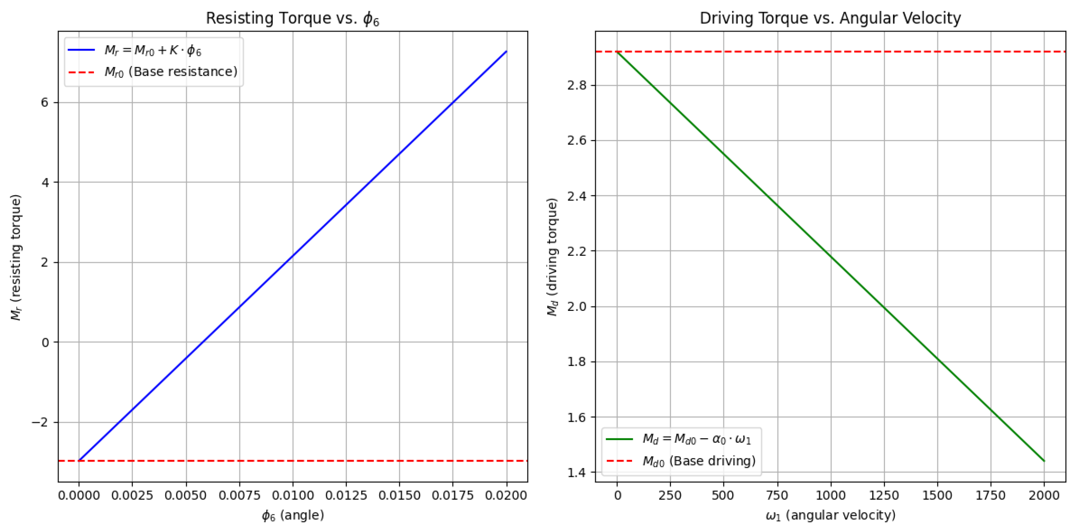
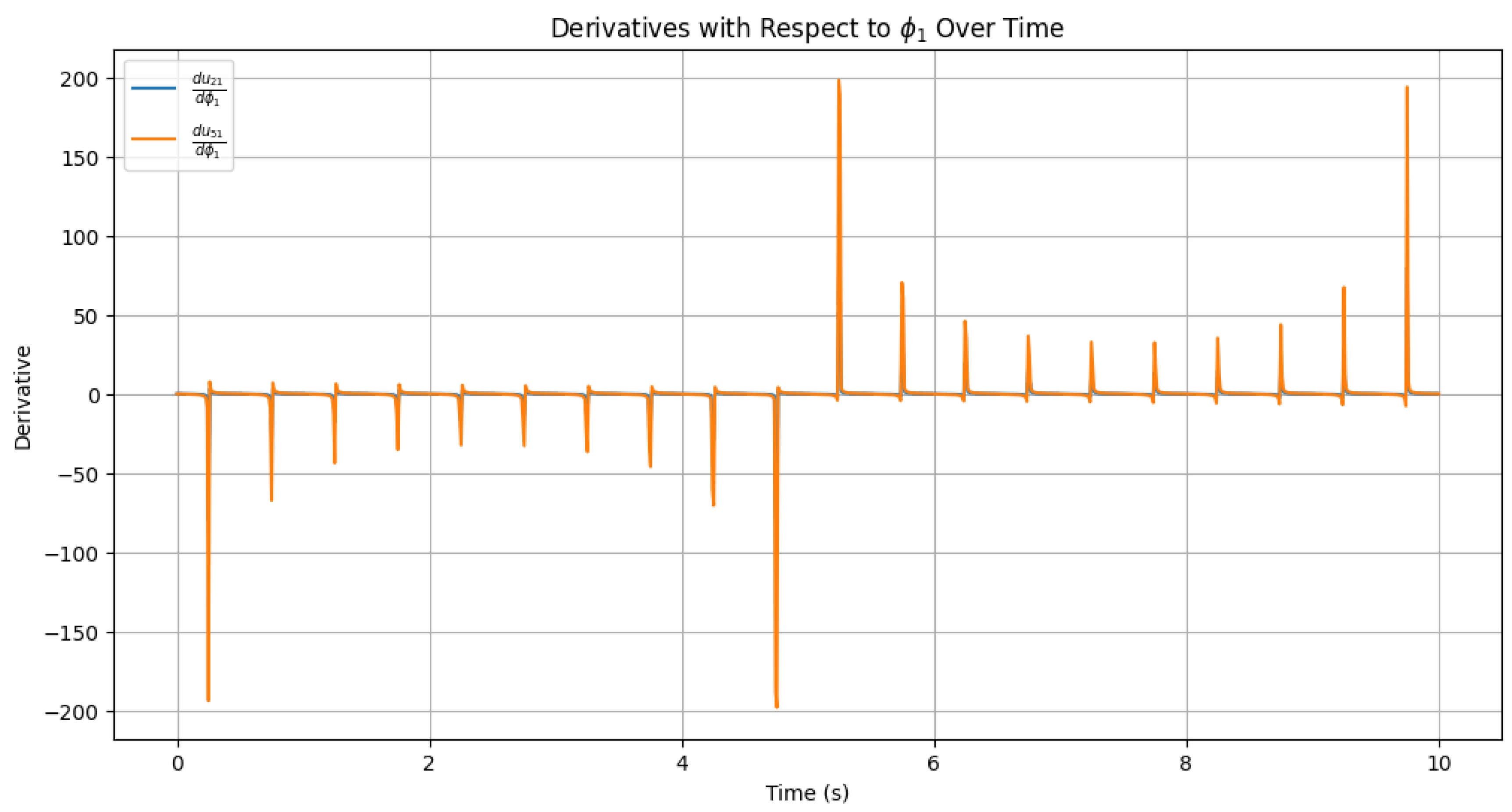
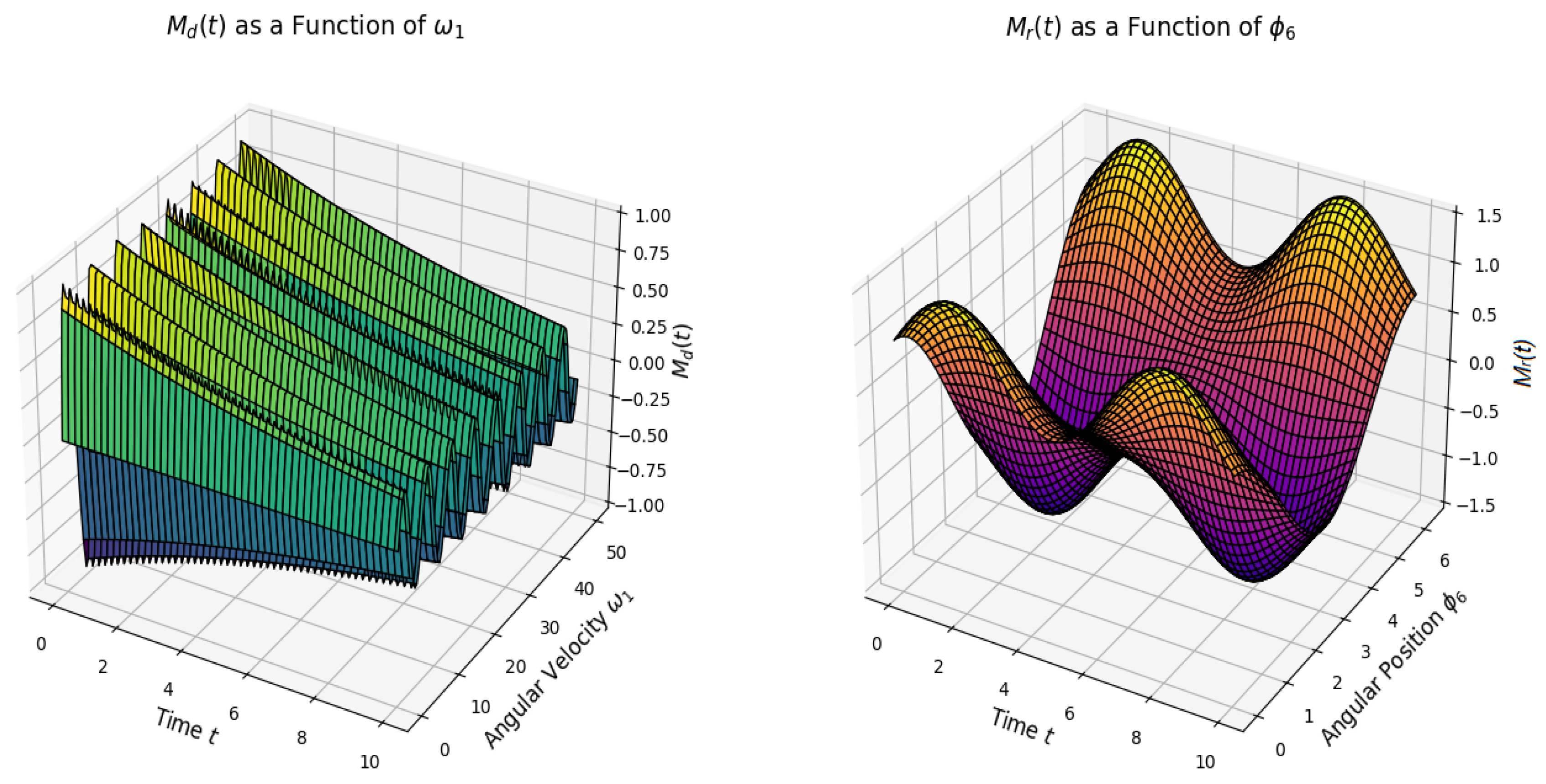
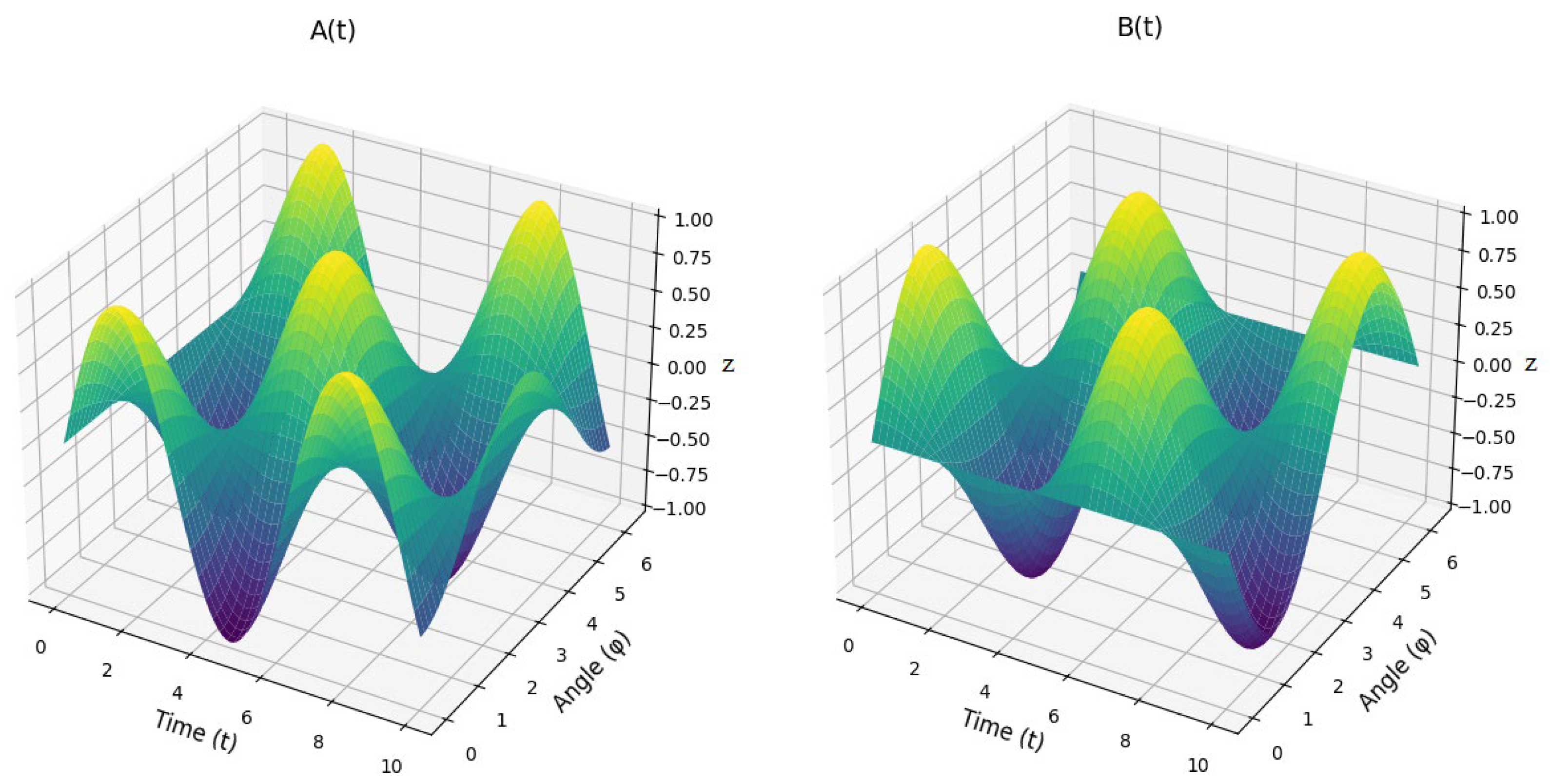
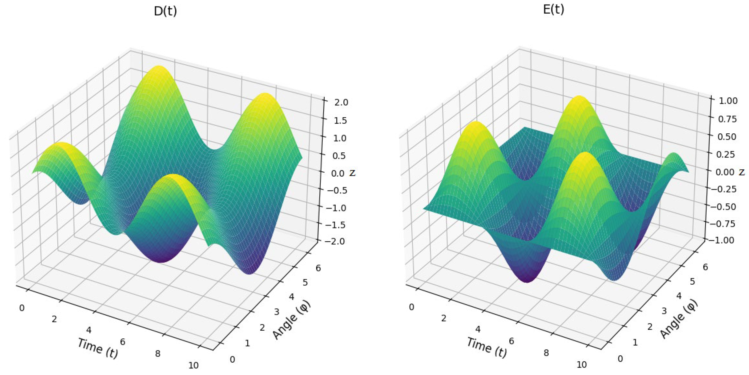
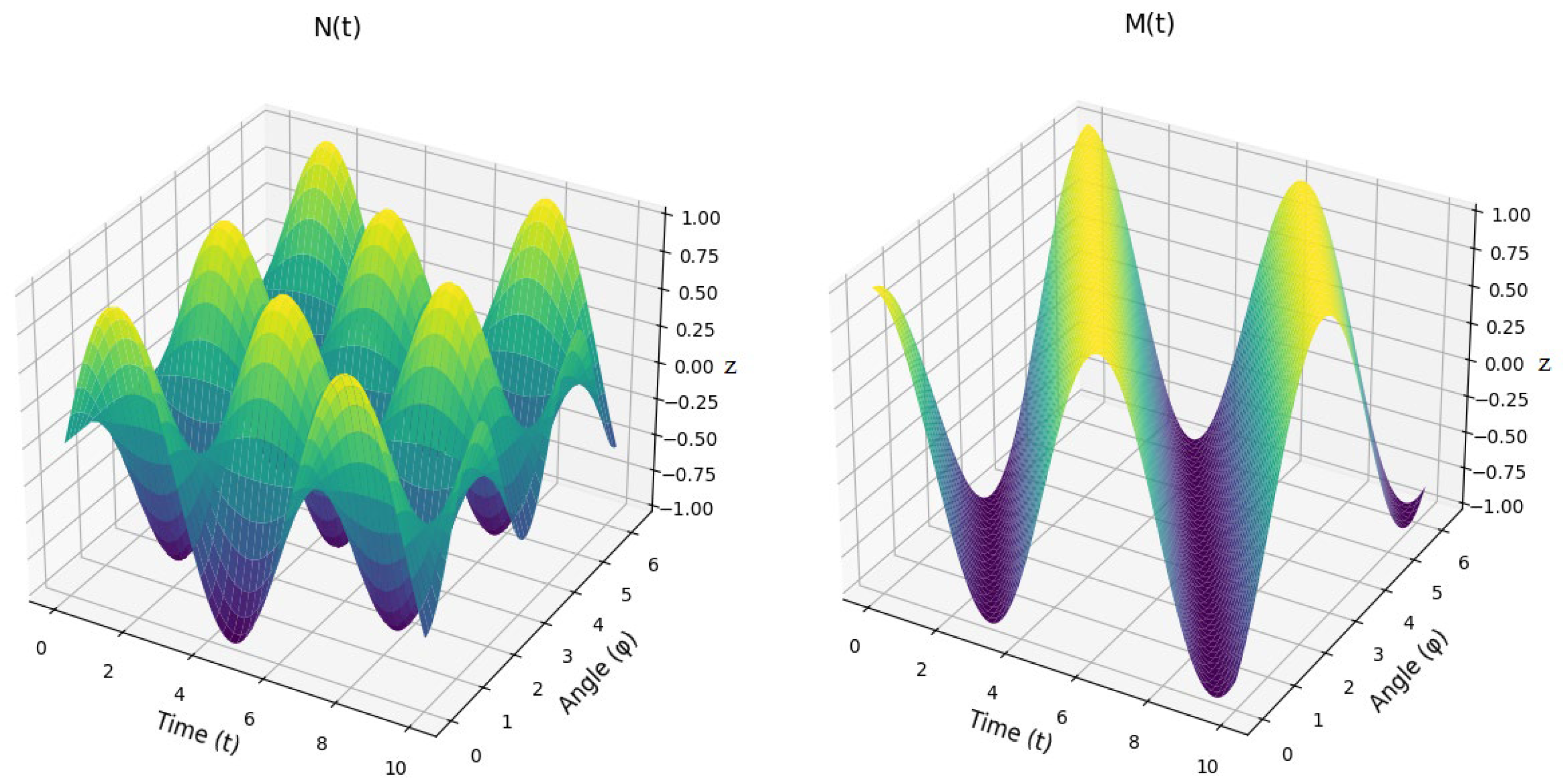
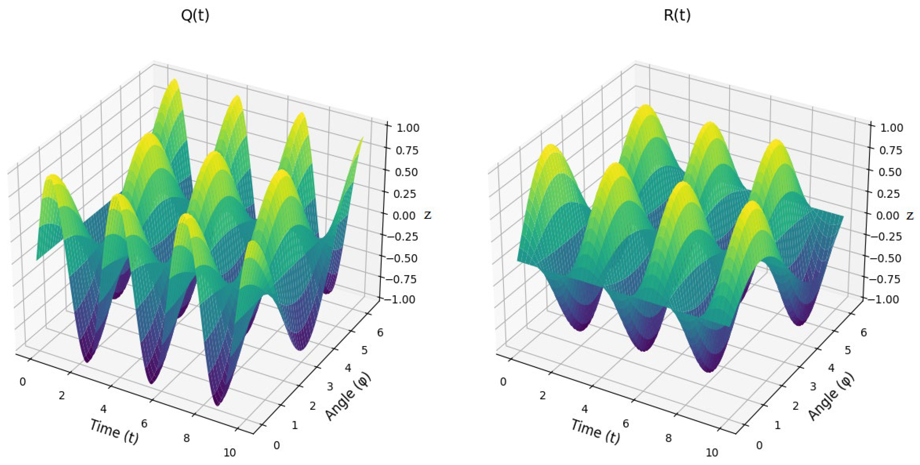
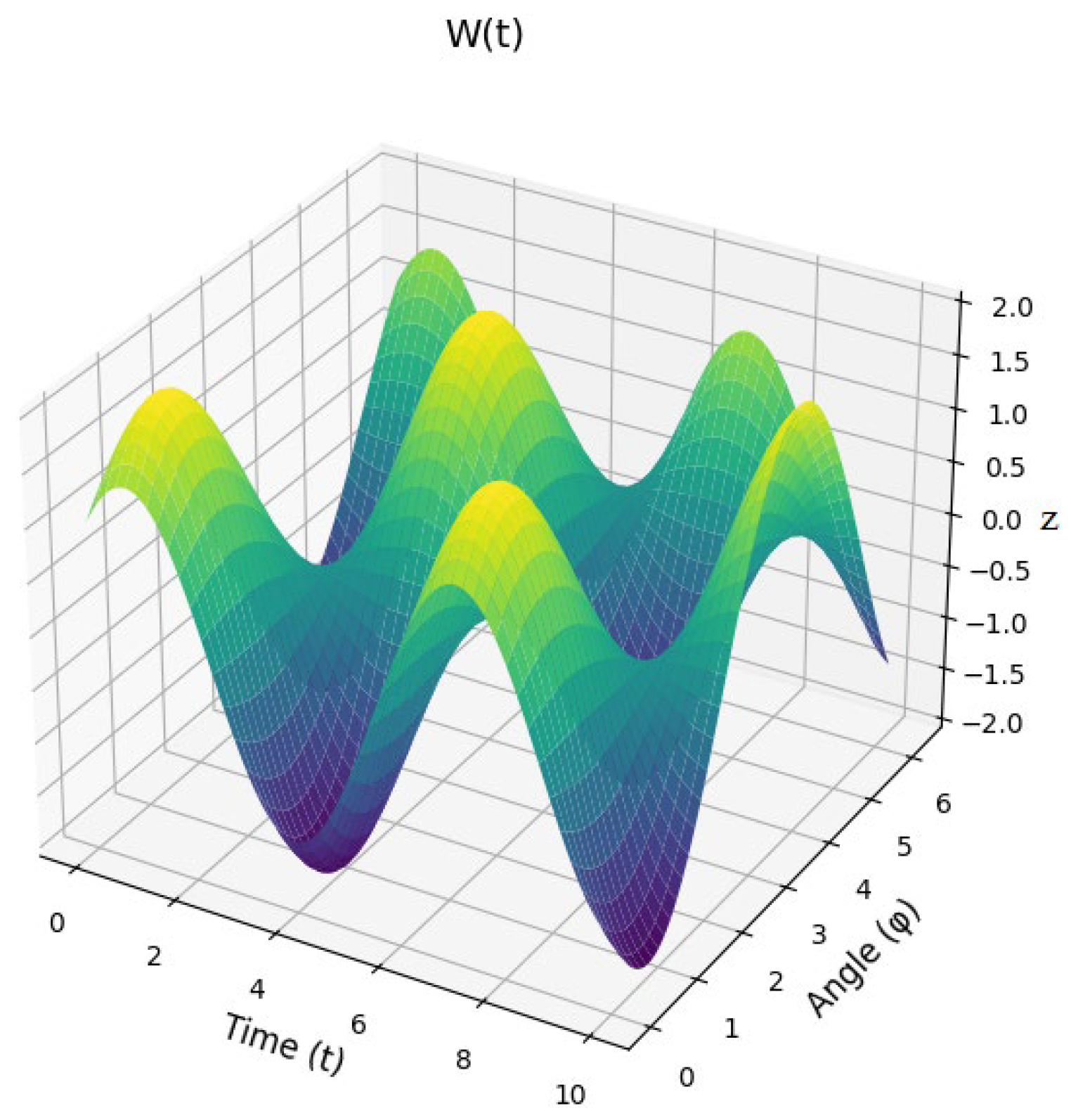
This paper presents a dynamic model for the oscillating conveyor mechanism, governed by a differential equation that describes the system’s motion under the influence of both driving and resisting torques. The resistive torque Mr is modeled as a linear function of angular displacement φ6, while the driving torque Md incorporates a damping term proportional to the angular velocity ω1 . The system’s inertial properties are captured through time-dependent terms such as as A(t), B(t), D(t), E(t), F(t), H(t), N(t), M(t), Q(t), R(t), and W(t), which account for the interaction between the mechanical components, including the angular positions and velocities of the system’s joints. A numerical solution is obtained using an approximate calculation method, specifically an explicit finite difference approach, with initial conditions set to ω0 = 0 and φ0 = 0. This method allows for the computation of angular velocities and displacements over discrete time intervals, providing insight into the system’s dynamic behavior. The results demonstrate the importance of damping and nonlinear dynamics in regulating oscillations, offering a framework for understanding the stability and response of oscillating conveyor mechanisms. The model’s sensitivity to initial conditions and the role of numerical stability are discussed, with suggestions for future work to improve accuracy and applicability in real-world systems.

Keywords: 
;  ;  ;  ;  

1. Introduction

Oscillating conveyor mechanisms are widely used in various industries, such as mining, food processing, and manufacturing, for the transportation and handling of bulk materials. These systems are essential for ensuring efficient [1], continuous movement of materials along a predefined path, often over long distances or through complex processes. The key advantage of oscillating conveyors lies in their ability to minimize material degradation while maintaining high throughput, especially in applications that require precise control of material flow [2]. The performance and reliability of oscillating conveyor systems depend heavily on their kinematic and dynamic characteristics, which govern their motion, stability, and energy consumption. Understanding these characteristics is crucial for optimizing system design, enhancing operational efficiency, and ensuring long-term durability [3]. The kinematic behavior involves the study of the conveyor’s movement, including the velocities, accelerations, and angular displacements of its components. Meanwhile, the dynamic characteristics focus on the forces, torques, and power requirements that influence the system’s operation under different loading conditions. In this research, we aim to explore both the kinematic and dynamic behaviors of an oscillating conveyor mechanism by developing mathematical models that describe the motion of the system’s components [4]. The study incorporates a variety of factors such as link lengths, rotational velocities, external forces, resistive moments, and torque interactions. These parameters are critical for understanding the system’s response to different operational scenarios, including changes in load, oscillation frequency [5], and external disturbances. The research begins by formulating the equations of motion for the conveyor mechanism, using the principles of mechanics and dynamics to describe the system’s response to various forces [6]. These equations are then analyzed to determine the system’s behavior under different conditions, providing valuable insights into the efficiency and stability of the conveyor mechanism. By determining the kinematic and dynamic characteristics [7], this research will not only enhance the understanding of oscillating conveyor systems but also contribute to the development of more efficient designs and control strategies. Ultimately, the findings will have practical implications for improving the performance, energy efficiency, and operational lifespan of oscillating conveyors in industrial applications [8]. The study of dynamic mechanical systems often requires a comprehensive analysis of their kinematic and dynamic characteristics to ensure optimal performance and stability. In the context of oscillatory and rotating mechanisms, such as vibration conveyors or multi-link systems [9], precise mathematical modeling is essential. These systems involve complex interactions between multiple components, where factors like angular velocities, forces, and torques significantly impact performance. In this work, we focus on the dynamic behavior of a vibration conveyor mechanism, characterized by its intricate interdependence of parameters like angular displacements, velocities [10], accelerations, and forces acting on various components. To achieve a detailed understanding of the system, we derive and solve a set of nonlinear differential equations that represent the system’s dynamic behavior [11]. Key parameters, including A ( t ) , B(t), D(t), E(t), F(t), H ( t ) , N(t), M(t), Q ( t ) , R t , and W ( t ) , are explored in terms of their temporal evolution and interdependence. The analysis involves numerical simulations and graphical representation of these parameters, offering insights into the system’s behavior under varying operating conditions. Furthermore, the comparative study of driving and resisting torques [12], M d and M r , highlights the influence of these torques on the overall system dynamics. By leveraging advanced computational techniques and visualization tools, we present 3D plots and comparative analyses that underscore the significance of key parameters in ensuring the stability and efficiency of the mechanism [13]. This investigation not only advances the understanding of oscillatory systems but also provides a robust framework for optimizing their design and control strategies. The findings can be applied to various industrial applications, such as material handling, where precise control of dynamic parameters is critical for operational success.

2. Materials and Methods

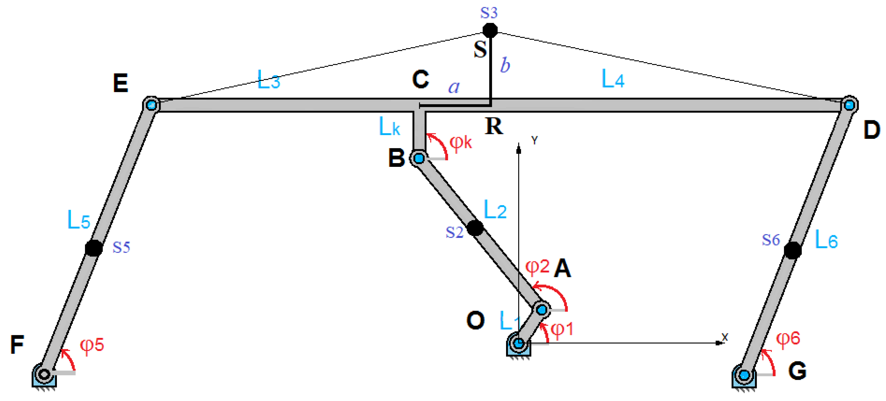
2.1. Geometric and Trigonometric Constraints

The following geometric constraints are applied to ensure proper motion of the mechanism [14]. These equations describe the geometric relationships between the positions and angles of the mechanism components show in Figure 1.
Parameters of the six-link oscillating conveyor mechanism:
L1=OA=60 mm, L2=AB=430 mm, Lk=BC=82 mm, L3=CE=642 mm, L4=CD=1058 mm, L5=L6=EF=DG=440 mm, ED=FG=1700 mm, m1=30 kg, m2=65 kg, m3=1160 kg, m5=m6=59 kg.
For closed contour OABCEFO:
L 1 + L 2 + L k + L 3 = L 7 + L 5
And for closed contour OABCEGO:
L 1 + L 2 + L k = L 8 + L 6 + L 4
These constraints maintain the equilibrium of the system during operation. In addition, trigonometric relationships are used to describe the motion angles φ 1 = φ 1 t , which vary as functions of time. The determination of the kinematic and dynamic parameters for the oscillating conveyor mechanism involves solving a system of nonlinear equations that describe the motion of the mechanism’s components based on given constraints, link lengths, masses, and angular velocities [15].
The vector equation (1) and equation (2) are projected on the Cartesian reference system. It is obtained:
L 1 c o s φ 1 + L 2 c o s φ 2 + L 3 c o s φ 3 = L 7 c o s φ 7 + L 5 c o s φ 5
L 1 s i n φ 1 + L 2 s i n φ 2 + L k + L 3 s i n φ 3 = L 7 s i n φ 7 + L 5 s i n φ 5
L 1 c o s φ 1 + L 2 c o s φ 2 = L 8 c o s φ 8 + L 6 c o s φ 6 + L 4 c o s φ 4
L 1 s i n φ 1 + L 2 s i n φ 2 + L k = L 8 s i n φ 8 + L 6 s i n φ 6 + L 4 s i n φ 4
Additional constraints (assuming φ 3 = φ 4 = 180 ° , φ k = 90 ° , L 5 = L 6 , and φ 5 = φ 6 ):
L 2 c o s φ 2 L 5 c o s φ 5 = L 7 c o s φ 7 L 1 c o s φ 1 + L 3
L 2 s i n φ 2 L 5 s i n φ 5 = L 7 s i n φ 7 L 1 s i n φ 1 L k
Since L 5 = L 6 and φ 5 = φ 6 , you can substitute those relationships to reduce the complexity:
L 2 c o s φ 2 L 5 c o s φ 5 = L 8 c o s φ 8 L 1 c o s φ 1 L 4
L 2 s i n φ 2 L 5 s i n φ 5 = L 8 s i n φ 8 L 1 s i n φ 1 L k
Combine equation (7) and equation (9):
L 7 c o s φ 7 L 1 c o s φ 1 + L 3 = L 8 c o s φ 8 L 1 c o s φ 1 L 4
Combine equation (8) and equation (10):
L 7 s i n φ 7 L 1 s i n φ 1 L k = L 8 s i n φ 8 L 1 s i n φ 1 L k
Simplified System:
L 7 c o s φ 7 + L 3 = L 8 c o s φ 8 L 4
L 7 s i n φ 7 = L 8 s i n φ 8
Using trigonometric identities:
L 7 2 = L 7 c o s φ 7 2 + L 7 s i n φ 7 2
L 8 2 = L 8 c o s φ 8 2 + L 8 s i n φ 8 2
Express φ 8 in terms of φ 7 . From s i n φ 7 = L 8 s i n φ 8 L 7 and c o s φ 7 = L 8 c o s φ 8 L 7 , for φ 8 we solve using:
t a n φ 7 = s i n φ 7 c o s φ 7   and   t a n φ 8 = s i n φ 8 c o s φ 8
The equations describe the geometric and kinematic constraints of the oscillating conveyor mechanism [16], now grouped into simplified forms. Let us organize them and analyze for clarity and solvability.
t g α = O M F M = 40 1325 = 0.03 , α = 1 ° 40 , φ 7 = 180 ° + 1 ° 40 = 181 ° 40 , t g β = M O M G = 40 375 = 0.1066 , β = 6 ° , φ 8 = 360 ° 6 ° = 354 ° , L 3 = 642 mm, L 4 = 1058 mm, L 7 1325.6 mm, L 8 = 337.1 mm.
A and B are determined Eq. (11) and Eq. (12) directly by φ 7 :
A = L 7 c o s φ 7 L 1 c o s φ 1 + L 3
B = L 8 s i n φ 8 L 1 s i n φ 1 L k
These equation link φ 2 and φ 5 using A and B Eq. (9) and Eq. (10):
L 2 c o s φ 2 L 5 c o s φ 5 = A
L 2 s i n φ 2 L 5 s i n φ 5 = B
From the provided constraints:
s i n φ 2 = B + L 5 s i n φ 5 L 2
Using s i n 2 φ 2 + c o s 2 φ 2 =1, substitute s i n φ 2 :
1 c o s 2 φ 2 = B + L 5 s i n φ 5 L 2 2
Rearranging for c o s 2 φ 2 :
c o s 2 φ 2 = 1 B + L 5 s i n φ 5 2 L 2 2
Now, s i n φ 2 becomes:
c o s φ 2 = L 2 2 B + L 5 s i n φ 5 2 L 2 2
The constraint linking φ 2 and φ 5 is:
L 2 c o s φ 2 L 5 c o s φ 5 = A
Substitute c o s φ 2 into this equation:
L 2 L 2 2 B + L 5 s i n φ 5 2 L 2 2 L 5 c o s φ 5 = A
Rearranging for c o s φ 5 :
c o s φ 5 = L 2 L 2 2 B + L 5 s i n φ 5 2 L 2 2 A L 5
Using s i n 2 φ 5 + c o s 2 φ 5 =1, and c o s 2 φ 5 =1- s i n 2 φ 5 :
Squaring both sides of the expression for c o s φ 5 gives:
L 2 L 2 2 B + L 5 s i n φ 5 2 L 2 2 A L 5 2 = 1 s i n 2 φ 5
Simplifying:
Let C = L 2 2 2 A B 2 2 A + A 2 L 5 2 2 A . Expanding the terms results in:
L 2 2 B + L 5 s i n φ 5 2 = C B A L 5 s i n φ 5
Substitute back to form a quadratic equation (29) in s i n φ 5 :
M s i n 2 φ 5 + N s i n φ 5 + P = 0
where M = L 5 2 1 + B 2 A 2 , N = 2 B L 5 1 C A , P = B 2 + C 2 L 2 2
The quadratic formula gives:
s i n φ 5 = N ± N 2 4 M P 2 M = W ,   W = W φ 1
Once s i n φ 5 is determined, φ 5 can be expressed as:
φ 5 = a r c s i n W + 2 π n , φ 5 = f φ 1
Phase angles relationships:
L 2 s i n φ 2 L 5 s i n φ 5 = B
L 2 s i n φ 2 L 5 W = B
s i n φ 2 = B + L 5 W L 2
φ 2 = a r c s i n B + L 5 W L 2 + 2 π n , φ 2 = f φ 1
where φ 5 =f( φ 1 ). Substituting φ 5 ( φ 1 ) into this equation gives φ 2 as a function of φ 1 .
Derivatives, to compute d φ 2 d φ 1 :
d φ 2 d φ 1 = d φ 2 d t d φ 1 d t = ω 2 ω 1 = u 21
Using the chain rule and differentiating φ 2 ( φ 1 ) explicitly will yield the angular velocity ratio u 21 .
Derivatives, to compute d φ 5 d φ 1 :
d φ 5 d φ 1 = d φ 5 d t d φ 1 d t = ω 5 ω 1 = u 51
For the given ratios:
u 21 = L 1 s i n φ 5 φ 1 L 2 s i n φ 2 φ 5
u 51 = L 1 s i n φ 2 φ 1 L 5 s i n φ 2 φ 5
Each u i j depends on the geometric and trigonometric relationships between the angles φ 1 , φ 2 , φ 5 . These relationships can be used to calculate the respective angular velocities.
Angular velocity ratios:
ω 2 ω 1 = u 21 = L 1 s i n φ 5 φ 1 L 2 s i n φ 2 φ 5
ω 5 ω 1 = u 51 = L 1 s i n φ 2 φ 1 L 5 s i n φ 2 φ 5
Similarly, we substitute the corresponding expressions for u 31 , u 41 , u 61 .
Noting that the center of gravity of the third-generation changes according to the law of ellipticity show in Figure 2, the equations for the elliptical motion can be expressed as:
R C = a 0 + a s i n ω 5 t
R S = b 0 + b c o s ω 5 t
RC - is the horizontal position of the center of gravity, varying sinusoidally over time; RS - is the vertical position of the center of gravity, varying cosinusoidally over time; a 0 and b 0 - is the initial positions (offsets) of the center of gravity in the horizontal and vertical directions, respectively; a and b - is the amplitudes of the elliptical motion in the horizontal and vertical directions, respectively; ω 5 - is the angular frequency of the motion [17], determining how quickly the center of gravity traverses the elliptical path; t - is the time variable.
The trajectory described by RC and RS forms an ellipse with:
-
Semi-major axis a (horizontal extent);
-
Semi-minor axis b (vertical extent);
-
Offset determined by a 0 and b 0 , which place the ellipse at a specific location in the coordinate system.
This formulation is often used to describe oscillatory systems with elliptical trajectories, such as oscillating conveyors or mechanisms with rotational and translational motions.
The equations you provided for X S 2 , Y S 2 , X S 3 , and Y S 3 define the coordinates of two points (s2 and s3) in terms of the oscillatory motion variables (RC and RS) and the angular parameters ( φ 1 , φ 2 ):
X S 2 = L 1 c o s φ 1 L 2 c o s φ 2
Y S 2 = L 1 s i n φ 1 + L 2 s i n φ 2
These equations represent the coordinates of a point s2 that depends on the lengths L 1 and L 2 = L 2 2 = A s 2 , as well as the angles φ 1 and φ 2 . This is a purely kinematic representation, without any influence of oscillatory displacements.
X S 2 ˙ = L 1 s i n φ 1 d φ 1 d t + L 2 s i n φ 2 d φ 2 d t = L 1 s i n φ 1 d φ 1 d t + L 2 s i n φ 2 d φ 2 d t d φ 1 d t = L 1 s i n φ 1 + L 2 s i n φ 2 u 21 ω 1
Y S 2 ˙ = L 1 c o s φ 1 d φ 1 d t + L 2 c o s φ 2 d φ 2 d t = L 1 c o s φ 1 d φ 1 d t + L 2 c o s φ 2 d φ 2 d t d φ 1 d t = L 1 c o s φ 1 + L 2 c o s φ 2 u 21 ω 1
To determine the magnitude of velocity ϑ S 2 , we use the formula for the resultant velocity from its components along the X- and Y-directions:
ϑ S 2 = X S 2 ˙ 2 + Y S 2 ˙ 2 = ω 1 L 1 2 + L 1 L 2 u 21 c o s φ 1 φ 2 + 2 L 2 2 u 21 2
To determine ϑ S 3 , the velocity magnitude of point s3, we follow a similar approach to earlier calculations. The velocity components in the X- and Y-directions are given by. To calculate ϑ S 3 , the magnitude of the velocity at point s3, given the components X S 3 ˙ and Y S 3 ˙ , we follow these steps:
ϑ S 3 = X S 3 ˙ 2 + Y S 3 ˙ 2 = ω 1 2 { L 1 s i n φ 1 + L 2 s i n φ 2 u 21 2 + L 1 c o s φ 1 + L 2 c o s φ 2 u 21 2 2 L 1 s i n φ 1 + L 2 s i n φ 2 u 21 a u 51 c o s ω 5 t 2 L 1 c o s φ 1 + L 2 c o s φ 2 u 21 b u 51 s i n ω 5 t + a u 51 c o s ω 5 t 2 + b u 51 s i n ω 5 t 2 }
d ϑ S 2 d φ 1 = d d φ 1 ( L 1 sin φ 1 + L 2 sin φ 2 u 21 ) 2 + ( L 1 cos φ 1 + L 2 cos φ 2 u 21 ) 2 ω 1 =
= ω 1 L 1 cos φ 1 + L 2 cos φ 2 u 21 2 L 1 sin φ 1 L 2 sin φ 2 u 21 2 + L 2 sin φ 2 d u 21 d φ 1 + L 2 cos φ 2 d u 21 d φ 1 L 1 sin φ 1 + L 2 sin φ 2 u 21 2 + L 1 cos φ 1 + L 2 cos φ 2 u 21 2 =
= ω 1 L 1 cos φ 1 sin φ 1 + L 2 cos φ 2 sin φ 2 u 21 2 + L 2 d u 21 d φ 1 sin φ 2 + cos φ 2 L 1 sin φ 1 + L 2 sin φ 2 u 21 2 + L 1 cos φ 1 + L 2 cos φ 2 u 21 2
d ϑ S 3 d φ 1 = d d φ 1 L 1 sin φ 1 L 2 sin φ 2 u 21 + a u 51 cos ω 5 t 2 + L 1 cos φ 1 + L 2 cos φ 2 u 21 b u 51 sin ω 5 t 2 ω 1 =
= ω 1 L 1 cos φ 1 L 2 cos φ 2 u 21 2 L 2 sin φ 2 d u 21 d φ 1 + a cos ω 5 t d u 51 d φ 1 L 1 sin φ 1 L 2 sin φ 2 u 21 2 + L 2 cos φ 2 d u 21 d φ 1 b sin ω 5 t d u 51 d ϕ 1 L 1 sin φ 1 + L 2 sin φ 2 u 21 a u 51 cos ω 5 t 2 + L 1 cos φ 1 + L 2 cos φ 2 u 21 b u 51 sin ω 5 t 2
= ω 1 L 1 sin φ 1 + cos φ 1 L 2 u 21 2 cos φ 2 + sin φ 2 + L 2 d u 21 d φ 1 cos φ 2 sin φ 2 + d u 51 d φ 1 a cos ω 5 t b sin ω 5 t L 1 sin φ 1 + L 2 sin φ 2 u 21 a u 51 cos ω 5 t 2 + L 1 cos φ 1 + L 2 cos φ 2 u 21 b u 51 sin ω 5 t 2
u 21 = L 1 ( cos φ 1 sin φ 5 cos φ 5 sin φ 1 ) L 2 ( sin φ 2 cos φ 5 cos φ 2 sin φ 5 )
d u 21 d φ 1 = L 1 L 2 u 51 cos φ 5 cos φ 1 sin φ 5 sin φ 1 cos φ 1 cos φ 5 + sin φ 1 sin φ 5 u 51 sin φ 2 cos φ 5 cos φ 2 sin φ 5 cos φ 1 sin φ 5 sin φ 1 cos φ 5 cos φ 2 cos φ 5 u 21 sin φ 2 sin φ 5 u 51 + sin φ 2 sin φ 5 u 21 cos φ 2 cos ϕ 5 u 41 sin φ 2 cos φ 5 sin φ 5 cos φ 2 2
= L 1 L 2 u 51 cos φ 5 φ 1 cos φ 5 φ 1 sin φ 5 φ 2 sin φ 5 φ 1 u 21 cos φ 5 φ 1 u 21 cos φ 5 φ 2 sin 2 φ 5 φ 2 =
= L 1 L 2 cos φ 5 φ 1 u 51 cos φ 5 φ 1 sin φ 5 φ 2 u 21 cos φ 5 φ 2 u 51 cos φ 5 φ 2 sin φ 5 φ 1 sin 2 φ 5 φ 2
u 51 = L 1 ( cos φ 1 sin φ 2 sin φ 1 cos φ 2 ) L 5 ( cos φ 5 sin φ 2 sin φ 5 cos φ 2 )
d u 51 d φ 1 = L 1 L 5 sin φ 1 sin φ 2 + cos φ 1 cos φ 2 u 21 cos φ 1 cos φ 2 + sin φ 1 sin φ 2 u 21 sin φ 5 φ 2 sin φ 2 φ 1 sin φ 5 sin φ 2 u 51 + cos φ 5 cos φ 2 u 21 + sin φ 5 sin φ 2 u 21 cos φ 5 cos φ 2 u 51 sin 2 φ 5 φ 2 =
= cos φ 2 φ 1 u 21 cos φ 2 φ 1 sin φ 5 φ 2 sin φ 2 φ 1 cos φ 5 φ 2 u 21 cos φ 5 φ 2 u 51 sin 2 φ 5 φ 2

2.2. Differential Equations of Motion of the Joints of an Oscillating Conveyor Mechanism

Equation for joint 1 motion:
I d ( φ 1 ) d ω 1 d t = ω 1 2 2 d Ι d ( φ 1 ) d φ 1 = M d М r
where M d .- is the driving torque; М r   - is the resisting torque.
The driving torque on the joint is related to the torques from different components (such as M E r , M D r , М F r , and M G r ):
where M E r , M D r , М F r , and M G r is the are the resisting torques from different parts of the system; ω 5 and ω 6 is the are the angular velocities of the respective components [18].
M d ω 1 = M E r ω 5 + M D r ω 6 + М F r ω 5 + M G r ω 6
By substituting and factoring the terms in the equation for M d , we get:
M d = M E r ω 5 ω 1 + М D r ω 6 ω 1 + М F r ω 5 ω 1 + М G r ω 6 ω 1
Which can be simplified further to:
M d = M E r u 51 + М D r u 61 + M F r u 51 + M G r u 61 = 4 u 51 M r
where u 51 and u 61 are terms relating to the motion of the system, possibly dependent on the geometry or kinematic relationships between different components.
The motion of the oscillating conveyor mechanism is driven by the external torques M d , which depend on the angular velocities of different parts of the system. These equations couple the rotational dynamics of joint 1 with the other components in the system.
M r =   M r 0 + К φ 6
M r 0 - is the base moment of the applied resistance force (perhaps considering some other factors), M r 0 = 2.98 and this value represents the inherent resisting torque in the system at φ 6 = 0 ; K - is the stiffness coefficient related to the change in M r with respect to φ 6 . A higher K indicates a steeper increase in resistance torque as φ 6 increases; φ 6 - is the parameter (angle) representing the system’s configuration or deformation, directly affecting M r .
Expression for K:
K = t g α = 14.86 5.94 2 ° 1 ° = 8.92 0.017453 = 511.84
This constant K is calculated using the tangent of angle α, and it equals 511.84, which plays a key role in determining how the driving torque depends on φ 6 .
The formula for M r is given by:
φ 6 = φ 6 ( φ 1 ) , M r = M r ( φ 1 ) ; M r = 2.98 + 511.87 φ 6
where M r 0 - is the expressed as a linear function of φ 6 ; the constant −2.98 represents an offset, 511.84 is the sensitivity factor, which amplifies the effect of φ 6 on the driving torque. At φ 6 = 0 , the resisting torque M r equals −2.98, representing a baseline resistance. As ϕ6 increases, M r grows linearly due to the stiffness coefficient K. This behavior reflects how the resistance increases proportionally to the angular displacement φ 6 .
Using the expression for M d 0 , the driving torque M d becomes. The driving torque M d is expressed as:
M d = М d ο α 0 ω 1
where α 0 – is the coefficient representing the rate at which driving torque decreases with increasing angular velocity. This accounts for damping effects, ω 1 - is the angular velocity of joint 1, М d ο - is the base moment of the applied driving force ( M d ο = 2.92 ) . This is the driving torque when the angular velocity ω 1 = 0 . At ω 1 = 0 increases, M d decreases linearly due to the damping effect represented by α 0 . This reflects energy loss or reduced efficiency as the system accelerates. The final equation also includes a damping or resisting term proportional to the angular velocity ω 1 , with a constant α 0 . This structure allows you to compute the driving torque in terms of the angular position and velocity of the system components, which are key to understanding the dynamics of the oscillating conveyor mechanism [19]. The first subplot shows the relationship between M r and φ 6 . The second subplot shows the relationship between M d and ω 1 show in Figure 3. Resisting Torque ( M r ) Calculated for a range of φ 6 values (0 to 0.02 rad) based on the formula M r = 2.98 + 511.87 φ 6 . Driving Torque ( M d ) Calculated for a range of ω 1 values (0 to 2000 rad/s) based on the formula M d = 2 . 92 0 . 00074 ω 1 .
Let’s break down the equations step by step:
α 0 = t g α = 2,8 1,8 1500 150 = 1 1350 = 0,00074
Given values:
Y =2.92, Y 1 =2.8, Y 2 =1.8, X 1 =150, X 2 =1500, M r =2.92
Linear relationship equation:
Y Y 1 Y 2 Y 1 = Χ Χ 1 Χ 2 Χ 1
This is a form of linear interpolation or a proportionality equation, where X and Y are related within the intervals [X1, X2] and [Y1, Y2]. Substituting the values:
Y 2,8 1,8 2,8 = Χ 150 1500 150
Simplifying the left-hand side:
0 . 12 1 = Χ 150 1350
0.12 = Χ 150 1350
So, X=−12.
Now, based on we last expression:
M d = 2 . 92 0 . 00074 ω 1
This shows that the driving torque M d depends on the angular velocity ω 1 , with a small damping effect due to the factor α 0 .
To ensure the system operates stably:
The driving torque M d must overcome the resisting torque M r . This establishes the condition for motion.
The equations show that M r grows with φ 6 , while M d decreases with ω 1 . A balance is achieved when the two torques are equal.
This analysis provides a foundation for understanding and optimizing the torques in the oscillating conveyor mechanism. The interaction between M r and M d governs the system’s behavior. If M d < M r , the system will decelerate or stop. Conversely, if M d > M r , the system will accelerate.
Moment of inertia Ι d ( φ 1 ) :
Ι d ( φ 1 ) = Ι S 1 + m 2 ϑ S 2 φ 1 + Ι S 2 u 21 2 + m 3 ϑ S 3 φ 1 2 + ( Ι 5 F + Ι 6 G ) L 5 2
where Ι S 1 – is the moment of inertia of the first component; Ι S 2 – is the moment of inertia of the second component; Ι 5 F - is the combined moment of inertia of the fifth component; Ι 6 G is the combined moment of inertia of the sixth component; m 2 ϑ S 2 and m 3 ϑ S 3 – is the terms accounting for the contributions of specific masses m 1 and m 3 at velocities ϑ S 2 and ϑ S 3 respectively; u 21 and u 51 - is the ratios representing relationships between components in the system.
Components:
Ι S 1 = m 1 L 1 2 2
Ι S 2 = m 2 L 2 2 2
Ι 5 F = Ι S 5 + m 5 L 5 = m 5 L 5 2 2 + m 5 L 5 2 4
Ι 6 G = Ι S 6 + m 6 L 6 = m 6 L 6 2 2 + m 6 L 6 2 4
To differentiate the given moment of inertia Ι k ( φ 1 ) with respect to φ 1 , differentiation with respect to φ 1 :
d Ι k ( φ 1 ) d φ 1 = 2 m 2 ( L 1 sin φ 1 + L 2 sin φ 2 u 21 ) 2 + ( L 1 cos φ 1 + L 2 cos φ 2 u 21 ) 2 ω 1
ω 1 L 1 cos φ 1 sin φ 1 + L 2 u 21 2 cos φ 2 sin φ 2 + L 2 d u 21 d φ 1 sin φ 2 + cos φ 2 L 1 sin φ 1 + L 2 sin φ 2 u 21 2 + L 1 cos φ 1 + L 2 cos φ 2 u 21 2 + 2 I S 2 L 1 L 2 sin φ 5 φ 1 sin φ 2 φ 1
L 1 L 2 u 51 cos φ 5 φ 1 cos φ 5 φ 1 sin φ 5 φ 2 u 21 cos φ 5 φ 2 u 51 cos φ 5 φ 2 sin φ 5 φ 1 sin 2 φ 5 φ 2 +
+ 2 m 3 ω 1 2 [ L 1 cos φ 1 + sin φ 1 L 2 u 21 2 cos φ 2 sin φ 2 + L 2 d u 21 d φ 1 cos φ 2 sin φ 2 + d u 51 d φ 1 a cos ω 5 t b sin ω 5 t ]
+ 2 I 5 F + I 6 G L 1 L 5 { cos φ 1 φ 2 u 21 cos φ 1 φ 2 sin φ 2 φ 5 cos φ 1 φ 2 u 21 cos φ 1 φ 2 sin φ 2 φ 1 sin 2 φ 2 φ 5 } L 1 L 5 sin ( φ 2 φ 1 ) sin ( φ 2 φ 5 )
= 2 m 2 ω 1 2 L 1 cos φ 1 sin φ 1 + L 2 u 21 cos φ 2 sin φ 2 + L 2 d u 21 d φ 1 sin φ 2 cos φ 2 +
+ 2 Ι S 2 L 1 2 L 2 2 sin ( φ 5 φ 1 ) sin ( φ 2 φ 5 ) { u 51 cos φ 1 φ 5 cos φ 5 φ 1 sin φ 2 φ 5 u 21 cos φ 5 φ 2 u 51 cos φ 5 φ 2 sin φ 5 φ 1 sin 2 φ 5 φ 2
2 m 3 ω 1 2 [ L 1 cos φ 1 + sin φ 1 + L 2 u 21 2 cos φ 2 sin φ 2 L 2 d u 21 d φ 1 sin φ 2 cos φ 2 d u 51 d φ 1 a cos ω 5 t b sin ω 5 t ]
+ 2 I 4 F + I 5 G L 1 2 L 4 2 sin ( φ 2 φ 1 ) sin ( φ 2 φ 5 ) cos φ 1 φ 2 u 21 cos φ 1 φ 2 sin φ 2 φ 5 cos φ 1 φ 2 u 21 cos φ 1 φ 2 sin φ 2 φ 1 sin 2 φ 2 φ 5
The rate of change of Ι k ( φ 1 ) depends on the relationships d ϑ S 2 d φ 1 , d ϑ S 3 d φ 1 , d u 21 d φ 1 and d u 51 d φ 1 . The applied equation of motion is as follows:
Ι S 1 + m 2 ω 1 2 L 1 sin φ 1 + L 2 sin φ 2 u 21 2 + L 1 cos φ 1 + L 2 cos φ 2 u 21 2 + Ι S 2 L 1 2 L 2 2 sin 2 ( φ 4 φ 1 ) sin 2 ( φ 2 φ 4 ) +
+ m 3 ω 1 2 L 1 sin φ 1 L 2 sin φ 2 u 21 + a u 51 cos ω 5 t 2 + l 1 cos φ 1 + l 2 cos φ 2 u 21 b u 51 sin ω 5 t 2 +
+ ( Ι 5 F + Ι 6 G ) L 1 2 L 5 2 sin 2 ( φ 2 φ 1 ) sin 2 ( φ 2 φ 5 ) d ω 1 d t + ω 1 2 2 2 m 2 ω 1 2 ( L 1 sin φ 1 + L 2 sin φ 2 u 21 ) ( L 1 cos φ 1 u 21 2 + L 2 sin φ 2 d u 21 d φ 1 ) +
+ ( L 1 cos φ 1 + L 2 cos φ 2 u 21 ) ( L 1 sin φ 1 L 2 sin φ 2 u 21 2 + L 2 cos φ 2 d u 21 d φ 1 ) +
+ 2 Ι S 2 L 1 2 L 2 2 ( cos ( φ 1 + φ 5 ) cos ( φ 1 + φ 5 ) ) sin ( φ 1 φ 5 ) sin 2 ( φ 2 φ 5 ) + 2 m 3 ω 1 2 L 1 sin φ 1 L 2 sin φ 2 u 21 + a u 51 cos ω 5 t ) L 1 cos φ 1 L 2 cos φ 2 u 21 2 L 1 sin φ 2 d u 21 d φ 1 + a cos ω 5 t d u 51 d φ 1 +
+ ( L 1 cos φ 1 + L 2 cos φ 2 u 21 b u 51 sin ω 5 t ) L 1 sin φ 1 + L sin φ 2 u 21 2 + L 2 cos φ 2 d u 21 d φ 1 b sin ω 5 t d u 51 d φ 1 +
+ ( Ι 5 F + Ι 6 G ) 2 L 1 2 L 2 2 cos ( φ 1 + φ 2 ) cos ( φ 1 φ 2 ) sin ( φ 2 φ 1 ) sin 2 ( φ 2 φ 5 ) =
= M d ο α ω 1 4 u 51 ( M r 0 + K φ 6 )
Given the initial conditions t=0, ω 1 = 0 , and φ 1 = 0 , we aim to solve the equations that describe the system dynamics. Here’s a step-by-step guide to proceed with the solution.

2.3. Solving the Differential Equation of an Oscillating Conveyor Mechanism Using the Approximate Calculation Method

The problem involves solving a complex nonlinear differential equation for the dynamics of a mechanical system [20], where angular velocity ( ω 1 ) and angle ( φ 1 ) evolve over time under the influence of inertia, resistance, and driving forces. The equation is expressed as:
R ( t ) d ω 1 d t + Q ( t ) ω 2 ( t ) = W ( t )
with R t ,   Q ( t ) , and W ( t ) defined as functions of system parameters, geometry, and time. The solution incorporates initial conditions (t=0, ω 1 = 0 , and φ 1 = 0 ) and relies on numerical approximation methods [21].
where R ( t ) – is the represents the combined system inertia and dynamic effects; Q ( t ) - is the accounts for quadratic velocity-dependent effects; W ( t ) – is the Represents the driving force, including torques and damping effects. The solution requires numerically evaluating R ( t ) , Q ( t ) , and W ( t ) based on the provided relationships.
R ( t ) = Ι S 1 + ( m 2 A ( t ) + m 3 H ( t ) ω 1 2 + B ( t ) + D ( t )
R ( t ) is the encapsulates the combined effects of system mass and dynamic configurations. Terms such as A ( t ) and H ( t ) involve trigonometric and geometric dependencies, linking lengths L i angles φ i and oscillatory terms. Q ( t ) represents quadratic velocity-dependent effects and includes contributions from terms E ( t ) , F ( t ) , N ( t ) and M ( t ) , which are influenced by angular relationships and material properties. W ( t ) integrates external forces, damping, and oscillatory effects. It is directly influenced by torque M r and damping coefficients α .
This algorithm (Table 1) uses iterative numerical integration to solve the motion of the oscillating conveyor mechanism [22] over a series of discrete time steps. By calculating the system’s dynamics step by step, it provides the angular velocity and displacement for each time step, ultimately leading to the desired system behavior over time. The key steps include updating the velocity and displacement using time-dependent parameters, followed by a check to continue the iteration or end the process based on the number of steps.
The expression for A ( t ) is given as:
A ( t ) = L 1 2 + 2 L 1 L 2 ( sin φ 1 sin φ 2 + cos φ 1 cos φ 2 ) u 21 + L 2 2 u 21 2
A ( t ) - is the contributes to the inertia and energy terms of the system, making it crucial in describing dynamic behaviors.
H t = L 1 2 L 2 2 u 21 2 + a 2 cos 2 ω 5 t + b 2 sin 2 ω 5 t u 51 2 + 2 L 1 L 2 u 21 sin φ 1 sin φ 2 + cos φ 1 cos φ 2
2 L 1 u 51 ( a sin φ 1 cos ω 5 t + b cos φ 2 sin ω 5 t ) 2 L 2 u 21 ( a cos ω 5 t sin φ 2 + b sin ω 5 t cos φ 2 )
H ( t ) – is the governs dynamic inertia contributions from the links, angles, and elliptical motion components.
u 51 = u 61 = L 1 sin ( φ 2 φ 1 ) L 5 sin ( φ 2 φ 5 )
u 21 = L 1 sin ( φ 5 φ 1 ) L 2 sin ( φ 2 φ 5 )
B ( t ) = Ι S 2 L 1 2 sin 2 ( φ 5 φ 1 ) L 2 2 sin 2 ( φ 2 φ 5 )
B(t) - is the represents the rotational effect of link 2 influenced by angular positions φ 5 , φ 1 , φ 2 .
D ( t ) = ( Ι 5 F + Ι 6 G ) L 1 2 sin 2 ( φ 2 φ 1 ) L 5 2 sin 2 ( φ 2 φ 5 )
D(t) - is the accounts for the combined inertial effects of links 5 and 6 modulated by relative angles φ 1 , φ 2 , φ 5 .
Q ( t ) = ( m 2 E ( t ) + m 3 F ( t ) ) 2 ω 1 2 + 2 Ι S 2 L 1 2 L 2 2 N ( t ) + M ( t )
Q ( t ) - are the accounts for quadratic velocity-dependent effects. Q ( t ) represents quadratic velocity-dependent effects and includes contributions from terms E ( t ) , F ( t ) ,   N ( t ) and M ( t ) , which are influenced by angular relationships and material properties.
E ( t ) = ( L 1 sin φ 1 + L 2 1 sin φ 2 u 21 ) L 1 cos φ 1 + L 2 1 cos φ 2 u 21 2 + L 2 1 sin φ 2 d u 21 d φ 1 +
+ L 1 cos φ 1 + L 2 1 cos φ 2 u 21 L 1 sin φ 1 L 2 1 sin φ 2 u 21 2 + L 2 1 cos φ 2 d u 21 d φ 1
E(t) - is the energy term tied to angular positions and coupling ratios.
F t = L 1 sin φ 1 L 2 sin φ 2 u 21 + a u 51 cos ω 5 t ( L 1 cos φ 1 L 2 cos φ 2 u 21 2 L 1 sin φ 1 d u 21 d φ 1 + a cos ω 5 t d u 51 d φ 1 +
+ ( L 1 cos φ 1 + L 2 cos φ 2 u 21 b u 51 sin ω 5 t ) ( L 1 sin φ 1 L 2 sin φ 2 u 21 2 + L 2 cos φ 2 d u 21 d φ 1 b sin ω 5 t d u 51 d φ 1 )
F(t) - is the damping and inertial effects with oscillatory external inputs.
N ( t ) = ( cos ( φ 1 + φ 5 ) cos ( φ 1 φ 1 ) ) sin ( φ 1 φ 5 ) sin 2 ( φ 2 φ 5 )
N(t) - is the coupling strength based on angular misalignments.
M ( t ) = ( Ι 5 F + Ι 6 G ) 2 L 1 2 L 2 2 ( cos ( φ 1 + φ 2 ) cos ( φ 1 φ 2 ) ) sin ( φ 2 φ 1 ) sin 2 ( φ 2 φ 5 )
M(t) – is the torque contribution influenced by inertia and geometry.
W ( t ) = M d ο α ω 1 4 u 51 ( M r 0 + K φ 6 )
Given your detailed numerical approximation method for solving the differential equation:
ω 0 = 0 , φ 0 = 60 ° , h=0.01, k=0,1,2…N-1, t k = k h , ω k = ω t k for k=0,1…N.
Approximation of the differential equation:
R k ω k + 1 ω k h + Q k ω k 2 = W k
where h - is the time step size; ω – is the angular velocity at the time step t k ; W k , R k , and Q k are the corresponding values at t k .
Simplifies to:
ω k + 1 = ω k + h W k R k Q k R k ω k 2
Angular position update for φ k . The angular position φ t is related to the angular velocity ω t . As per the equation:
φ k + 1 = φ k + h ω k
This is a simple update based on the angular velocity at each step.
For each time step, we iteratively calculate the angular velocity ω k and the angular position φ k . The total simulation time is divided into N steps, and the time step h determines the accuracy of the approximation. Initial conditions are specified at t=0: ω 0 = 0 and φ 0 = 0 . The equation of motion is discretized using the Euler method, leading to the iterative formulas for ω k + 1 and φ k + 1 . Stability of the solution depends on the choice of step size h, with smaller values yielding more accurate results at the cost of increased computational time. The accuracy of the method is first-order, meaning the error decreases quadratically with the step size h. The computational efficiency is an important consideration, especially if the system is large or requires many time steps [2]. This analysis demonstrates a comprehensive approach to solving and interpreting the dynamics of a nonlinear mechanical system using numerical methods [23]. The results highlight the interplay between inertia, resistance, and driving forces, providing valuable insights into the system’s behavior and stability under different conditions. The comparative analysis of the driving and resisting moments provides a detailed understanding of the system’s dynamics. Through this comparison, one can gain insights into the forces governing system motion, identify potential stability concerns, and optimize the system for performance and efficiency. Numerical simulations offer a powerful tool for visualizing these interactions, and through careful analysis of the results, engineers can make informed decisions about system design, energy efficiency, and control strategies.

3. Methodology

The analysis of the vibration conveyor mechanism was conducted in three main stages: kinematic analysis, dynamic analysis [24], and numerical approximation [17]. The methodologies applied at each stage are as follows:
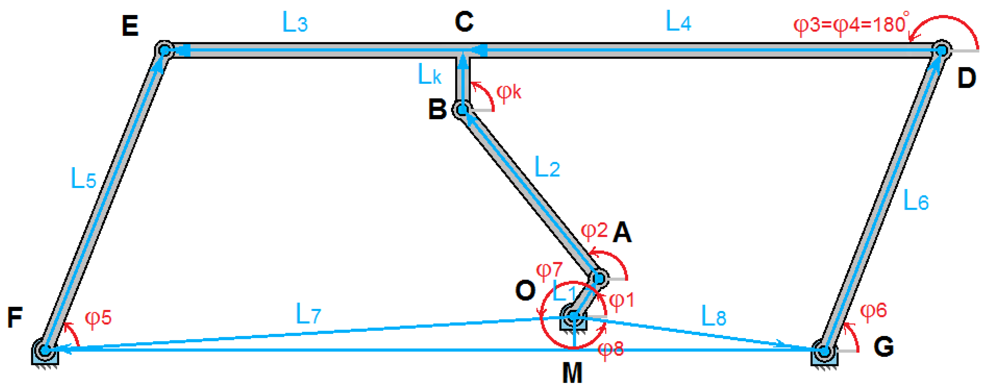
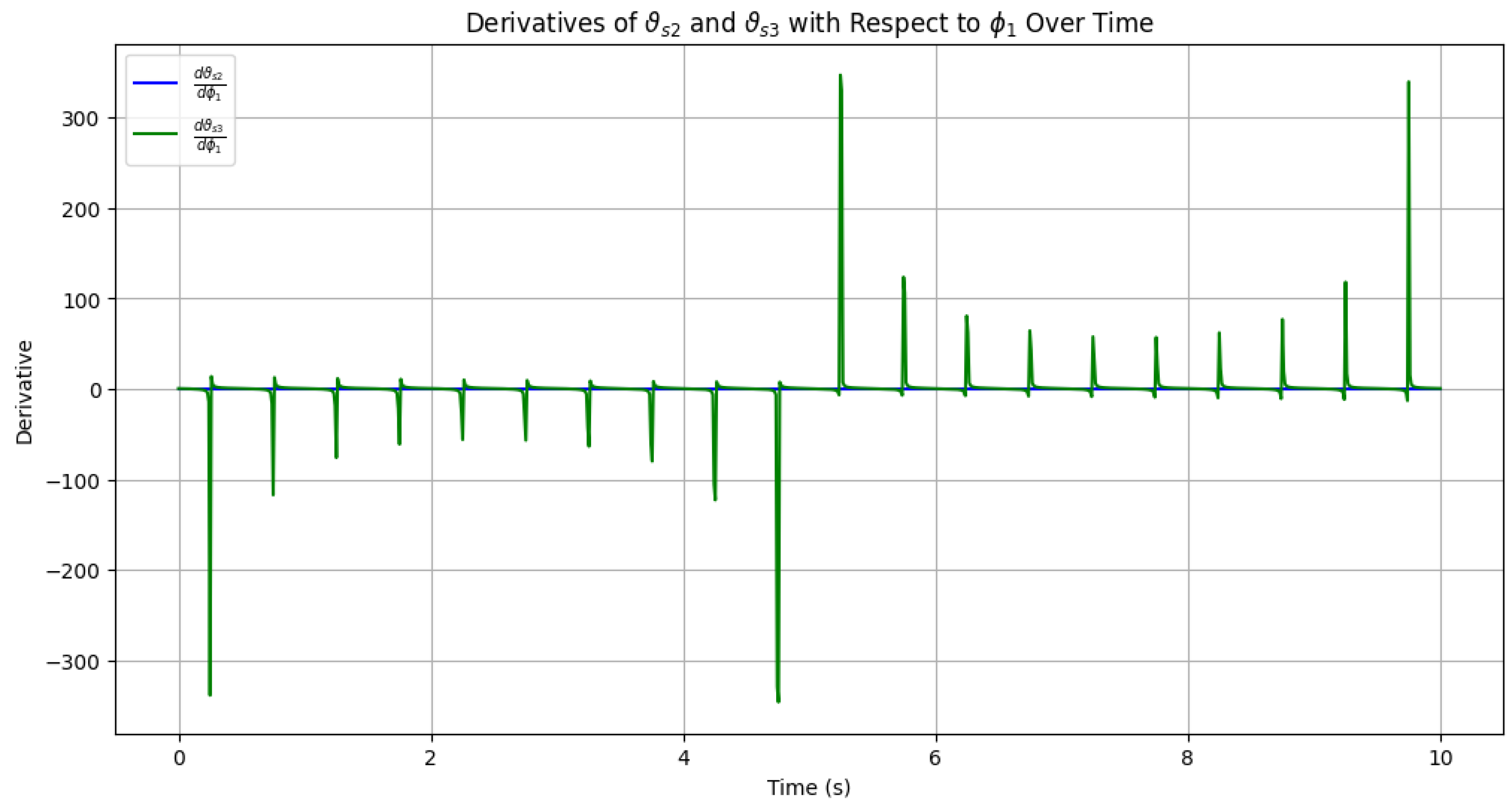
  • Kinematic analysis. The kinematic analysis focused on describing the motion of the system’s components without considering the forces or torques causing the motion: a) System modeling - the conveyor mechanism was modeled as a system of interconnected rigid links with specified lengths ( L 1 , L 2 ,…) and joints. Angular displacements ( φ 1 ,   φ 2 , ) were used to describe the positions of the links relative to reference points. b) Geometric and trigonometric relationships - constraints between the links were expressed as equations involving sines and cosines of the angular variables. Relationships such as L 1 c o s φ 1 + L 2 c o s φ 2 = L 3 c o s φ 3 were used to ensure consistency in the system’s geometry. c) Velocities and accelerations - the angular velocities and angular accelerations were derived using time differentiation of the position equations. The motion constraints were used to compute velocities and accelerations for all components. d) Visualization - 3D plots of angular displacement, velocity, and acceleration were generated to illustrate the motion behavior over time.
  • Dynamic analysis. The dynamic analysis incorporated the forces and torques acting on the system to evaluate its response under load. a) Derivation of equations of motion - Newton’s Second Law and the principle of virtual work were applied to derive equations governing the system’s dynamics. Inertia terms I φ i were computed using the mass distribution and geometry of the system. b) Force and torque calculations - driving torques M d and resisting torques M r were modeled as functions of angular velocity ω 1 and angular displacement φ 6 . External factors, such as damping and load resistance, were incorporated into the dynamic equations. c) Nonlinear effects - nonlinear terms, such as those involving products of angular velocities and displacements, were explicitly included to account for real-world interactions. d) System stability - stability conditions were analyzed by evaluating the balance of forces and torques during operation. Parameters like stiffness K and base moments M r 0 were studied to ensure system stability.
  • Numerical approximation. The numerical approximation was used to solve the nonlinear differential equations derived in the dynamic analysis. a) Differential equation formulation - the equations were expressed in the standard form:
    R ( t ) d ω 1 d t + Q ( t ) ω 2 ( t ) = W ( t )
    where R t ,   Q ( t ) , and W ( t ) are time-dependent coefficients. b) Discretization - Euler’s method was employed to approximate the derivatives using finite time steps h:
    ω k + 1 = ω k + h W k R k Q k R k ω k 2
    angular displacement was updated iteratively:
    φ k + 1 = φ k + h ω k
c) Initial conditions - Initial values for angular displacement φ 1 = 0 and angular velocity ω 1 = 0 were specified at t=0. d) Simulation - Time was discretized into intervals, and the system’s behavior was computed step by step. Parameters such as A ( t ) , B(t), D(t), E(t), F(t), H ( t ) , N(t), M(t), Q ( t ) , R t , and W ( t ) were evaluated at each time step. E) Validation and visualization - the numerical results were compared with theoretical expectations to ensure accuracy. Time-series and 3D plots of dynamic variables were generated for visualization. Due to the complexity of the equation, analytical solutions are impractical. Numerical integration (Runge-Kutta method) was employed, allowing for accurate computation of the time evolution of φ 1 t and ω 1 t . For each time step, we iteratively calculate the angular velocity ω k and the angular position φ k . The total simulation time is divided into N steps, and the time step h determines the accuracy of the approximation. Initial conditions are specified at t=0: ω 0 = 0 and φ 0 = 0 . The equation of motion is discretized using the Euler method, leading to the iterative formulas for ω k + 1 and φ k + 1 . Stability of the solution depends on the choice of step size h, with smaller values yielding more accurate results at the cost of increased computational time. The accuracy of the method is first-order, meaning the error decreases quadratically with the step size h. The computational efficiency is an important consideration, especially if the system is large or requires many time steps.

4. Results

This section may be divided by subheadings. It should provide a concise and precise description of the experimental results, their interpretation, as well as the experimental conclusions that can be drawn. To compute the exact derivatives of ϑ S 2 and ϑ S 3 with respect to φ 1 over time, you need to express these variables in terms of φ 1 and its time-dependent behavior show in Figure 4. After that, we use the differentiation rules and chain rules to find time derivatives, including any relationships between angular velocity or other relevant parameters in the system. To plot the derivatives of u 21 and u 51 with respect to φ 1 (i.e., d u 21 d φ 1 and d u 51 d φ 1 ), we need the expressions for u 21 and u 51 in terms of φ 1 show in Figure 5. We can compute the derivatives of these expressions with respect to φ 1 and then plot them.
M d t = s i n ω 1 e 0.1 t A damped sinusoidal function. M r t = c o s φ 6 × 1 + 0.5 s i n t A modulated cosine function. Below are 3D plots for M d t as a function of ω 1 and M r t as a function of φ 6 . These assume some general functional forms for M d t and M r t , but they can be replaced with specific equations or data show in Figure 6. To analyze the 3D graphs below, it is first necessary to understand their physical meaning and how they change with time, angular velocity ( ω 1 ), and angular position ( φ 6 ). In this graph, the torque M d t is plotted as a function of time and angular velocity (ω1). The function sin( ω 1 ) produces sinusoidal oscillations with respect to ω 1 , indicating that the torque varies cyclically. exp(−0.1t) as time t increases, the amplitude of the torque decreases, indicating the damping or damping effect. Initially, the amplitude of the M d is maximum and decreases with time. This is explained by the energy loss in the kinematic system (e.g., due to friction). At high values of ω 1 , the amplitude of the oscillations changes little, but the frequency increases. This graph is useful for predicting the change in torque, adjusting the damping parameters, and studying the stability of the system. The second graph shows the torque M r t as a function of time and angular position ( φ 6 ). cos( φ 6 ) M r t varies sinusoidally with angular position. This indicates several complete cycles over a certain period of time. (1+0.5sin(t)) the amplitude of the torque is modulated with time t. That is, the vibration level changes with time. The dependence on φ 6 indicates the cyclical nature of the vibration, which indicates the uniformity or repetition of the rotational motion in the mechanism. The dependence on t leads to an increase or decrease in the amplitude at a certain time, which indicates the sensitivity of the rotating system to external influences. This graph allows us to assess the stability of M r t with respect to angular position and time. It is useful for studying the phase balance and dynamics of the device over time.
The resulting 3D graphs from the Python provide insights into the oscillatory behaviors of the variables over time. Here’s an analysis of each graph: A(t) exhibits sinusoidal oscillations whose amplitude gradually decreases over time due to exponential damping (exp(−0.1t)) show in Figure 7. B(t) is a cosine wave with slower exponential decay (exp(−0.05t)) compared to A(t) show in Figure 7. Useful for systems with slower energy dissipation, such as lightly damped mechanical systems. D(t) A sinusoidal wave superimposed on a linear increasing trend (2t) show in Figure 8. Represents oscillatory systems influenced by a steady growth, such as systems with a baseline drift. E(t) Superposition of two sinusoidal waves with different frequencies leads to a complex pattern, showing periodic reinforcement and cancellation (beat phenomena). Common in wave interference, acoustics, or alternating currents with multiple harmonics show in Figure 8. F(t) The product creates a modulated waveform with periodic variations in amplitude show in Figure 9. Found in amplitude-modulated (AM) signals in communication systems. H(t) Sinusoidal oscillations where the amplitude grows quadratically with time (0.5t2). Useful in modeling systems where oscillatory behavior becomes increasingly intense, such as resonant systems show in Figure 9 (average around 1.0215 with oscillations ±0.1). N(t) A simple sine wave with a fixed frequency and amplitude show in Figure 10. Idealized representation of pure harmonic motion. M(t) Similar to N(t), but with a phase shift of π/2. Complements N(t) in systems requiring orthogonal oscillations show in Figure 10, such as in-phase and quadrature components. Q(t) High-frequency oscillation with a small amplitude show in Figure 11. Models small perturbations or noise-like oscillatory components in systems. R(t) Oscillatory behavior with a baseline offset (5+…) show in Figure 11. Represents resistive fluctuations in electrical or mechanical systems with a steady mean resistance. W(t) A pure sine wave driving force (ranges from 1.8 to 2.2, periodic fluctuations add variability). This type of behavior is typical for systems subject to periodic forcing, such as driven pendulums or AC circuits show in Figure 12.

5. Discussion

The presented differential equation governing the movement of the oscillating conveyor mechanism provides a comprehensive model for analyzing the system’s dynamic behavior over time. This model incorporates various parameters related to the mechanical system, such as resisting torque ( M r ), driving torque ( M d ), inertial moments ( I S 1 , I S 2 , I S F , I 6 G ), and dynamic terms involving angular displacements ( φ 1 , φ 2 , etc.), angular velocities ( ω 1 , ω 2 , ω 6 ), and their corresponding time derivatives. The equation captures the interactions between the resistive and driving forces in the system and how these forces influence the motion of the mechanism. The system is subject to a variety of forces that are modeled through functions like A(t), H(t), Q(t), and W(t), which depend on the time-varying nature of the system’s geometry, velocity, and other dynamic variables. Notably, the resistive torque M r is modeled as a linear function of φ 6 , reflecting the physical behavior of the resisting torque as the angular position changes. Similarly, the driving torque M d is affected by a damping term proportional to ω 1 , which accounts for frictional or resistive losses in the system. These dynamic interactions influence the evolution of angular velocities and positions over time. The equation is solved using an approximate method, specifically an explicit finite difference approach, where the angular velocity ω and angular displacement φ are computed at discrete time steps. This numerical integration method enables the prediction of system behavior over time based on initial conditions. The time step h and total simulation time T are key factors that influence the accuracy of the numerical solution. In this case, an initial angular displacement of φ 0 = 0 and initial angular velocity ω 0 = 0 are used as starting conditions, and the system is modeled over the interval [0, T]. By iterating through the algorithm at each time step, we can track the evolution of angular velocities and displacements, providing insight into the system’s stability and response to various forces. This approach is particularly useful for studying complex systems like oscillating conveyors [17], where analytical solutions are difficult to derive.
Key Observations:
System damping - the model’s inclusion of damping in the form of α (a damping coefficient) highlights the importance of frictional forces in the system’s behavior. The damping term, which is proportional to angular velocity ω 1 , plays a significant role in regulating the amplitude of oscillations over time. This is crucial in understanding how the conveyor mechanism stabilizes and the rate at which it dissipates energy.
Nonlinear dynamics - the nonlinear relationship between the angular velocities and torques, particularly in the form of ω2 terms and the dependency of R(t) and Q(t) on time-varying functions, reflects the complex nature of the system’s dynamics. These nonlinearities must be carefully accounted for when analyzing the system’s behavior, especially in cases where large displacements or velocities occur.
Sensitivity to initial conditions - the system’s sensitivity to initial conditions, such as the starting angular displacement and velocity, indicates the importance of accurate measurements and control in real-world applications. The behavior of the system may vary significantly depending on the initial conditions, which highlights the need for precise calibration in practical implementations.
Numerical stability and accuracy - the choice of time step h is crucial for the stability and accuracy of the numerical solution. A smaller h improves accuracy but increases computational effort, while a larger h may lead to numerical instability or inaccuracies. Thus, balancing computational efficiency with accuracy is an essential consideration when solving this type of differential equation.
Future work - to improve the model’s realism and applicability, further work could involve incorporating more detailed effects such as non-constant damping coefficients, elastic deformations of the conveyor components, or external disturbances like loading variations. Additionally, real-time measurements and feedback control strategies could be integrated to optimize the conveyor’s performance and mitigate issues such as resonance or instability. By extending this model to include more components or refining the numerical methods used, the system could be better suited for practical implementation in vibration conveyors or similar systems.

6. Conclusions

The kinematic analysis of the vibration conveyor mechanism provided insights into the motion of its components, including their positions, velocities, and accelerations. By modeling the geometric and trigonometric relationships between the links, the study established how the angular displacements, velocities, and accelerations evolve over time. The analysis highlighted the importance of understanding the interplay between link lengths, joint angles, and motion constraints for optimizing the mechanism’s design and ensuring smooth operation. The results can be used to predict motion trajectories and to ensure that the conveyor operates within its intended range of motion, minimizing the risk of mechanical interference or instability. Dynamic analysis revealed the forces and torques acting on the vibration conveyor system, accounting for inertia, damping, and external forces. The study demonstrated how the system responds to dynamic loads and how these forces influence the stability and efficiency of the mechanism. The derived equations of motion captured the nonlinear interactions between the system’s components, including the effects of centrifugal and inertial forces. By quantifying these forces, the analysis enabled the identification of optimal operating conditions and highlighted the need for proper force balancing and damping to minimize vibrations and wear. The numerical approximation provided a practical method for solving the nonlinear differential equations governing the vibration conveyor mechanism. Methods such as Euler’s method and the Runge-Kutta approach allowed for accurate simulations of the system’s behavior over time. These techniques enabled the visualization of time-dependent variables, such as angular velocity and system forces, under varying conditions. The numerical results closely matched the expected theoretical outcomes, validating the mathematical model and the approximations used. This approach is particularly valuable when exact analytical solutions are intractable, offering a reliable way to simulate and analyze complex dynamic systems. The combination of kinematic analysis, dynamic analysis, and numerical approximation provides a comprehensive understanding of the vibration conveyor mechanism. This multi-faceted approach facilitates: Insights into motion and force interactions enable improved designs for efficiency and reliability. By simulating system responses under various conditions, potential failure modes can be identified early. Accurate modeling supports fine-tuning of operational parameters to achieve desired performance. The methodologies and results from this study can be extended to similar mechanisms, laying the foundation for robust mechanical system analysis and design in industrial applications.

Author Contributions

Conceptualisation, A.Z.; methodology, A.Z.; software, A.Z.; validation, A.Z.; formal analysis, A.Z. and K.A; investigation, A.Z.; resources, A.A. and G.B.; data curation, A.O.; writing—original draft preparation, A.Z., G.B. and K.A.; writing—review and editing, A.Z., A.A. and A.O.; visualisation, A.Z. and A.O.; supervision, A.Z.; project administration, A.Z. and A.A.; funding acquisition, A.Z., G.B. and K.A.; All authors have read and agreed to the published version of the manuscript.

Funding

This research was funded by Almaty University of Power Engineering and Telecommunications named after Gumarbek Daukeyev, grant number AP19677356.

Institutional Review Board Statement

The study did not require ethical approval.

Informed Consent Statement

Not applicable.

Data Availability Statement

Data are contained within the article.

Acknowledgements

This work has been supported financially by the research project (AP19677356 - To develop systems for controlling the orientation of nanosatellites with flywheels as executive bodies based on linearization methods) of the Ministry of Education and Science of the Republic of Kazakhstan and was performed at Research Institute of Communications and Aerospace Engineering in Almaty University of Power Engineering and Telecommunications named after Gumarbek Daukeyev, which is gratefully acknowledged by the authors.

Conflicts of Interest

The authors confirm that they have no conflict of interest with respect to the work described in this manuscript.

References

  1. Gurskyi, V.; Korendiy, V.; Krot, P.; Dyshev, O. Determination of kinematic and dynamic characteristics of a reversible vibratory conveyor with an electromagnetic drive. Vibroengineering Procedia 2024, 55, 138-144. [CrossRef]
  2. Korendiy, V.; Kachur, O.; Dmyterko, P. Kinematic analysis of an oscillatory system of a shaking conveyor-separator. Advanced Manufacturing Processes III 2022, 592-601. [CrossRef]
  3. Gurskyi, V.; Korendiy, V.; Krot, P.; Zimroz, R.; Kachur, O.; Maherus, N. On the dynamics of an enhanced coaxial inertial exciter for vibratory machines. Machines 2023, 11, 97. [CrossRef]
  4. Shah, K.P. Construction, working and maintenance of electric vibrators and vibrating screens. Available online: https://practicalmaintenance.net/wp-content/uploads/Construction-Working-and-Maintenance-of-Vibrators-and-Vibrating-Screens.pdf (accessed on 8 December 2022).
  5. Cieplok, G.; Wójcik, K. Conditions for self-synchronization of inertial vibrators of vibratory conveyors in general motion. J. Theor. Appl. Mech. 2020, 58, 513–524. [CrossRef]
  6. Nguyen, V.X.; Nguyen, K.L.; Dinh, G.N. Study of the dynamics and analysis of the effect of the position of the vibration motor to the oscillation of vibrating screen. J. Phys. Conf. Ser. 2019, 1384, 012035. [CrossRef]
  7. Nazarenko, I.; Gaidaichuk, V.; Dedov, O.; Diachenko, O. Investigation of vibration machine movement with a multimode oscillation spectrum. East.-Eur. J. Enterp. Technol. 2017, 6, 28–36. [CrossRef]
  8. Chen, Z.; Tong, X.; Li, Z. Numerical investigation on the sieving performance of elliptical vibrating screen. Processes 2020, 8, 1151. [CrossRef]
  9. Gursky, V.; Krot, P.; Korendiy, V.; Zimroz, R. Dynamic analysis of an enhanced multi-frequency inertial exciter for industrial vibrating machines. Machines 2022, 10, 130. [CrossRef]
  10. Gursky, V.; Kuzio, I.; Krot, P.; Zimroz, R. Energy-saving inertial drive for dual-frequency excitation of vibrating machines. Energies 2021, 14, 71. [CrossRef]
  11. Yaroshevich, N.; Puts, V.; Yaroshevich, Т.; Herasymchuk, O. Slow oscillations in systems with inertial vibration exciters. Vibroengineering Procedia 2020, 32, 20–25. [CrossRef]
  12. Yaroshevich, N.; Yaroshevych, O.; Lyshuk, V. Drive dynamics of vibratory machines with inertia excitation. In Vibration Engineering and Technology of Machinery; Balthazar, J.M., Ed.; Springer International Publishing: Cham, Switzerland, 2021; pp. 37–47.
  13. Chen, B.; Yan, J.; Yin, Z.; Tamma, K. A new study on dynamic adjustment of vibration direction angle for dual-motor-driven vibrating screen. Proc. Inst. Mech. Eng. Part E J. Process Mech. Eng. 2021, 235, 186–196. [CrossRef]
  14. Cieplok, G. Verification of the nomogram for amplitude determination of resonance vibrations in the run-down phase of a vibratory machine. Journal of Theoretical and Applied Mechanics 2009, 47, 2, 295-306.
  15. Michalczyk, J.; Cieplok, G. Disturbances in self-synchronisation of vibrators in vibratory machines. Archives of Mining Sciences 2014, 59, 1, 225-237. [CrossRef]
  16. Zhao, C.; Zhao, Q.; Gong, Z.; Wen, B. Synchronization of two self-synchronous vibrating machines on an isolation frame. Shock and Vibration 2011, 55, 1-2, 73-90.
  17. Zhauyt, A. The substantiating of the dynamic parameters of the shaking conveyor mechanism. Vibroengineering Procedia 2015, 5, 15-20.
  18. Wyk, J., Snyman, A., Heyns, S. Optimization of a vibratory conveyor for reduced support reaction force. N&O Journal 1994, 1(10), 12-17.
  19. Andrea, V.; Nicolae, U.; Loana, M. Contribution to the optimization of relative motion on a vibrating conveyor. ACTA Technica Napocensis 2012, 2(55), 519-522.
  20. Chu, Yiqing; Li, Cuiying. Helical vibratory conveyors for bulk materials. Bulk Solid Handling 1987, 1(7), 103-112.
  21. Sloot, E.M.; N.P. Kruyt, N.P. Theoretical and experimental study of the conveyance of granular materials by inclined vibratory conveyors. Powder Technology 1996, 87(3), 203-210.
  22. Despotovic, Z.; Stojiljkovic, Z. A realization AC/DC transistor power converter for driving electromagnetic vibratory conveyors. Proc. of the V Symp. of Indu. Elec. INDEL, Banja Luka, 11-13.IX.2004, T2A, 34-40.
  23. Despotovic, Z.; Stojiljkovic, Z. Power converter control circuits for two-mass vibratory conveying system with electromagnetic drive: simulations and experimental results. IEEE Transation on Industrial Electronics 2007, 54(I), 453-466. [CrossRef]
  24. Winkler, G. Analysing the vibrating conveyor. International Journal of Mechanics 1978, 20, 561-570.
Figure 1. Kinematical schema of the three-class mechanism.
Preprints 146024 g001
Figure 2. Kinematic scheme of the mechanism relative to the center of gravity.
Preprints 146024 g002
Figure 3. The first subplot shows the relationship between M r and φ 6 . The second subplot shows the relationship between M d and ω 1 .
Preprints 146024 g003
Figure 4. Derivatives of ϑ S 2 and ϑ S 3 with respect to φ 1 over time.
Preprints 146024 g004
Figure 5. Derivatives of u 21 and u 51 with respect to φ 1 over time.
Preprints 146024 g005
Figure 6. 3D plots are given for M d ( t ) as a function of ω 1 and M r ( t ) as a function of φ 6 .
Preprints 146024 g006
Figure 7. A grid of 3D plots showing the behavior of A(t) and B(t).
Preprints 146024 g007
Figure 8. A grid of 3D plots showing the behavior of D(t) and E(t).
Preprints 146024 g008
Figure 9. A grid of 3D plots showing the behavior of F(t) and H(t).
Preprints 146024 g009
Figure 10. A grid of 3D plots showing the behavior of N(t) and M(t).
Preprints 146024 g010
Figure 11. A grid of 3D plots showing the behavior of Q(t) and R(t).
Preprints 146024 g011
Figure 12. A grid of 3D plots showing the behavior of W(t).
Preprints 146024 g012
Table 1. A tabular representation of the steps and their descriptions.
Step Description
Inputs Inputs: ω 0 , φ 0 , N, h
Increment n Set n: = n+1
Compute A(tn) Compute A(tn)
Compute B(tn) Compute B(tn)
Compute D(tn) Compute D(tn)
Compute E(tn) Compute E(tn)
Compute F(tn) Compute F(tn)
Compute H(tn) Compute H(tn)
Compute N(tn) Compute N(tn)
Compute M(tn) Compute M(tn)
Compute Q(tn) Compute Q(tn)
Compute R(tn) Compute R(tn)
Compute W(tn) Compute W(tn)
Update ω n + 1 ω n + 1 = ω n + h (Wn/Rn-Qn/Rn * ω n )
Update φ n + 1 φ n + 1 = φ n   + h ω n
Check if n < N Check if n < N
Yes: Update ω n ,   φ n and Repeat If ‘Yes’, Update ω n ω n + 1 , φ n φ n + 1 and Repeat
No: Output ω n + 1 , φ n + 1 If ‘No’, Output final ω n + 1 , φ n + 1
End End of process
Disclaimer/Publisher’s Note: The statements, opinions and data contained in all publications are solely those of the individual author(s) and contributor(s) and not of MDPI and/or the editor(s). MDPI and/or the editor(s) disclaim responsibility for any injury to people or property resulting from any ideas, methods, instructions or products referred to in the content.
Copyright: This open access article is published under a Creative Commons CC BY 4.0 license, which permit the free download, distribution, and reuse, provided that the author and preprint are cited in any reuse.
Prerpints.org logo

Preprints.org is a free preprint server supported by MDPI in Basel, Switzerland.

Subscribe

Disclaimer

Terms of Use

Privacy Policy

Privacy Settings

© 2025 MDPI (Basel, Switzerland) unless otherwise stated