Submitted:
16 January 2025
Posted:
20 January 2025
Read the latest preprint version here
Abstract
We developed a web application demo, dynamically monitoring and visualizing the traffic condition in New York City, with a focus on Manhattan. We took advantage of two public API providers: tomtom and openweather, to request traffic-related streaming data including real-time intersection speed, historical density, and weather details. We acquired speed data every 15 minutes, weather data once an hour, density once a day, and updated the traffic heatmap every 15 minutes. We implemented our visualization by Google Maps APIs and similar to Google Map layout, we quantified the congestion into three degrees and plotted streets with colors. Our web demo achieved similar performance with Google Maps, but with more reasonable and accurate results. Our work can also accept streaming data to achieve high-level concurrency.
Keywords:
Real-time Visualization
; Async Streaming
; Traffic Analysis
1. Problem Declaration
It is struggling to drive in Metropolitan, as in a crowded city, vehicles and pedestrians are everywhere. In this case, road conditions are likely to be complicated. Moreover, if there is a temporary event, for instance, road closure or traffic accident, traffic will definitely be in chaos. Take New York City as an example. There are more than 14k roads of all levels, needless to say intersections. Roads are planned and constructed in grid-like manner, with orthogonal and parallel layout. If you want to travel from one place to another, even though they are not far away from each other, there are still multiple available routes. So instead of locating the shortest route, it is more necessary to find the quickest one under continuously changing traffic.
We have investigated several publications and open-sourced codes. [3] merely focused on visualization based on processed data; [4] conducted analysis with logistic regression. We not only worked on visualization on Google Map, but did more sophisticated investigations on the analysis with more than free-flow speed. [5] transformed roads and intersections into connected graph and developed topology model for traffic congestion prediction. The basic formula is the product of traffic density and traffic speed. While we also leveraged the formula as the analysis principle, we did not have access to the video data and traffic light policy that the paper heavily counted on. As for successful commercial tools, one of examples is Google Map. The core idea behind such a strong tool is that it relies on user feedback. Unfortunately, human judgements are not always precise, and there is always deviation from the real-world observation.
Based on the preliminary investigations, we narrowed our problem into two main challenges: data acquisition and model correction. As we didn’t have access to videos from city surveillance cameras, we sought for alternatives. The demand of the data should be streaming, as we planned to build real-time heatmap. Also, given thousands of streets and intersections within such a crowded area as our first practice, data also needs to be dense and precise, especially when it comes to geographic locations. Among all available tools, [1] developer has strong interfaces for accessing both real-time and historical data. Also, we need to count on real-time weather to correct the analysis model. Besides weather impact, there are also other external factors, to illustrate, emergent road closure, car crash and special event. We also highlighted these areas to alert drivers. The implementation details will be discussed thoroughly in the following chapters.
2. Methodology
2.1. System Architecture Overview
The system architecture is shown in Figure 1. The whole structure can be divided into three core components, data processing with [6], analysis model with Python, and visualization with Flask and MySQL. We name these components as data processing, congestion model and visualization for simplicity in the following subsections.
Everything starts with a file set named centerline. This is extracted from [7] with all road details in New York City. Given a huge amount of data and enormous repetition, the roads were downsampled to an acceptable quantity. These road information is the official input of the whole structure. There are two branches to process these roads. One is served as the request parameters in [1] traffic flow API call, another is used for [2] One Call. We obtained traffic speed and weather information responses from the two calls. These responses will be flowed into the evaluation model. Another critical input of the evaluation model is the traffic density. Given that it is region-based historical data, we can prepare it without explicit geographic coordinates. We roughly separate Manhattan into 24 local regions based on community, and we navigate a specific road density in a hierarchical manner. First we direct the road to the nearest region center, and after that the road will be matched to the nearest segment in the local region with traffic density information. The output of the evaluation model is the traffic congestion score. These scores will be stored in MySQL database with current time as table name. Whenever there is a fresh or a trigger, these scores will be extracted from the Flask and visualized with HTML, CSS, JavaScript developer toolkit on Google Maps Platform.
2.2. Data Processing
Data processing is developed under [6] and Spark Streaming. The static data (road coordinates) was processed by [6] and streaming data was processed by Spark Streaming.
2.2.1. Static Data Processing
Static data processing happened when points and calls are fast to obtain and not huge in quantity. In the raw street file provided by [7], there are more than 140,000 road segements. We firstly get rid of repetitive street annotations, with more than 90% of roads were excluded. After that, we restricted the region in Manhattan only by filtering zip code. Ultimately we had 1,000 records as input of the analysis and visualization model. Given less than 10,000 points to call, we could easily store everything in one file. You could either read the points into Spark DataFrame or Spark RDD.
Spark data would be sent through two branches, traffic speed acquisition and real-time weather acquirement. Points could be sent as request parameters in forEach loop. For traffic speed, there is a huge diversity amongst intersections, as it internally may have something to do with road infrastructure design (number of lanes), and speed limit, externally is relevant to emergent situations like road closure and restrictions. So there was no downsampling strategy of traffic speed call. However, when it comes to weather API call, things became completely different. Unlike continuously fluctuated traffic conditions, weather is more likely to remain immutable within a specific region at a time spot. In this case, we implemented clustering to divide Manhattan into 8 regions with K-Means. We only needed to call the weather at the cluster centroids to represent the local weather of that region.
As the points were fixed, we had a fixed number of calls during each trigger. We concatenated each functional API response as a list of RDDs and set them as inputs of evaluation model.
2.2.2. Streaming Data Processing
Whenever there is an update on the Map or we intend to expand our view outside New York City, we may want streaming input. The major difference between streaming and static data processing is that when the data is static, we only downsampled and transformed it once. Same process would always be applied in subsequent processes. But when the data was streaming data, we needed to downsample and transform each batch of streaming data. Suppose we had multiple different text files for storing street records and a new text file would be generated at some intervals. The program would always include updated points. As for API calls, we could build a queueStream with new response appended at the rear of the queue. Figure 2 shows the flow of our streaming processing in this case.
textFileStream could create an data stream monitoring for new text files storing street records and then loads them. The filtering and deduplication strategy is the same as static method.
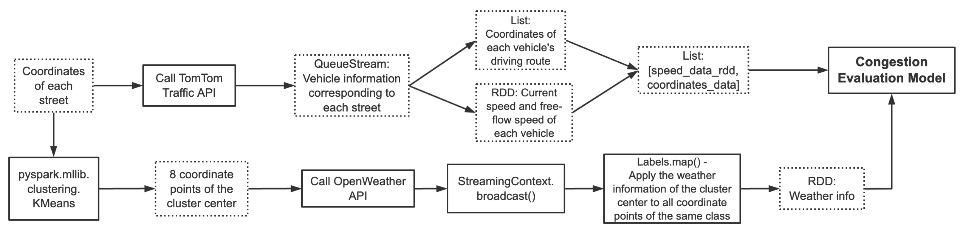
Upon getting the vehicle information corresponding to each street through the [1] Traffic API, we stored the coordinates of each vehicle’s driving route as a coordinate queue, and at the same time stored the driving speed and free-flow speed of each vehicle as an RDD. Finally we merged the two into a list. We also continuously updated the cluster centers with new streaming points to get weather details, and broadcast it to all intra-points. Then we transferred processed vehicle trajectories and weather data into the congestion evaluation model for subsequent calculations. Figure 3 shows the detailed processing flow.
2.2.3. Streaming Algorithm
Once we have the streaming data as input, it is likely that we need to deal with large amount of data. As we are developing a real-time traffic heatmap, we have strict demand of processing latency. During the development, we found that the most time-comsuming step is the API calls, especially the [1] traffic flow APIs as we needed to call them more than 1,000 thousand times per 15 minutes. For each API call, it consists of overhead for session establishment and request/response for GET/POST request. The first optimization we could implement is to reduce overhead cost by keeping alive a session all the time. This will avoid establishing a session for every API call.
Also we found that all points are independent with each other and API calls are only related to the requested points themselves. We regarded the API calls as stateless operations and the further improvement was to have asynchronized API calls. Figure 4 shows the time series execution logic. We have two third-party packages to implement this: asyncio and aiohttp. The former one is used to set up co-routine and achieve high-level of concurrency, and the latter one is served as a middleware in the web-server. There are two keywords of triggering asynchronous call: async and await, where first one is the signal of activating a co-routine and the second one is a signal of interruption of executing the asynchronous program.
Figure 4.
async API Call
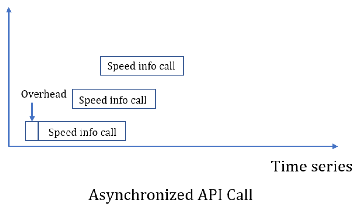
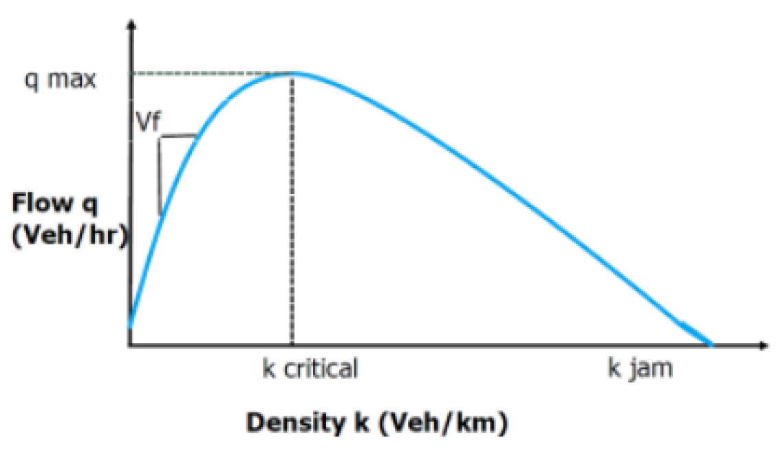
Figure 5.
Fundamental traffic flow curve
If we reviewed our backend module in a system-level prospective, we could optimize the streaming data processing with FAIR scheduler. The program would be executed in a FIFO manner by default. If two significantly different and stateless tasks with different resource and time consumption expectation were executed sequentially and difficult job started first, it is likely that the job would take up all the computing resources. And the easy job would be executed only after the difficult job was completed. FAIR scheduler will avoid such a situation by properly allocating resources to all jobs. In Apache Spark, each job is called a pool, separating resources of different clients. We used weight to set up job priority and minShare to avoid the scheduler being downgraded into FIFO manner.
2.3. Congestion Model
We observe traffic congestion is inversely proportion to traffic flow, presented in equation 1.
We learnt that using traffic density to determine traffic congestion is tricky. If the traffic density is too high, the scenario may be vehicles are travelling on express highway where there is less traffic light. Or if the traffic density is too low, the scenario may turn out to be travelling in the midnight where there are few cars on the streets. Figure 5 shows the basic curve of traffic flow with respect to traffic density.
Based on the specialization of traffic flow, we correct our evaluation model by having small punishment with high and low traffic density. We also evaluate the speed deviation with L2 distance, along with weather impact. All weather coefficients are emperical, extract from [8]. Also, we found there was a scaling difference between speed deviation and density punishment, but we considered both factors should have equal contributions to the evaluation of traffic congestion. The ultimate evaluation formula is shown in equation 2.
Figure 6.
Visualization screenshot
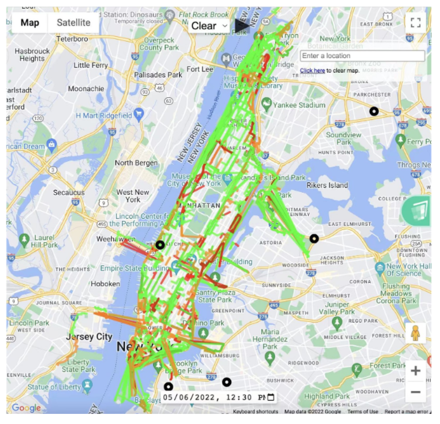
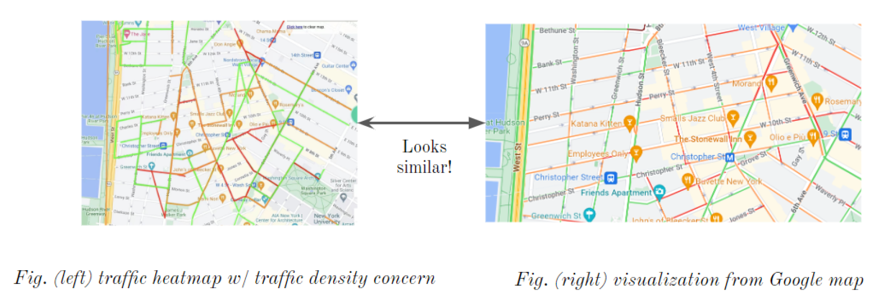
Figure 7.
Evaluation comparison
2.4. Visualization
The visualization was built on [9]. We mainly focused on Maps JavaScripts API and roads API. Our evaluation results include segment coordinates, weathers and congestion scores. We quantized the scores with two threshold: -100 and -500, and indicated three degrees: no congestion (green), slight congestion (orange) and heavy congestion (red). The visualization also include alert of historical car crash incidents as black dots. Except real-time traffic heatmap visualization, we supported playback of past 24-hour traffic condition change and navigation back to the latest traffic condition given a specific weather. We now support rainy, snowy, foggy and tornado playback. The screenshot is shown in Figure 6.
To evaluate our visualization, we select west side of Manhattan downtown, a dense area with tens of intersections at 8 pm, May 5th. We compared our result with Google Map. In Figure 7, we found that the visualization is similar in coloring, meaning our evaluation is somehow reasonable.
There are two major difficulties during implementation, one is the visualized data needs to be post-processed before being read by JavaScript for data format and precision adjustment. We used Flask to build a middleware between the MySQL cursor and JavaScript. Frontend will send a POST or GET request through Flask, the cursor will fetch corresponding data from MySQL. Second is that the route drawing response is slow and inefficient with large quantity of data. To avoid an awkward situation where the map was not filled, we found that there is no need to clear the map every time before the traffic congestion was updated. Instead, we can keep the old traffic condition visualization and draw lines on top of the old lines. Once the update is completed, we can clear the old visualizations.
3. Review and Future Work
We developed a web application upon Google Maps Platform. As we developed our demo with limited time, there is still room for improvement. Based on the feedback from the presentation, we concentrate our future work to three issues:
We may deploy our application to cloud servers to support multi-user access. We can upload our program to Google Cloud Platform. We can store our data in BigQuery and set our scheduler via Airflow, with program triggered every 15 minutes.
We may expand our heatmap to route recommendations. We can leverage Google Maps Direction API to present candidate routes from one place to another and combine our heatmap to determine the fastest route. Besides, we can leverage the current speed from [1] API to calculate expected commuting time.
We may leverage window function to smooth our playback. We can set up a time interval as window and slide the window to exclude older data and accept newer data and the playback can be smoothed from GIFs to videos.
Acknowledgments
This work is the final project of course ELEN-6889 Large-scale Stream Processing, instructed by Professor Deepak S. Turaga. We thank him for his help with this report and all the feedbacks for the proposal and demonstration presentation.
References
- Tomtom. tomtom. [EB/OL], 2022. https://developer.tomtom.com/ Accessed May 8, 2022.
- openweather. openweather. [EB/OL], 2022. https://openweathermap.org/api Accessed May 8, 2022.
- pranathim1. Real-time-visualization-of-NYC-Traffic-data. [EB/OL], 2017. https://github.com/pranathim1/Real-Time-Visualization-of-NYC-Traffic-Data Accessed Mar. 3, 2017.
- xiaotongxin. Spark-Streaming-TrafficJamPrediction. [EB/OL], 2019. https://github.com/xtxxtxxtx/SparkStreaming-TrafficJamPrediction Accessed Aug. 23, 2019.
- Abbas, Z.; Sottovia, P.; Hajj Hassan, M.A.; Foroni, D.; Bortoli, S. Real-time Traffic Jam Detection and Congestion Reduction Using Streaming Graph Analytics. In Proceedings of the 2020 IEEE International Conference on Big Data (Big Data), 2020, pp. 3109–3118. [CrossRef]
- Spark, A. Spark. [EB/OL], 2022. https://spark.apache.org/docs/latest/index.html Accessed May 8, 2022.
- OpenData, N. nyc opendata. [EB/OL], 2022. https://opendata.cityofnewyork.us/ Accessed May 8, 2022.
- Hani S. Mahmassani, Jing Dong, J.K.; Chen, R.B. Incorporating Weather Impacts in Traffic Estimation and Prediction Systems. [EB/OL], 2009. https://rosap.ntl.bts.gov/view/dot/3990.
- maps platform. maps platform. [EB/OL], 2022. https://developers.google.com/maps/documentation Accessed May 8, 2022.
Figure 1.
System Architecture
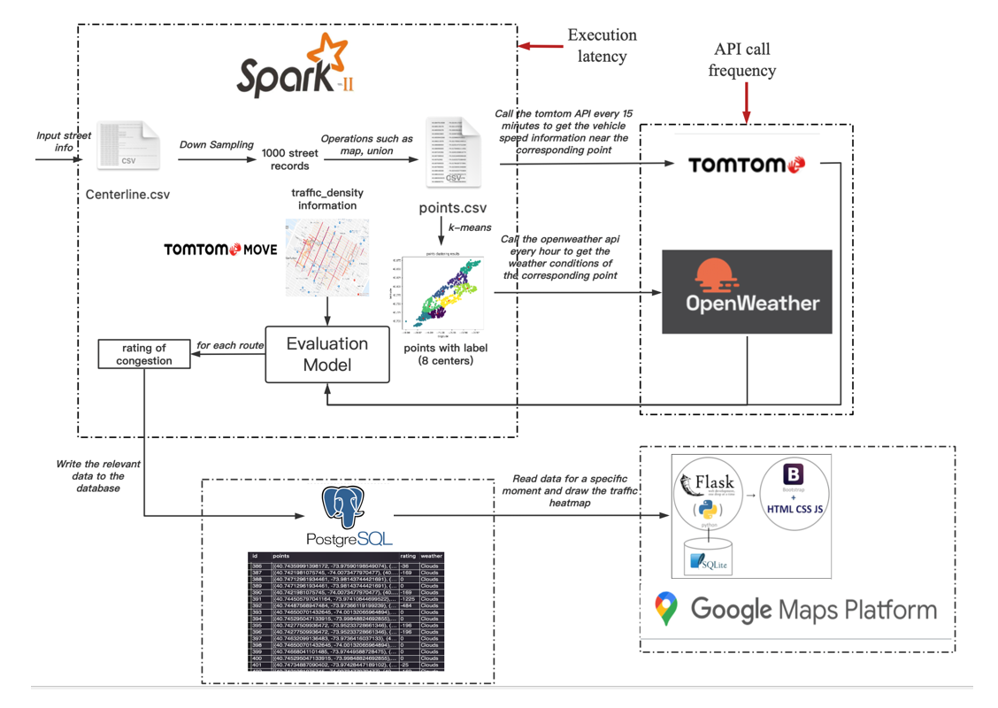
Figure 2.
Streaming processing DAG for input street data
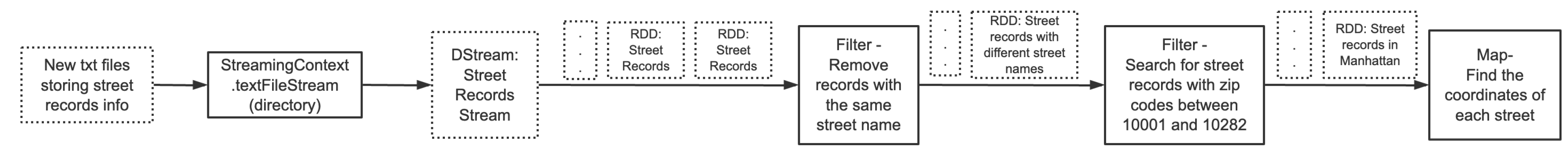
Figure 3.
Streaming processing DAG for Traffic & Weather data
Disclaimer/Publisher’s Note: The statements, opinions and data contained in all publications are solely those of the individual author(s) and contributor(s) and not of MDPI and/or the editor(s). MDPI and/or the editor(s) disclaim responsibility for any injury to people or property resulting from any ideas, methods, instructions or products referred to in the content. |
© 2025 by the authors. Licensee MDPI, Basel, Switzerland. This article is an open access article distributed under the terms and conditions of the Creative Commons Attribution (CC BY) license (http://creativecommons.org/licenses/by/4.0/).
Copyright: This open access article is published under a Creative Commons CC BY 4.0 license, which permit the free download, distribution, and reuse, provided that the author and preprint are cited in any reuse.


