
Submitted:
20 January 2025
Posted:
20 January 2025
You are already at the latest version
Abstract
We developed a web application demo, dynamically monitoring and visualizing the traffic condition in New York City, with a focus on Manhattan. We took advantage of two public API providers: Tomtom and Openweather, for traffic-related streaming data including real-time intersection speed, historical density, and weather details. We proposed a novel congestion model and updated the traffic heatmap every 15 minutes. We implemented our visualization by Google Maps APIs and similar to Google Map layout, we quantified the congestion into three degrees and plotted streets with colors. Our demo achieved similar performance with Google Maps, but with more reasonable and accurate results. Our work can also accept streaming data to achieve high-level concurrency.
Keywords:
Real-time Visualization
; Async Streaming
; Traffic Analysis
1. Introduction
It is challenging to commute in the metropolitan, as road conditions are likely to be ever changing. Moreover, if there is a temporary incident or emergency, for instance, a road closure or traffic accident, the region may be rerouted. There are more than 14,000 roads of all levels, and 13,000 traffic lights in New York City. Roads are densely planned and constructed in grid-like manner, with orthogonal and parallel layout, making route planning with many possibilities and options. Instead of always locating the shortest route, it is better to identify the fastest one under continuously changing traffic.
Based on preliminary investigations, we narrowed our problem into two main challenges: data acquisition and model correction. As we didn’t have access to videos from city surveillance cameras, we sought for alternatives. Among all available tools, [1] developer tool has strong interfaces for accessing both real-time and historical data. Also, we need to count on real-time weather to correct the analysis model. Besides weather impact, there are other external factors, to illustrate, emergent road closure, car crash and special event. We highlighted these areas in the UI to alert drivers. Overall, our contributions are:
- Constructed a more realistic traffic heatmap with real-time speed data, historical density information, and current weather conditions.
- Created a scalable, high-performance backend system capable of processing large volumes of streaming data with minimal latency.
- Created front-end logic for road condition prediction and retrivial.
2. Related Work
2.1. Traffic Flow Modeling
Early work by Lighthill et al. [3] established fundamental diagrams for traffic flow. Their macroscopic model, known as the LWR model, has been a cornerstone in traffic flow theory. More recent studies, such as Treiber et al. [4], Vlahogianni [5] and Lv et al. [6], have incorporated machine learning techniques for improved prediction accuracy. Specifically, they proposed a data-driven approach using neural networks to predict traffic flow patterns. However, these models often lack real-time adaptability to changing conditions, a gap our work aims to address.
2.2. Real-time Data Processing Systems
The advent of big data technologies has enabled more sophisticated traffic analysis. Jagadish et al. [7] provided a comprehensive review of big data challenges and techniques, highlighting the importance of real-time processing in various domains, including traffic management. Building on this foundation, Abbas et al. [8] demonstrated the use of streaming graph analytics for real-time traffic jam detection and congestion reduction. In the context of traffic data, Artikis et al.[9] demonstrated the use of complex event processing for real-time traffic management. They proposed a system that could detect and respond to traffic events in real-time, but their work did not incorporate weather data or historical traffic patterns. Our work builds on these foundations, specifically leveraging Apache Spark for high-throughput stream processing and integrating multiple data sources for a more comprehensive analysis.
2.3. Traffic Visualization Techniques
Visualization plays a crucial role in making traffic data accessible. Chen et al. [12] surveyed various techniques for visualizing urban traffic data, comparing different approaches such as heat maps, flow maps, and 3D visualizations. Zheng et al. [10] further explored the potential of big data for social transportation, highlighting the importance of comprehensive data integration in traffic visualization. Commercial solutions like Google Maps and Waze have popularized the use of color-coded heatmaps for traffic visualization. However, these solutions often rely heavily on user-reported data, which can be inconsistent or biased. Our approach aims to provide a more objective visualization by primarily relying on sensor data and real-time volume information.
3. Methodology
3.1. System Architecture Overview
The system architecture is shown in Figure 1. The whole structure can be divided into three core components: data processing with [11], analysis model with Python, and visualization with Flask and Postgres. We name these components as data processing, congestion algorithm and visualization for simplicity in the following subsections.
We extracted all roads in New York City from [12]. Given a huge amount of data and enormous repetition, the roads were downsampled to an acceptable quantity. Road information is one of the official sources. There are two branches to process these roads. One is served as the request parameters in [1] traffic flow API call, another is used for [2] weather Call. We obtained traffic speed and weather information from the two calls. These will be flowed into the evaluation algorithm. Another input of the algorithm is the traffic density. Given that it is region-based historical data, we can prepare it without explicit geographic coordinates. We roughly separate Manhattan into 24 local regions based on community, and we navigate a specific road density in a hierarchical manner. First we direct the road to the nearest region center, and after that the road will be matched to the nearest segment in the local region with traffic density information. The output of the evaluation model is the traffic congestion score. These scores will be stored in Postgres with current time as table name. The table will be extracted from the Flask and visualized with HTML, CSS, JavaScript developer toolkit on Google Maps Platform.
3.2. Data Processing
Data processing is developed under [11] and Spark Streaming. The static data (road coordinates) was processed by [11] and streaming data was processed by Spark Streaming.
3.2.1. Static Data Processing
In the raw street file provided by [12], there are more than 140,000 road segements. We firstly get rid of repetitive street annotations, with more than 90% of roads were excluded. After that, we restricted the region in Manhattan only by filtering zip code. Ultimately we had 1,000 records as input of the analysis and visualization model. Given less than 10,000 points to call, we could easily store everything in one file. You could either read the points into Spark DataFrame or RDD.
Spark data would be sent through two branches, traffic speed acquisition and real-time weather acquirement. Points could be sent as request parameters in forEach loop. As for traffic speed, there is a huge diversity amongst intersections, as it internally may be impacted by road infrastructure design (number of lanes), and speed limit, and externally is relevant to emergent situations such as road closure and restrictions. Thereby there was no downsampling strategy of traffic speed call. However, unlike continuously diversified traffic conditions, weather is more likely to remain consistent within a small region. We implemented clustering to divide Manhattan into 8 regions with K-Means. We only needed to call the weather at the cluster centroids to represent the regional weather. This approach significantly reduced API call volumes.
3.2.2. Streaming Data Processing
With the extension of the map of interests and time span, we leverage stream processing to deal with high throughputs. With low-volume data, we only downsample and transform the data once, applying the same process consistently in subsequent steps. However, for high-volume streaming data, each batch must be downsampled and transformed as it arrives.
A desirable solution must continuously process and store new data points. Figure 2 illustrates the flow of our streaming data processing in this scenario.
The step of Streaming Context is to create a data stream monitoring for new text files storing street records and load them. The filtering and deduplication strategy is the same as the static processing.
After obtaining the vehicle information corresponding to each street through the [1] Traffic API, we connected the coordinates of each vehicle’s driving route to a coordinate queue, while storing the driving speed and free-flow speed of each vehicle as an RDD. Finally we merged the two into a list. We also continuously updated the cluster centers with new streaming points to get weather details, and broadcast it to all intra-points. Then we transferred processed vehicle trajectories and weather data into the congestion evaluation model for subsequent calculations. Figure 3 shows the detailed processing flow.
3.2.3. Streaming Strategy
Since we are developing a real-time traffic heatmap, low processing latency is crucial. We found that the most time-comsuming step lies on the API calls, especially the [1] traffic flow APIs. For each API call, it consists of overhead for session establishment and request/response for GET/POST request. The first optimization we could implement is to reduce overhead cost by keeping live a session all the time. This will prevent establishing a session for every API call.
We found that all API calls are relevant to the requested points and are independent with each other. We regarded the API calls as stateless operations and the further improvement was to have asynchronized API calls. Figure 4 shows the time-series execution logic. Two third-party packages achieve this: asyncio and aiohttp. The former one is used to set up co-routine and achieve high-level of asynchronism, and the latter is served as a middleware in the web-server. There are two keywords of triggering asynchronous call: async and await, where first one is the signal of activating a co-routine and the second one is a signal of interruption of executing the asynchronous program.
Regarding our backend module as a multi-task system, we could optimize the streaming data processing with FAIR scheduler. The resource manager is a variant of YARN scheduling by assigning weights to tasks. If two significantly different and stateless tasks with different resources and were executed sequentially and difficult job started first, it is likely that the hard job would take up all the computing resources, and the easy job would be executed only after the difficult job was completed. FAIR scheduler will assign unique proprity to each task, and allocate resources to all jobs to avoid unnecessary idle status. In Apache Spark, each job is called a pool, separating resources of different clients. We used weight to set up job priority and minShare to avoid the scheduler being downgraded into FIFO manner.
3.3. Congestion Algorithm
Traditional traffic flow theory empirically validates traffic congestion is inversely proportional to traffic flow, presented in notation 1, where f is traffic flow, D is density, V is velocity, and is a calibration coefficient determined from historical data.
Through extensive analysis of real-world traffic patterns in Manhattan, we discovered that this traditional model, while theoretically sound, fails to capture several critical aspects of urban traffic dynamics. Most notably, the linear relationship between density and congestion does not accurately reflect real-world scenarios. For instance, high traffic density on expressways often represents efficient vehicle flow rather than congestion, while low density during off-peak hours may not necessarily indicate smooth traffic conditions. Figure 5 shows the basic curve of traffic flow with respect to traffic density.
To address these limitations, we correct our evaluation model by having a small punishment with high and low traffic density. We also added weather impact to free-flow speed as expected speed, and evaluated the speed deviation with L2 distance. Weather coefficients are emperical, summarized from [13]. Also, we found there was a scaling difference between speed deviation and density punishment, and following the idea of the original congestion calculation having both factors equal contributions, we refactored density punishment from D to . The ultimate evaluation is shown in notation 2, where W is weather coefficient, fs is free-flow speed and cs represents current speed.
3.4. Visualization
The visualization was built on [14]. We took advantage of Maps JavaScripts API and roads API. Our scorings include segment coordinates, weather and congestion scores. We quantized the scores with two thresholds: -100 and -500, and indicated three degrees: no congestion (green), slight congestion (orange) and heavy congestion (red). The visualization also includes alert of historical car crash incidents as black dots. Except real-time traffic heatmap visualization, we supported playback of past 24-hour traffic condition change and navigation back to the latest traffic condition given a specific weather. We now support rainy, snowy, foggy and tornado playbacks. The screenshot is shown in Figure 6.
There are two major difficulties during implementation, first is the visualized data needing to be post-processed before being read by JavaScript for data format and precision adjustment. We used Flask to build a middleware between the Postgres cursor and JavaScript. Frontend will send a POST or GET request through Flask, the cursor will fetch corresponding data from Postgres. Second is that the route drawing response is slow and inefficient with large quantity of data. To avoid an awkward situation where the map was not filled, we found that there is no need to clear the map every time before the traffic congestion was updated. Instead, we can keep the old traffic condition visualization and draw lines on top of the old lines. Once the update is completed, we can clear the old visualizations.
4. Results
4.1. Qualitative Results
Our proposal leverages real-time data source and achieves real-time traffic condition every 15 minutes, and the traffic condition can be upscaled to a larger area without API traffic limit. We are also able to replay history traffic condition and weather information for continual learning of the forcasting model.
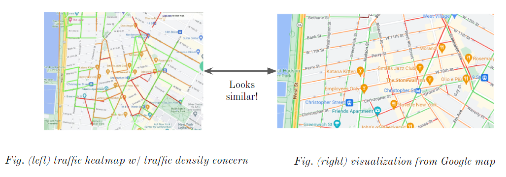
While it is hard to systematically measure the accuracy the traffic condition, we asked a few New York resident volunteers to monitor their neighborhood road conditions, and compared their observation with both Google Maps and our demo. Our demo performs better on side and single-directional roads, where traffic volume is generally low and congestion is less likely to occur.
A typical example was on the west side of Manhattan downtown, a dense area with tens of intersections at 8 pm, May 5th. We compared our result with Google Map. In Figure 7, we found that the visualizations, while are similar in coloring, ours suggesting lighter traffic on side Roads and heavier traffic on major avenues.
4.2. Quantitative Results
Benefited by asynchronized API calls, our implementation can accelerate streaming data fetch from 3.66 seconds per 50 calls to 0.29 seconds per 50 calls. The overall processing time for a 15-minute interval is shortened to 4 minutes with spark RDD vectorization and FAIR scheduler.
5. Review and Future Work
We developed a web application upon Google Maps Platform. As we developed our demo with limited time, there is still room for improvement. Based on the feedback from the presentation, we concentrate our future work to three issues:
We may deploy our application to cloud servers to support multi-user access. We can upload our program to Google Cloud Platform. We can store our data in BigQuery and set our scheduler via Airflow, with program triggered every 15 minutes.
We may expand our heatmap to route recommendations. We can leverage Google Maps Direction API to present candidate routes from one place to another and combine our heatmap to determine the fastest route. Besides, we can leverage the current speed from [1] API to calculate expected commuting time.
We may leverage window function to smooth our playback. We can set up a time interval window and slide the window to exclude older data and accept newer data and the playback can be smoothed from GIFs to videos.
References
- Tomtom. tomtom. [EB/OL], 2022. https://developer.tomtom.com/ Accessed , 2022. 8 May.
- openweather. openweather. [EB/OL], 2022. https://openweathermap.org/api Accessed , 2022. 8 May.
- Lighthill, M.J.; Whitham, G.B. On kinematic waves II. A theory of traffic flow on long crowded roads. Proceedings of the royal society of london. series a. mathematical and physical sciences 1955, 229, 317–345. [Google Scholar]
- Treiber, M.; Kesting, A. Traffic flow dynamics traffic flow dynamics. In Data, Models and Simulation; Springer-Verlag Berlin Heidelberg, 2013; pp. 983–1000.
- Vlahogianni, E.I.; Karlaftis, M.G.; Golias, J.C. Short-term traffic forecasting: Where we are and where we’re going. Transportation Research Part C: Emerging Technologies 2014, 43, 3–19. [Google Scholar] [CrossRef]
- Lv, Y.; Duan, Y.; Kang, W.; Li, Z.; Wang, F.Y. Traffic flow prediction with big data: A deep learning approach. Ieee transactions on intelligent transportation systems 2014, 16, 865–873. [Google Scholar] [CrossRef]
- Jagadish, H.V.; Gehrke, J.; Labrinidis, A.; Papakonstantinou, Y.; Patel, J.M.; Ramakrishnan, R.; Shahabi, C. Big data and its technical challenges. Communications of the ACM 2014, 57, 86–94. [Google Scholar] [CrossRef]
- Abbas, Z.; Sottovia, P.; Hassan, M.A.H.; Foroni, D.; Bortoli, S. Real-time traffic jam detection and congestion reduction using streaming graph analytics. In Proceedings of the 2020 IEEE International Conference on Big Data (Big Data). IEEE; 2020; pp. 3109–3118. [Google Scholar]
- Artikis, A.; Weidlich, M.; Gal, A.; Kalogeraki, V.; Gunopulos, D. Self-adaptive event recognition for intelligent transport management. In Proceedings of the 2013 IEEE International Conference on Big Data. IEEE; 2013; pp. 319–325. [Google Scholar]
- Zheng, X.; Chen, W.; Wang, P.; Shen, D.; Chen, S.; Wang, X.; Zhang, Q.; Yang, L. Big data for social transportation. IEEE transactions on intelligent transportation systems 2015, 17, 620–630. [Google Scholar] [CrossRef]
- Spark, A. Spark. [EB/OL], 2022. https://spark.apache.org/docs/latest/index.html Accessed , 2022. 8 May.
- OpenData, N. nyc opendata. [EB/OL], 2022. https://opendata.cityofnewyork.us/ Accessed , 2022. 8 May.
- Hani, S. Mahmassani, Jing Dong, J.K.; Chen, R.B. Incorporating Weather Impacts in Traffic Estimation and Prediction Systems. [EB/OL], 2009. https://rosap.ntl.bts.gov/view/dot/3990.
- maps platform. maps platform. [EB/OL], 2022. https://developers.google.com/maps/documentation Accessed , 2022. 8 May.
Figure 1.
System Architecture
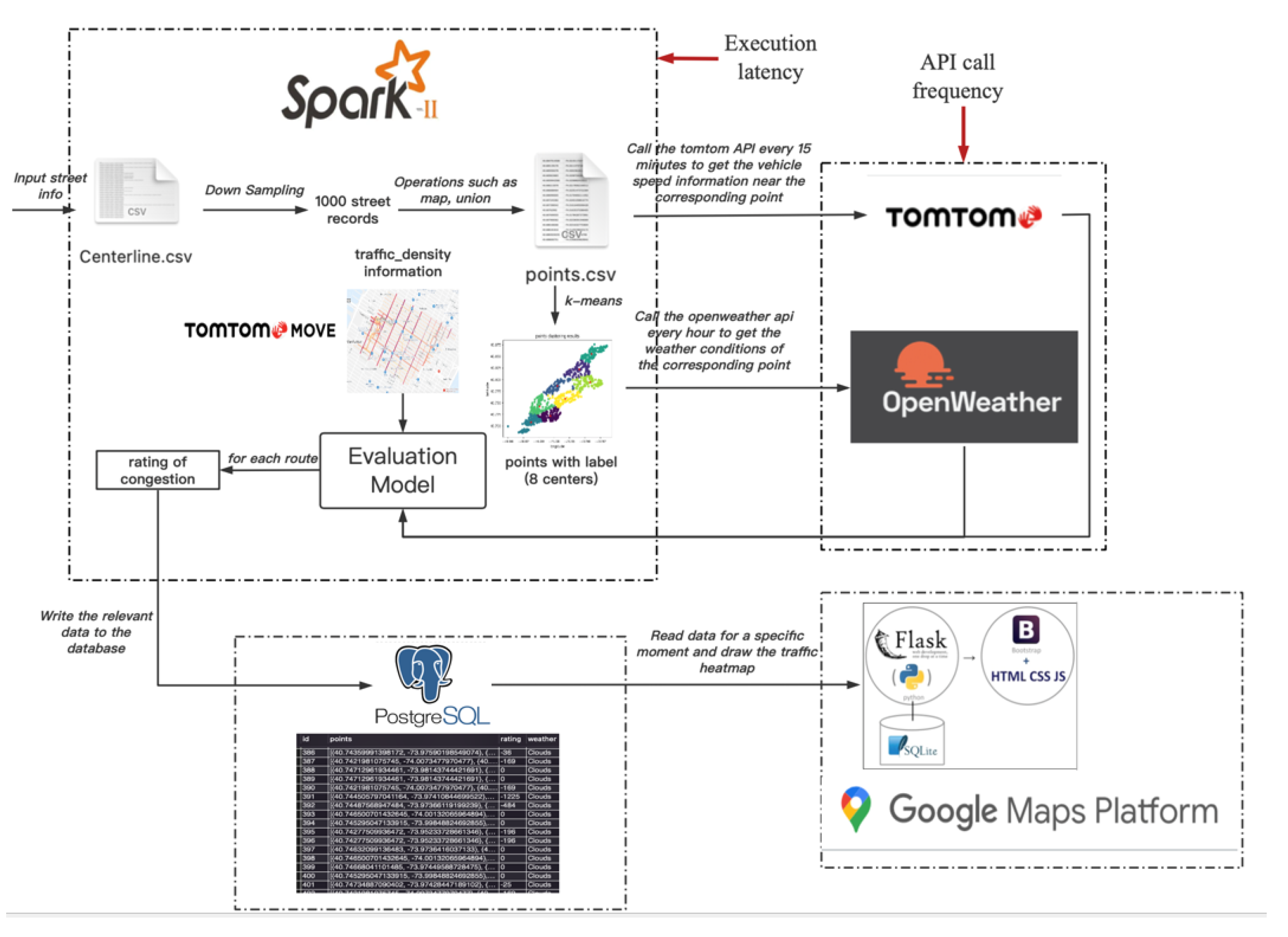
Figure 2.
Streaming processing DAG for input street data
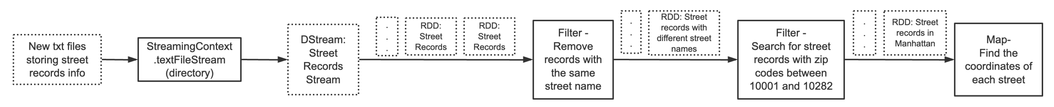
Figure 3.
Streaming processing DAG for Traffic & Weather data
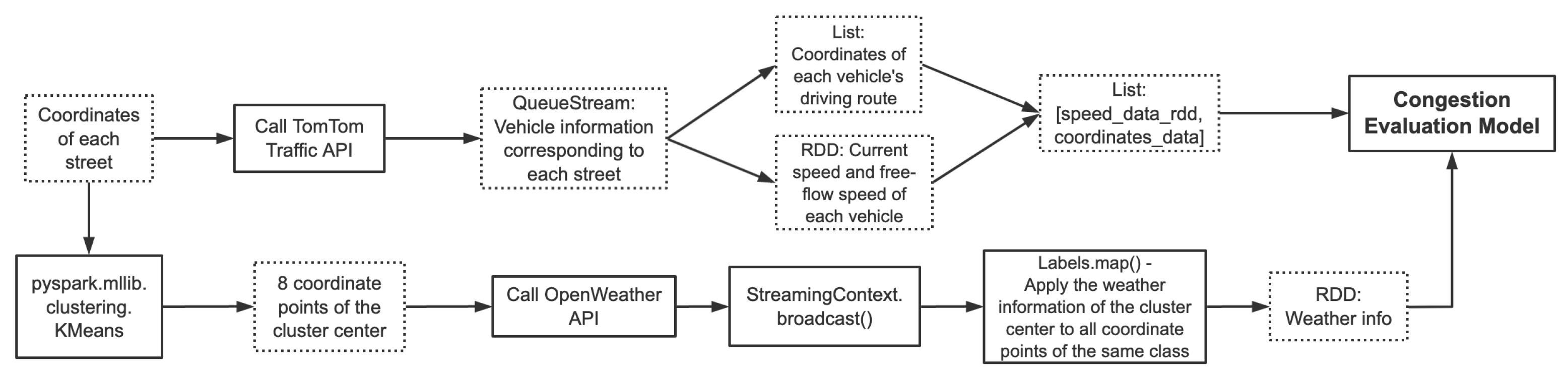
Figure 4.
async API Call
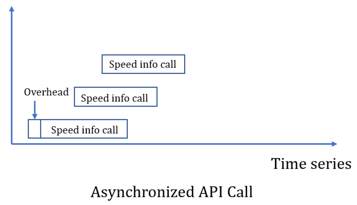
Figure 5.
Fundamental traffic flow curve
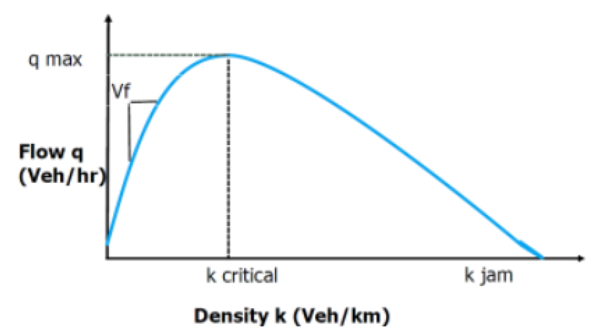
Figure 6.
Visualization screenshot
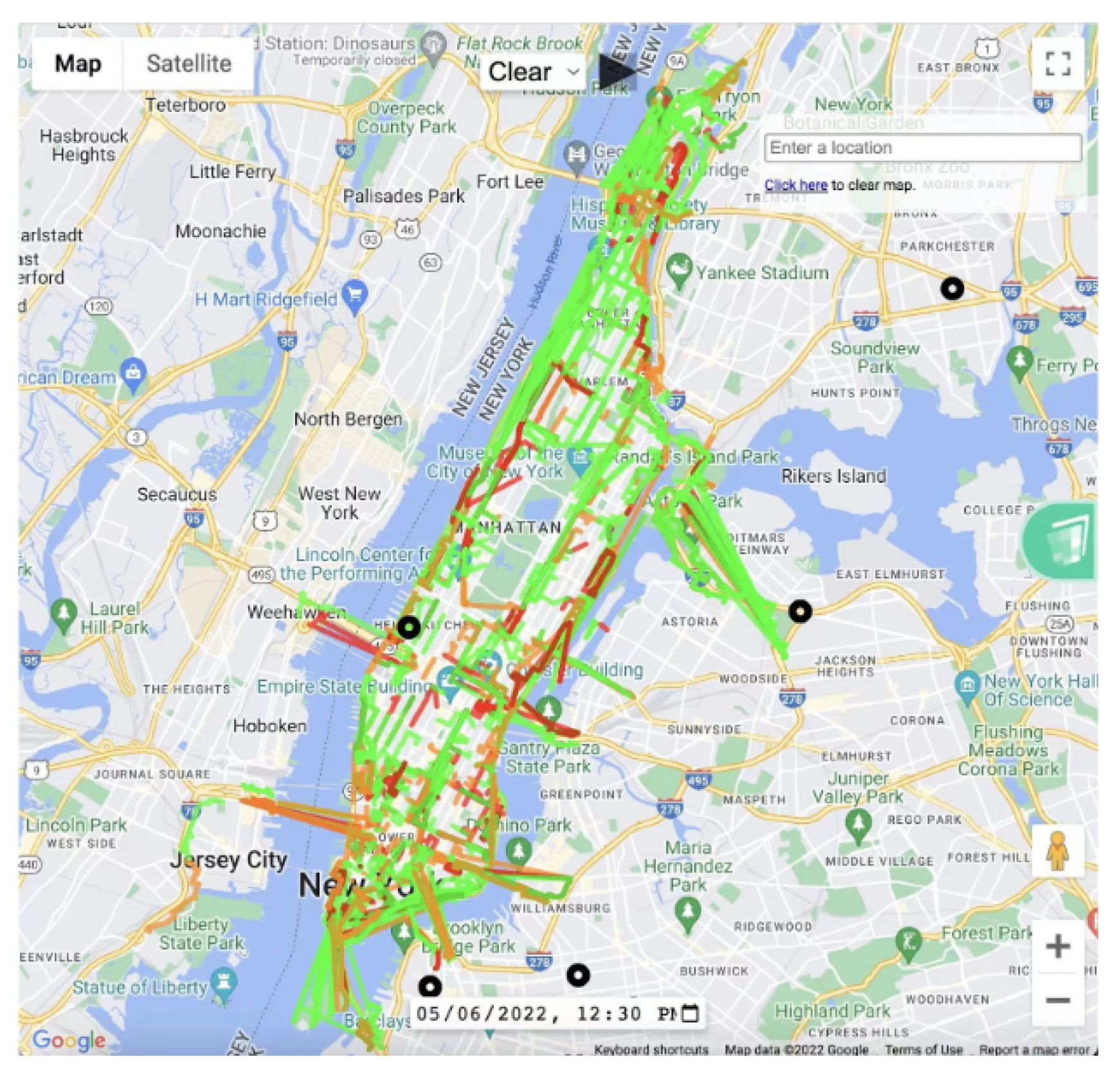
Figure 7.
Evaluation comparison
Disclaimer/Publisher’s Note: The statements, opinions and data contained in all publications are solely those of the individual author(s) and contributor(s) and not of MDPI and/or the editor(s). MDPI and/or the editor(s) disclaim responsibility for any injury to people or property resulting from any ideas, methods, instructions or products referred to in the content. |
© 2025 by the authors. Licensee MDPI, Basel, Switzerland. This article is an open access article distributed under the terms and conditions of the Creative Commons Attribution (CC BY) license (http://creativecommons.org/licenses/by/4.0/).
Copyright: This open access article is published under a Creative Commons CC BY 4.0 license, which permit the free download, distribution, and reuse, provided that the author and preprint are cited in any reuse.


