
Submitted:
09 January 2025
Posted:
13 January 2025
You are already at the latest version
Abstract
In this paper, we propose a novel model that is based on a hybrid paradigm composed of graph convolution network and Integer Programming solver. The model utilizes the potential of graph neural networks that have the ability to capture complex relationships and preferences among nodes. As the graph neural network forms node embeddings that are fed as input to the next layer of the model, the introduced MILP solver works to solve the team formation problem. Eventually, the experimental work shows that the outcome of the model is balanced teams.
Keywords:
Team Formation Problem
; graph neural network
; graph convolution network
; 8 Mixed Integer Linear Programming
; node embeddings
1. Introduction
Effective team building is crucial for successful projects. Research indicates that well-composed teams increase productivity, motivation, job satisfaction, and overall project outcomes [1]. This complex issue is relevant across diverse fields like education, healthcare, sports, and software development, wherever group work is necessary. However, teams often perform poorly despite individual efforts due to issues such as poor communication, conflict, ineffective knowledge sharing, ambiguous goals, and unclear roles. The Team Formation Problem (TFP) is a challenging optimization problem focused on creating effective teams while considering numerous factors. Defining "effective" varies by context; some projects prioritize maximizing combined skills, while others focus on minimizing conflict or enhancing adaptability. Team composition can also vary depending on the task, with some favoring heterogeneous teams based on demographics, personality, or past performance, and others preferring homogeneous groups. The TFP’s complexity increases with the pool of potential members and the number of constraints, making it computationally challenging (NP-hard). Various solutions exist, from simple brute-force methods to complex metaheuristics like Particle Swarm Optimization, Genetic Algorithms, and others. This research aims to categorize the most common optimization techniques used to solve the TFP based on their approach (exact, approximation, or hybrid) and application domain (e.g., education, sports, healthcare). Despite extensive research, a clear overview of existing literature is lacking due to varying results. This review synthesizes and evaluates the literature to highlight the most effective and frequently used techniques. These classifications will help professionals select appropriate algorithms for their projects based on the specific application domain.
In addition and under various names, such as coalition structures (CS), one can find out that the topic has been extensively studied in intelligent agents (IA) [2,3,4]. Research on IA aims to maximize utility for both individual agents and teams (either the total team’s utility or the average utility of each team member), specifically the likelihood of agents leaving their current group to join another. This problem, whether referred to as Team Formation (TFP) or Coalition Structure (CS) formation, remains NP-hard.
However, as a classification of the majority of algorithms proposed to solve the TFP, we reach the conclusion that approximate algorithms constitute the largest group of techniques employed to address the Team Formation Problem (TFP) due to their reduced computational demands. These algorithms prioritize finding a satisfactory solution rather than the absolute best. Typically non-deterministic and operating in polynomial time, they are favored when dealing with a large number of potential solutions. This category is broadly divided into heuristics and metaheuristics (MH). Metaheuristics are further classified as single-solution MH and population-based MH. Single-solution algorithms iteratively refine a single solution and target to converge on a local optimum. These are suitable for single-team formation scenarios. In contrast, population-based algorithms concurrently modify multiple solutions. As their convergence rate is generally slower than that of single-solution algorithms, they are better suited for problems involving the formation of multiple teams. Population-based techniques can be further subdivided into evolutionary algorithms (including the widely used Genetic Algorithm) and swarm-based or animal-inspired algorithms, such as Ant Colony Optimization (ACO), Bee Colony Optimization (BCO), and Crow Search Algorithm (CSA). Finally, hybrid algorithms combine distinct approaches, such as exact methods and MHs, or two different MH techniques.
This work is different from the work proposed by Farasat and Nikolaev [5] in that Farasat and Nikolaev aim is to capture the social structure in terms of forming different graph representations, namely network structure measures (NSMs). Then, they the feed the formed NSMs to the proposed mathematical model to form teams. From our point of view, the goal of capturing social structure among other features, such as preferences and complex interactions, could be easily addressed using GNNs.
Thus, the contribution of this work is three-fold. First, we introduce the concept of balanced team formation and employ GCNs to form node embeddings and capture the important features of the participating peers. Second, we introduce a mathematical model that appears in the novel MILP solver to help form balanced teams. Third, we reinforce this with experimental results to validate the proposed model.
2. Related Work
The work of Bhowmik et al. [6] propose a simulated annealing algorithm (SA) to the problem of team formation. They deal with the problem as a submodular function optimization (SFO). In general, SFO is an NP-hard problem. Bhowmik et al. formulate the problem as a graph network, , where V denotes the set of experts, E denotes the set of edges between the experts and W denotes the communication cost between the experts. Then, they introduce the principle of submodularity (SM) in three major areas, e.g., skill coverage. In addition, they argue that the SM is satisfied for skill coverage if for every project P that requires a set of skills, the formed team T has coverage for all required skills in the project. The downside of the proposed work is that SA in general suffers from slow convergence and sensitivity to parameter choice. In addition, the weighted edges model the communication costs among the experts and overlook the integration of roles or preferences.
However, the wok proposed by Farasat and Nikolaev [5] proposes a mathematical model for the team formation problem (TFP). In addition, they extend the TFP by embedding a social structure (SS) which yields the problem (TFP-SS). Also, they express the TFP-SS as an undirected graph with a disregard to edges’ weights, . They propose an Integer Programming (IP) algorithm to solve the proposed TFP-SS.
Chalkiadakis and Boutilier [7] address the TFP in different context. They propose a model to solve coalition formation problem in multi-agent applications using a Bayesian reinforcement learning-based model. Their proposed model exhibits a tradeoff between exploration (of new partners for potential coalition formation) and exploitation of the existing coalition.
In addition, Yeh [8] proposes a dynamic programming algorithm to address the complete set partitioning problem. However, the algorithms that are proposed in [8] can be adapted to solve the Coalition Structure Generation (CSG) problem.
Sen and Dutta [9] study the formation of coalitions in IA using order-based genetic algorithm (OBGA).The authors introduce a new algorithm called the "Optimal Bi-level Genetic Algorithm" (OBGA). This algorithm uses a genetic algorithm approach, which is a type of search algorithm inspired by natural selection. Here’s how it works: Bi-level Structure: The OBGA has two levels. The outer level: This level searches through the space of possible coalition structures. It represents each coalition structure as a "chromosome" (a string of information).Then, the inner level: For each coalition structure generated by the outer level, the inner level calculates the value or utility of that structure. This is often done by solving a subproblem related to how the agents within each coalition will cooperate.
Sharaf and El-Ghazawi [10] propose a coalition fromation model to serve in the domain of fog computing. They propose a model that is based on Markov Chain Monte Carlo (MCMC). The model can incorporate a set of nodes’ preferences that guide the formations of coalitions.
The work by Zhang and Hu [11] follows the same goal of coalition formation stated by Sharaf and El-Ghazawi [10] to utilize the coalition formation to serve computational aspects at the edge. Zhang and Hu propose a model that is based on M-ary discrete particle swarm optimization (MDPSO).
To sum up, generating coalition structures and TFP both are computationally complex (NP-hard) problems [2,12,13], making the search for optimal solutions impractical due to their exponential time requirements. Consequently, much research has focused on finding good, but not necessarily perfect, solutions. One such attempt is the work of Chalkiadakis et al. [14] where they propose a greedy algorithm for the set-covering problem. However, the proposed model solves a variant of the problem, namely the ovelapping coalition formation (OCF). Therefore, Chalkiadakis’ algorithm is not suitable to our problem because our approach requires teams to be disjoint (i.e., no player can belong to multiple teams).
3. Graphical Convolutional Network
Graph Neural Networks (GNNs) have emerged as a powerful tool for analyzing data represented as graphs. The foundational work on GNNs was presented by Gori et al. in 2005 [15]. Subsequent research by Scarselli et al. [16] and Gllicchio et al. [17] further developed and clarified the GNN concept. These early GNN models relied on an iterative message-passing process, where information is exchanged between neighboring nodes until a stable state is reached. However, this iterative approach proved to be computationally expensive. A significant breakthrough came with the introduction of Graph Convolutional Networks (GCNs) by Kipf and Welling in 2016 [18]. GCNs offer a more efficient way to aggregate information from neighboring nodes, drawing an analogy to Convolutional Neural Networks (CNNs) used for image processing. Just as CNNs use kernels to aggregate information from neighboring pixels, GCNs aggregate information from neighboring nodes as shown in Figure 1. Bronstein et al. [19] highlighted the importance of adapting neural network architectures to non-Euclidean data structures, where graph representations are particularly suitable, citing examples in social networks, molecular chemistry, and gene expression. While GNNs have demonstrated great potential in tasks like classification and link prediction, graph clustering remains a challenging task for existing approaches as they often struggle to outperform even basic algorithms like K-means, see Tsitsulin [20].
4. Proposed GCN-MILP Model
In balanced coalitions and teams, we aim at having groups of balanced potentials and equal at best. While grouping candidates by features might not yield homogeneous teams, we argue that GNN can provide more accurate approach for the following reasons:
- Each candidate is represented as a node with features like skill, experience, position, power, etc.
- GNN can learn rich representations for each candidate by considering their relationships(edges) with other candidates along with their individual features(attributes).
We formulate the problem as a clustering problem with constraints. Once the GNN model has learned the node embeddings, clustering algorithms can be applied to group candidates into teams/coalitions. However, we constrain the formation by ensuring that the embeddings among teams/coalitions are as similar as possible to provide for balanced and homogeneity as possible.
4.1. GNN Architecture for Balanced Teams Formation
In this work, we consider the graph-convolutional network (GCN) as the most suitable GNN architecture due to its ability to capture the underlying structure of the candidates in the network.
A GCN builds node embeddings by combining information from neighboring nodes. This is shown in Equation 1.
where:
- : Adjacency matrix with self-loops.
- : Degree matrix of .
- : Node embeddings at layer l ().
- : Learnable weight matrix for layer l.
- : Activation function (e.g., ReLU).
Next, we explore the Components of a GCN for TFP:
-
Input:
- Each candidate is represented as a node with a feature vector containing attributes specific to the case; see Experimental section.
- The relationships among candidates are defined as an adjacency matrix.
-
First layer:
- GCNConv(input_dim, hidden_dim): This layer propagates information along edges, aggregating information from neighboring nodes.
- This helps in capturing higher-order relationships between candidates
- F.relu(x): It applies a ReLU activation function to introduce non-linearity.
-
Second layer:
- GCNConv(hidden_dim, output_dim): this layer, node embedding, is generated for each candidate in which the importance of each candidate within the network is captured.
- F.relu(x): Another ReLU activation is applied.
- Output: The final output is the node embeddings.
Figure 2 shows the proposed model.
After obtaining the node embeddings, we have to work around the possible clustering of imbalanced teams. The approach we apply to achieve this goal relies on constraint-based clustering in which we employ Integer Programming (IP). Therefore, we formulate the last phase of team formation as an IP problem in which we can define several constraints as team size, minimum skill level, etc. In addition, constraint propagation and backtracking is necessary to find feasible solutions that satisfy the constraints.
4.2. MILP Model
The main objective function of this model is to minimize the difference in cumulative potential levels between teams, DCPLT for short. Then, we introduce the mathematical formulation of the proposed MILP model. First, we define the decision variables.
Decision Variables:
- : Binary variable, 1 if player i is assigned to team j, 0 otherwise.
Parameters:
- n: Number of players.
- m: Number of teams.
- p: Number of players per team.
- : skill level of the player i.
- Weighting factor for relative importance.
Objective Function:
Minimize:
Constraints:
- Player assignment:
- Team size:
- Binary restriction:
Where the is the required number of teams, is the total number of candidates, denotes the computed candidate embeddings and represents a two-dimensional matrix of assignment of size (, ). In the assignment matrix, a cell has a value one if the candidate is a member of the team or zero if it is not a member. The first constraint represents a validity check that must be satisfied by having each candidate as a member of one team at most. While the second constraint verifies that each team has p members at most.
We use PuLP [21] which includes a default solver algorithm, CBC (COIN-OR Branch-and-Cut) [22]. PuLP is an open-source solver capable of treating a broad range of LP problems. In addition, PuLP allows the usage of APIs to enable the usage of other solvers (GUROBI, GLPK, CPLEX, etc.). Figure 3 shows the model pipeline and the collaboration between GCN and the MILP solver.
5. Proposed Balanced Teams Formation Algorithm
Generally, we consider TFP as a variation of the Set Partition Problem (SPP), see [23] for more details on SPP. In addition, SPP is a variation of the Set Covering Problem (SCP). Also, set covering problem is considered since all the constraints are 0-1 integer problems see [24] for more details on constraint programming. We occasionally use ILP (Interger Linear Programming) to solve SPP, see [25] for more details.
The proposed Algorithm 1 addresses the formulated problem and provides a novel model and takes into account additional constraints. The goal is to create a partition that matches the features of the group members (players). In addition, there are roles that are represented in players’ features and preferences that must be adhered to in order to form balanced teams.
| Algorithm 1:GCN and MILP Algorithm |
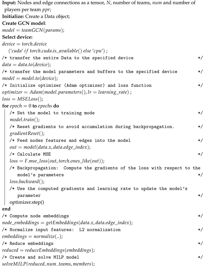 |
5.1. Experimental Work
For experimental purposes, we have designed a network of fifteen players. Each player has a set of skills represented in vector format. The skills are [`Attack’, `Defense’, `Speed’, `Stamina’, `Teamwork’]. Then, we compute a one-dimensional skill based on weights (preferences) that sum to one, e.g. [0.2, 0.3, 0.1, 0.2, 0.2] as shown in Equation 8. In this setting, we prefer the defense skill more than the others.
To sum up the proposed pipeline from end to end, the workflow fits together as follows:
-
Input: Graph is represented in adjacency matrix A and a feature matrix X.
- A: matrix, where if there is an edge between node i and node j, otherwise 0.
- X: matrix is the number of features per node.
- GCN: Generate node embeddings.
- Optimizer: Use embeddings to form balanced teams.
- Output: Team assignments and skill balance metrics.
Therefore, the pipeline outcome is a function of every stage performance. Thus, a well-trained GCN is mandatory to ensure the best encoding of the nodes to facilitate the work of the second stage, i.e., the MILP optimizer. In the proposed model, the GCN provides the node embeddings that encapsulate both node features and the graph structure as input to the oprimizer. However, the quality of the embedding is key in several factors: GCN architecture (e.g., number of layers, hidden dimensions), training process (e.g., loss function, optimization algorithm), and input graph structure and node’s features.
5.2. Experimental Results and Analysis
One of the measures that we employ to gauge the dynamic of teams and the diversity of skills that could be required for certain applications is the Gini coefficient, ratio, or index; see Equation 6. Originally, Gini ratio is used in economics as an indicator of income equality. Practical results indicate that the lower the Gini ratio, the better the equality. Since we have two factors that are addressed in this work, i.e., teams homogeneity and diversity, we can interpret the Gini ratio as follows:
- A low Gini ratio indicates that all members of the team have the same skills. This could be in favor of homogeneity.
- A high Gini ratio indicates that all team members have different skills, i.e., due to the need for different roles within the team. This could be in favor of diversity.
However, the Gini ratio alone may not provide enough insight into team dynamics. For this purpose, we add other complementary metrics, such as variance of skills within each team, average skill level per team, and the standard deviation of skills. In addition, some auxiliary plots can help us perceive the skill distribution across multiple dimensions for each formed team. However, we encountered some limitations in the experimental work due to the adoption of norm-based reduction. while reducing the embedding vectors to 1D can facilitate the work of the MILP model because it effectively captures the magnitude of the feature vectors and simplifies the computational complexity, such reduction leads to loss of directional information as we only retain the magnitude. To illustrate the idea, we consider three-player features represented in the following listing.
- import numpy.linalg as nl
- ’’’
- Example embeddings:
- (3 players, 5 skill dimensions)
- [Defense, Attack, Stamina, Teamwork, and
- Speed]
- ’’’
- player_features = np.array([
- [0.8, 0.7, 0.9, 0.85, 0.7],
- [0.6, 0.9, 0.8, 0.75, 0.7],
- [0.7, 0.65, 0.85, 0.8, 0.75]
- ])
- # Compute the L2 Norm for each player
- norms = nl.norm(player_features, axis=1)
- # The L2 Norm will look like:
- # Expected output
- Player norms: [1.77552809
- 1.69189243
- 1.68448805]
The above feature vectors are replaced by feature norms (e.g., L2 norm) as a scalar as shown in Equation 7.
where d denotes the feature vector dimension, i denotes player i. The resulting player norms shown in the listing clearly reflect the fact that the variations/strengths across the five dimensions have dissolved when we opted for the magnitude only. However, simplifying the MILP is possible while retaining some vector information. This can be achieved by dimensionality reduction techniques, for example, Principal Component Analysis (PCA), or autoencoders, or weighted norms, as shown in Equation 8.
5.3. Experimental Analysis
The first experiment that we present has an optimal solution. The first experiment has the following settings:
- # Skills
- skills = [’Attack’, ’Defense’, ’Teamwork’]
- num_players = 9
- num_skills = 3
- num_teams = 3
- skill_vectors =[
- [0.7,0.4, 0.80], [0.70,0.40, 0.80],
- [0.70,0.40, 0.80],[0.80,0.60,0.40],
- [0.80,0.60,0.40], [0.80,0.60,0.40],
- [0.50,0.90,0.40], [0.50,0.90,0.40],
- [0.50,0.90,0.40]]
The results shown in Figure 4 confirm that the teams formed are balanced. Moreover, we calculate the Gini Coef. and tabulate the results in Table 1. The Gini ratios demonstrate homogeneity and equality among teams.
Next, we present a second experiment with the following settings: a pool of twenty players; each has three skills. The objective is to form four teams each of size five.
The results of the experiment are shown in Table 2.
Interpretation of metrics:
- Mean Skill Distance (MSD): Lower values signify fair skill distribution.
- Within-Team Variance (WTV): Lower values signify cohesive teams.
- Skill Balance (SB): Lower values signify balanced teams.
First, the MSD score of 0.6222 indicates, on average, that individuals are close to the average skill level of their respective teams. This suggests that the teams formed are homogeneous in terms of individual skill levels. Second, the WTV score of 1.695 confirms that the teams are fairly homogeneous. Finally, the SB score of 0.1052 is a favorable low value that indicates that the average skill levels among all teams are very similar. Thus, we can deduce that the proposed model successfully generates teams with a balanced distribution of skills.
6. Discussion
Using GNNs to better represent relationships and preferences in team formation has the potential to produce a solution with the best needed quality. The merits introduced by GNN models exceed the basic skill-based comparisons. Our approach aims to form balanced teams that witness a minimization of the variance in skill levels between the teams.
7. Conclusion and future work
Graph neural networks have shown flexibility in understanding relationships between entities, incorporating preferences, and learning complex interactions between domain-specific nodes. Using graph convolution networks (GCNs) to address the team formation problem offers the advantage of flexibility and adaptability in terms of its ability to reflect network dynamics and relationships. In this work, we propose a hybrid model of GCN and MILP to solve the team formation problem. Based on experimental work, the proposed model is capable of obtaining the optimal solution if it exists. A possible shift to heuristic, metaheuristic or greedy approaches can provide a near optimal solution in a reasonable time even if they are not guaranteed to provide the optimal solution. Future work may see the employment of graph attention networks (GATs) as GATs use an attention mechanism that provides the ability to provide better feature learning and dynamic weighting. Additionally, GATs have better interoperability, flexibility (diverse relationships between nodes and inductive bias), and performance.
References
- Kumar, S.; Deshmukh, V.; Adhish, V.S. Building and leading teams. Indian journal of Community medicine 2014, 39, 208–213. [Google Scholar] [CrossRef]
- Dang, V.D.; Dash, R.K.; Rogers, A.; Jennings, N.R. Overlapping coalition formation for efficient data fusion in multi-sensor networks. In Proceedings of the AAAI, Vol. 6; 2006; pp. 635–640. [Google Scholar]
- Su, Z.; Zhang, G.; Yue, F.; He, J.; Li, M.; Li, B.; Yao, X. Finding the largest successful coalition under the strict goal preferences of agents. ACM Transactions on Autonomous and Adaptive Systems (TAAS) 2020, 14, 1–33. [Google Scholar] [CrossRef]
- Rahwan, T.; Ramchurn, S.D.; Dang, V.D.; Giovannucci, A.; Jennings, N.R. Anytime optimal coalition structure generation. In Proceedings of the AAAI, Vol. 7; 2007; pp. 1184–1190. [Google Scholar]
- Farasat, A.; Nikolaev, A.G. Social structure optimization in team formation. Computers & Operations Research 2016, 74, 127–142. [Google Scholar] [CrossRef]
- Bhowmik, A.; Borkar, V.; Garg, D.; Pallan, M. , Submodularity in Team Formation Problem. In Proceedings of the 2014 SIAM International Conference on Data Mining (SDM); pp. 893–901. [CrossRef]
- Chalkiadakis, G.; Boutilier, C. Sequentially optimal repeated coalition formation under uncertainty. Autonomous Agents and Multi-Agent Systems 2012, 24, 441–484. [Google Scholar] [CrossRef]
- Yun Yeh, D. A dynamic programming approach to the complete set partitioning problem. BIT Numerical Mathematics 1986, 26, 467–474. [Google Scholar] [CrossRef]
- Sen, S.; Dutta, P.S. Searching for optimal coalition structures. In Proceedings of the Proceedings Fourth International Conference on MultiAgent Systems. IEEE; 2000; pp. 287–292. [Google Scholar]
- Sharaf, M.; El-Ghazawi, T. Preference-based and homogeneous coalition formation in fog computing. In Proceedings of the 2019 IEEE Conference on Standards for Communications and Networking (CSCN). IEEE; 2019; pp. 1–6. [Google Scholar]
- Zhang, K.; Hu, Y.; Tian, F.; Li, C. A Coalition-Structure’s Generation Method for Solving Cooperative Computing Problems in Edge Computing Environments. Information Sciences 2020, 536. [Google Scholar] [CrossRef]
- Sandholm, T.; Larson, K.; Andersson, M.; Shehory, O.; Tohmé, F. Coalition structure generation with worst case guarantees. Artificial intelligence 1999, 111, 209–238. [Google Scholar] [CrossRef]
- Shehory, O.; Kraus, S. Methods for task allocation via agent coalition formation. Artificial intelligence 1998, 101, 165–200. [Google Scholar] [CrossRef]
- Chalkiadakis, G.; Elkind, E.; Markakis, E.; Polukarov, M.; Jennings, N.R. Cooperative games with overlapping coalitions. Journal of Artificial Intelligence Research 2010, 39, 179–216. [Google Scholar] [CrossRef]
- Gori, M.; Monfardini, G.; Scarselli, F. A new model for learning in graph domains. In Proceedings of the Proceedings. 2005 IEEE international joint conference on neural networks, 2005, Vol. 2, 2005. IEEE; pp. 729–734. [Google Scholar]
- Scarselli, F.; Gori, M.; Tsoi, A.C.; Hagenbuchner, M.; Monfardini, G. The graph neural network model. IEEE transactions on neural networks 2008, 20, 61–80. [Google Scholar] [CrossRef] [PubMed]
- Gallicchio, C.; Micheli, A. Graph echo state networks. In Proceedings of the The 2010 international joint conference on neural networks (IJCNN). IEEE; 2010; pp. 1–8. [Google Scholar]
- Kipf, T.N.; Welling, M. Semi-supervised classification with graph convolutional networks. arXiv preprint arXiv:1609.02907, arXiv:1609.02907 2016.
- Bronstein, M.M.; Bruna, J.; LeCun, Y.; Szlam, A.; Vandergheynst, P. Geometric deep learning: going beyond euclidean data. IEEE Signal Processing Magazine 2017, 34, 18–42. [Google Scholar] [CrossRef]
- Tsitsulin, A.; Palowitch, J.; Perozzi, B.; Müller, E. Graph clustering with graph neural networks. J. Mach. Learn. Res. 2024, 24. [Google Scholar]
- Mitchell, S. PuLP: A linear programming toolkit for Python. https://optimization-online.org/wp-content/uploads/2011/09/3178.pdf, 2011.
- COIN-OR Foundation. COIN-OR Branch-and-Cut. https://www.coin-or.org/Cbc/, 2024. Accessed 2024-11-23.
- Balas, E.; Padberg, M.W. Set partitioning: A survey. SIAM review 1976, 18, 710–760. [Google Scholar] [CrossRef]
- Wallace, M. Practical applications of constraint programming. Constraints 1996, 1, 139–168. [Google Scholar] [CrossRef]
- Bjørndal, M.; Jörnsten, K. A partitioning method that generates interpretable prices for integer programming problems. Handbook of power systems II, 2010; 337–350. [Google Scholar]
Figure 1.
Aggregation in GCN and CNN (a) Graphs Nodes (b) Images Pixels.
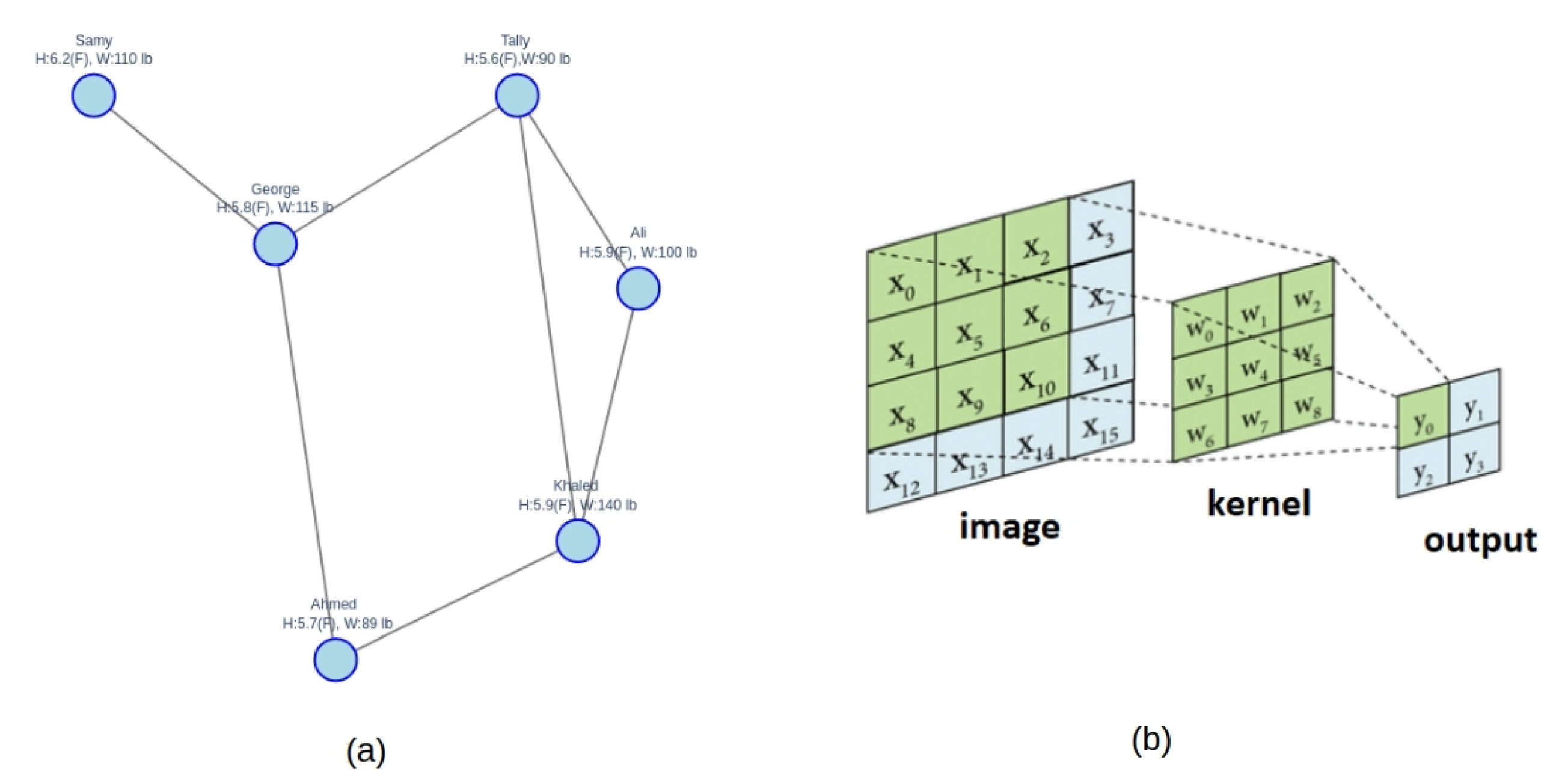
Figure 2.
GCN-MILP Flowchart.
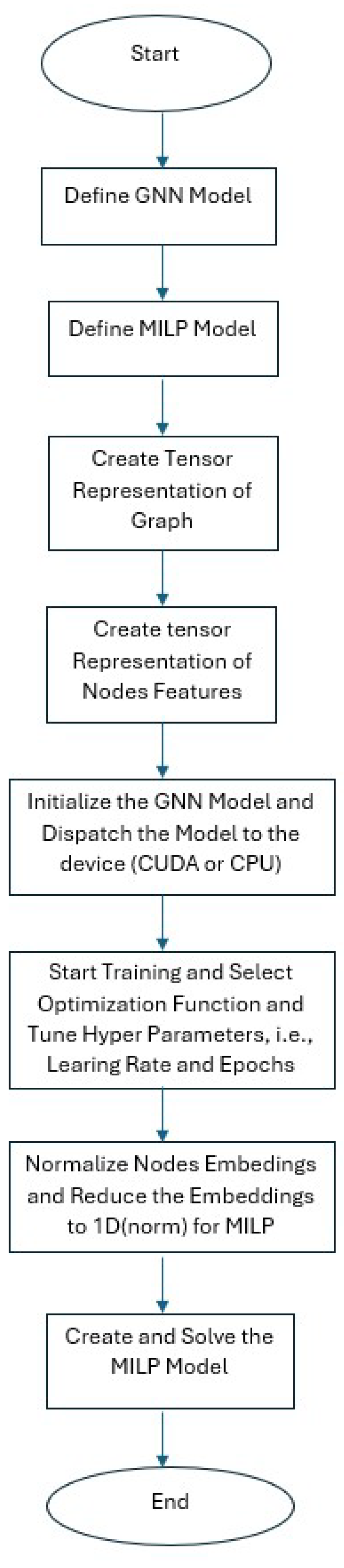
Figure 3.
The proposed GCN-MILP model interaction.
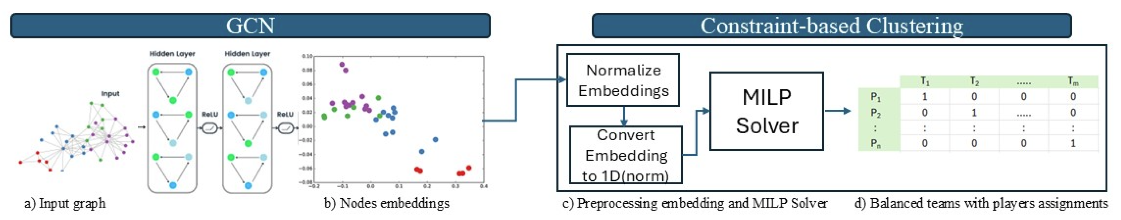
Figure 4.
A sample run where an optimal solution exists.
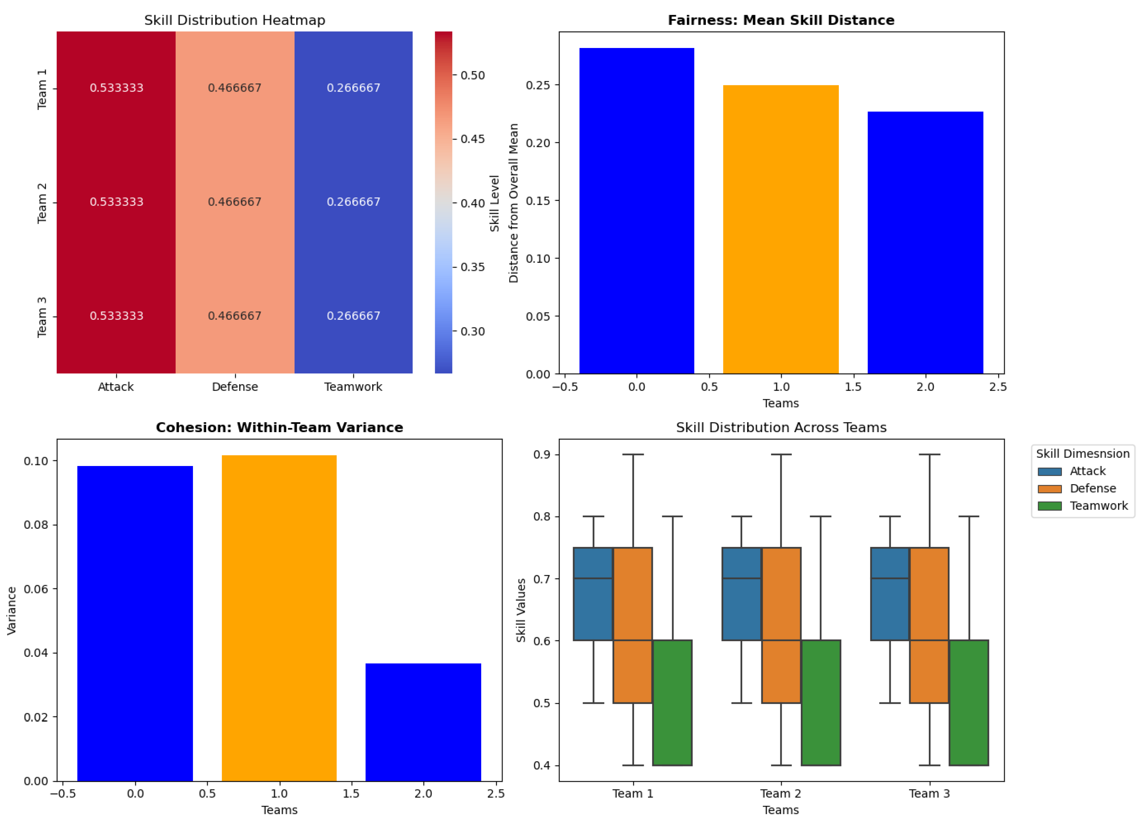

Table 1.
Gini Coeficient.
| Team | Gini Coef. |
|---|---|
| Team 1 | 0.89 |
| Team 2 | 0.89 |
| Team 3 | 0.89 |
Table 2.
Result of Second Experiment.
| Metric | Value |
|---|---|
| Team 1 | [7, 8, 9, 16, 19] |
| Team 2 | [3, 11, 12, 15, 17] |
| Team 3 | [4, 10, 13, 14, 18] |
| Team 4 | [0, 1, 2, 5, 6] |
| Mean Skill Distance | 0.6222 |
| Within-Team Variance | 1.6956 |
| Skill Balance | 0.1052 |
Disclaimer/Publisher’s Note: The statements, opinions and data contained in all publications are solely those of the individual author(s) and contributor(s) and not of MDPI and/or the editor(s). MDPI and/or the editor(s) disclaim responsibility for any injury to people or property resulting from any ideas, methods, instructions or products referred to in the content. |
© 2025 by the authors. Licensee MDPI, Basel, Switzerland. This article is an open access article distributed under the terms and conditions of the Creative Commons Attribution (CC BY) license (http://creativecommons.org/licenses/by/4.0/).
Copyright: This open access article is published under a Creative Commons CC BY 4.0 license, which permit the free download, distribution, and reuse, provided that the author and preprint are cited in any reuse.


