Submitted:
12 January 2025
Posted:
13 January 2025
Read the latest preprint version here
Abstract
This article studies the PDE for the joint probability density function for multi-variate Brownian motions where the correlations are not constant. In particular, with some assumption on the correlation function, this article shows the high dimensional PDE can be decomposed into lower dimensional PDEs which make the calculations fast and stable for practical applications.
Keywords:
Gaussian distribution
; correlation skew
1. Background
Gaussian copula is widely used in quantitative finance modelling. The Gaussian distribution is closely related to an underlying Brownian motion: the standard multi-variate normal distribution is the terminal distribution of an underlying multi-variate Brownian motion where the correlations are constant over time. However the correlation being constant is a limitation of this model which might not fit the actual market. On the other hand, if the correlations are not constant, the result terminal distribution has no closed-form representation in general. Without the closed-form solution or analytic tractability, it becomes less attractive for practical usage. There are research in alternative directions which bypass this tractability issue, for example in [1,2], the respective authors created different terminal distributions which can admit shape with the desired correlation skew effect. In this paper, we still focus on the terminal distribution result from the Brownian motion itself. We study the PDE for the density function and show that with some assumption on the correlation function, the PDE can be decomposed to lower dimensional ones and therefore make the calculation fast and practical. With this technique, the result distribution can be a useful variation to the standard multi-variate normal distribution and it can be used for purpose like modelling correlation skew effect in quant finance.
We also think the terminal distribution with non-constant correlation might be an interesting mathmatical object on itself.
2. Methodology
We study this math problem below. This is a 2-dimensional case however we show later that similar techniques can be applied to higher dimensions.
This is a 2d-PDE in the convention of quant finance industry (2d refers to 2-dimension in space variables while in fact it is a 3-d PDE if counting t, given the common presence of t in this type of PDE we refer the dimensions to only the space variables) and the general numerical method is slow. However, we can decompose the 2d-PDE into two 1d-PDEs if we make a reasonable assumtion on the correlation function as below:
This means the correlation depends on the in terms of the total , which can be interpreted as: correlation depends on a market factor which is the average of the underlyers. With this extra assumption, we can simplify the problem as below:
Lets make change of variables below
Then we have
And can be written as
Note the first equation only involves u, then Fokker-Planck equation for u is a 1d-PDE:
So we can solve first, then we look at the . For any given path , the is simply a sum of infinitesimal normal variables with variances , so we know the distrubtion of condition on this path is a normal distribution with mean 0 and variance
Conditioned on a path is not easy to use for calculation, it would be more useful to condition on a value instead of the whole path. Lets consider the conditional expectation
This is the path integral on all possible paths that get to u at t. We have the following:
The is the transition probability from state to .
Now we follow the Fokker-Planck equation derivation technique, we will get:
The proof is standard derivation, readers can skip it. For completeness we include the outline below:
Outline of proof:
Note the second term comes to
So we just have to prove
Let be a smooth function with compact support, consider
Now the integral is the moment of the Brownian motion , so we have
Then we have below, in the order of
so
The last step in above is integration by parts. Because the is arbitrary smooth function so it follows that:
End of Proof.
To recap, we have these 2 key equations:
We can solve for p first and then solve for f (It is also possible to bundle the PDE solving for p and f together in discretization etc). Knowing and , the whole distribution is known. The key point here is when solving p or f it is a low dimension PDE.
3. Higher Dimensions
In higher dimensions, similar technique can be applied if we assume the correlations have a dependency on one variable (though the variable might be defined as a linear combination of the base variables) and time only. A brief walk through of the idea as below:
Let be the initial Brownian motion variables with correlations . For simplicity and avoid any singularity questions, lets assume the all just depend on variable and t. Now we can represent the random process by new set variables , ( is left out as it can be implied by others). We can do Cholesky decomposition of this set of variables and a nice property is that the Cholesky matrix elements are all just function of M and t: this is because all the are just function of M and t and the Cholesky decomposition is a deterministic operation on those . Now we can apply the same process as before, solve for the probability density of M, and then for variance function of each of the independent Brownian motion variables coming from the Cholesky decomposition. The process will be long and tedious but there is no conceptional difference to the previous case. Note in a special case where all the are the same function, the change of variables is much cleaner and easier.
So in general, with the assumption that the correlation dependency degenerated to one variable only, the joint terminal distribution of dimension n can be calculated by n 1-d PDEs (1-d refer to 1 space variable).
4. Implementaion Example
We show one example of 2-d case: We discretize p and f together and solve for p first for a time step, and then solve for f. We don’t use chain rule to break out the partial derivatives of product but instead discretize on the product. With standard finite difference methods, the calculation is fast and stable. We present an example of the distribution below:
Figure 1 shows the contour of a Gaussian distribution with correlation skew. The underlying correlation function is:
The graph axis is in x and y. Note will be the two diagonal directions.
The shape of the contour is expected. As we put higher correltion when the is lower, and lower correlation when u is higher, the probability is more concentrated when u is low and more dispersed when u is high. Note with u fixed, the graph also shows symmetry in the direction of v.
The following graphs shows more details on in above example.
In Figure 2 the distribution of u is very close but different to a standard normal. To see the difference, we reflected the probability around center and then one can see the negative part has a fatter tail than positive part. This is expected as we correlated more when is more negative, we expect will have more potential to go lower in the negative direction, and as we de-correlate more when more positive, we expect the diversifying effect makes the less potential to go higher when positive.
To demonstrate this point, we can increase the skew of correlation further to see the fat tail effect. Below is the for a more skewed correlation function.
The correlation function in Figure 3 is
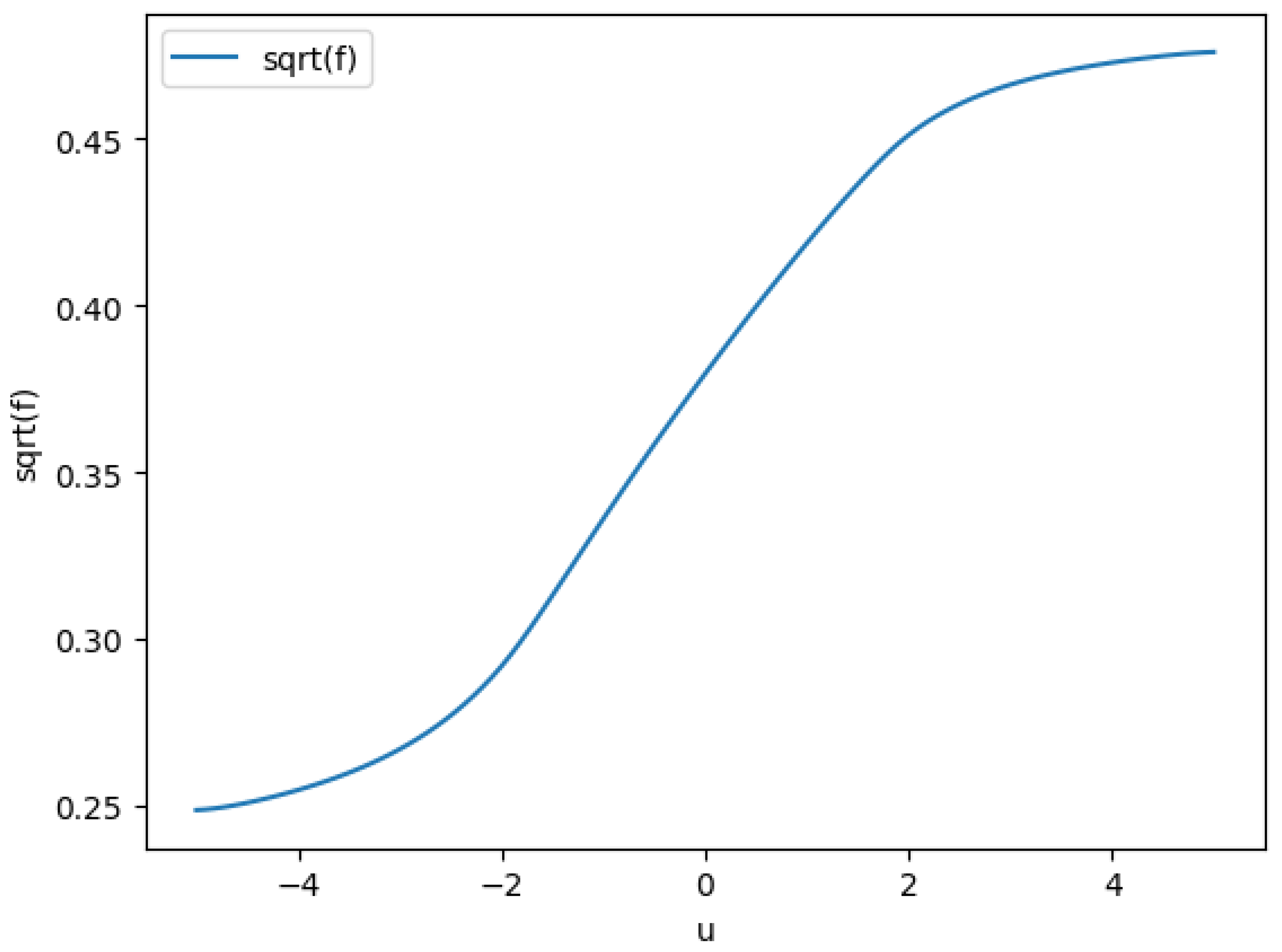
The coutour in Figure 1 shows the v is concentrated when u more negative and v is spreaded when u is more positive.
5. Copula Application
Knowing the and we can integrate any function on this terminal distribution. For given , it maps to , and the marginal distribution of x and y are still normal distribution respectively, so they can be readily used to invert CDFs.
References
- Fokker, A. D. Die mittlere energie rotierender elektrischer dipole im strahlungsfeld. Annalen der Physik 1914, 348, 810–820. [Google Scholar] [CrossRef]
- Kolmogorov, A. Uber die analytischen methoden in der wahrscheinlichkeitstheorie. Math Annal 1931, 104, 415–458. [Google Scholar] [CrossRef]
- Lucic, V. (2012). Correlation skew via product copula. In Financial engineering workshop, cass business school.
- Luj´an, I. Pricing the correlation skew with normal mean–variance mixture copulas. Journal of Computational Finance 2022, 26. [Google Scholar]
- Planck, V. (1917). ¨Uber einen satz der statistischen dynamik und seine erweiterung in der quantentheorie. Sitzungberichte der.
Figure 1.
Contour of Gaussian distribution with correlation skew
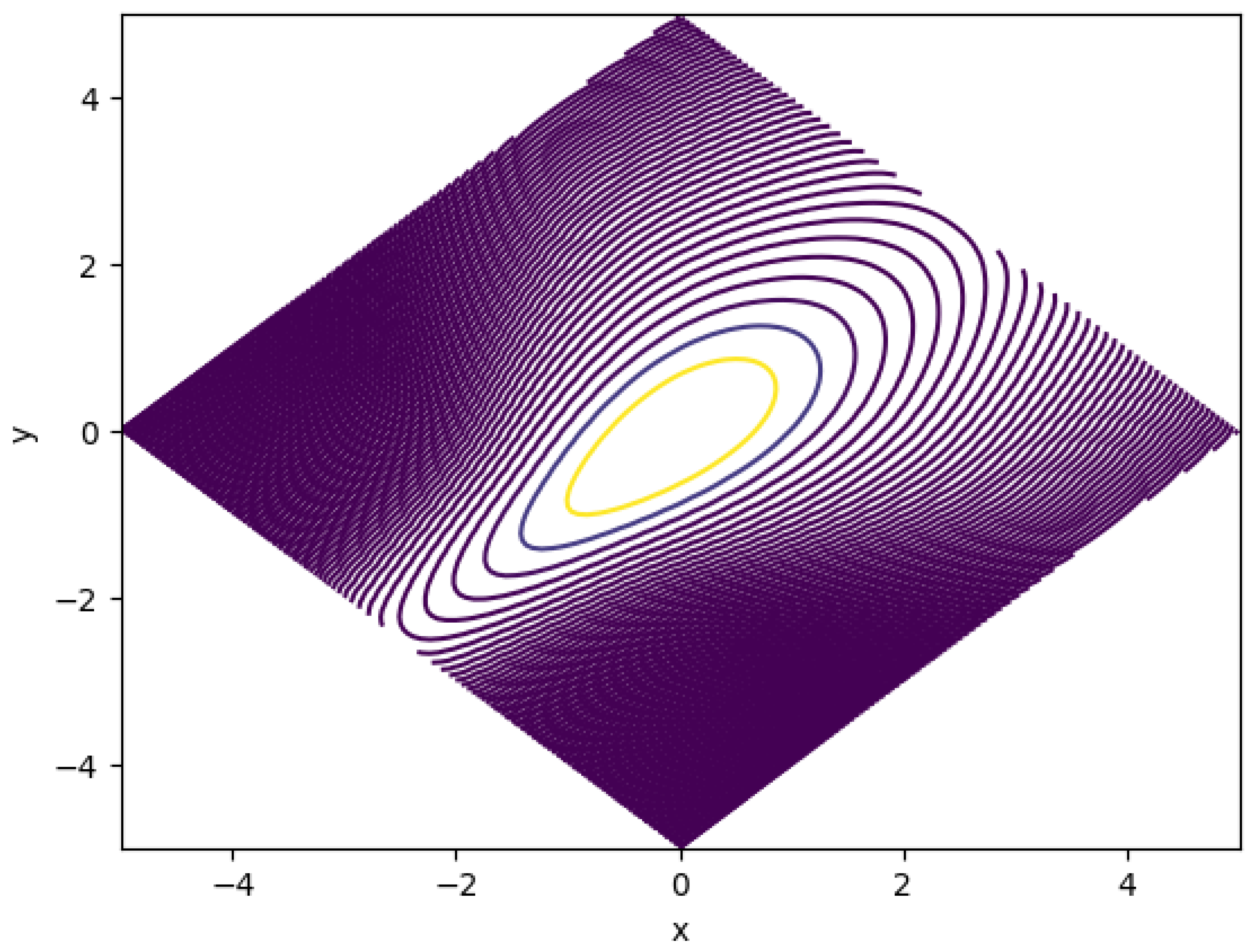
Figure 2.
Marginal distribution of u
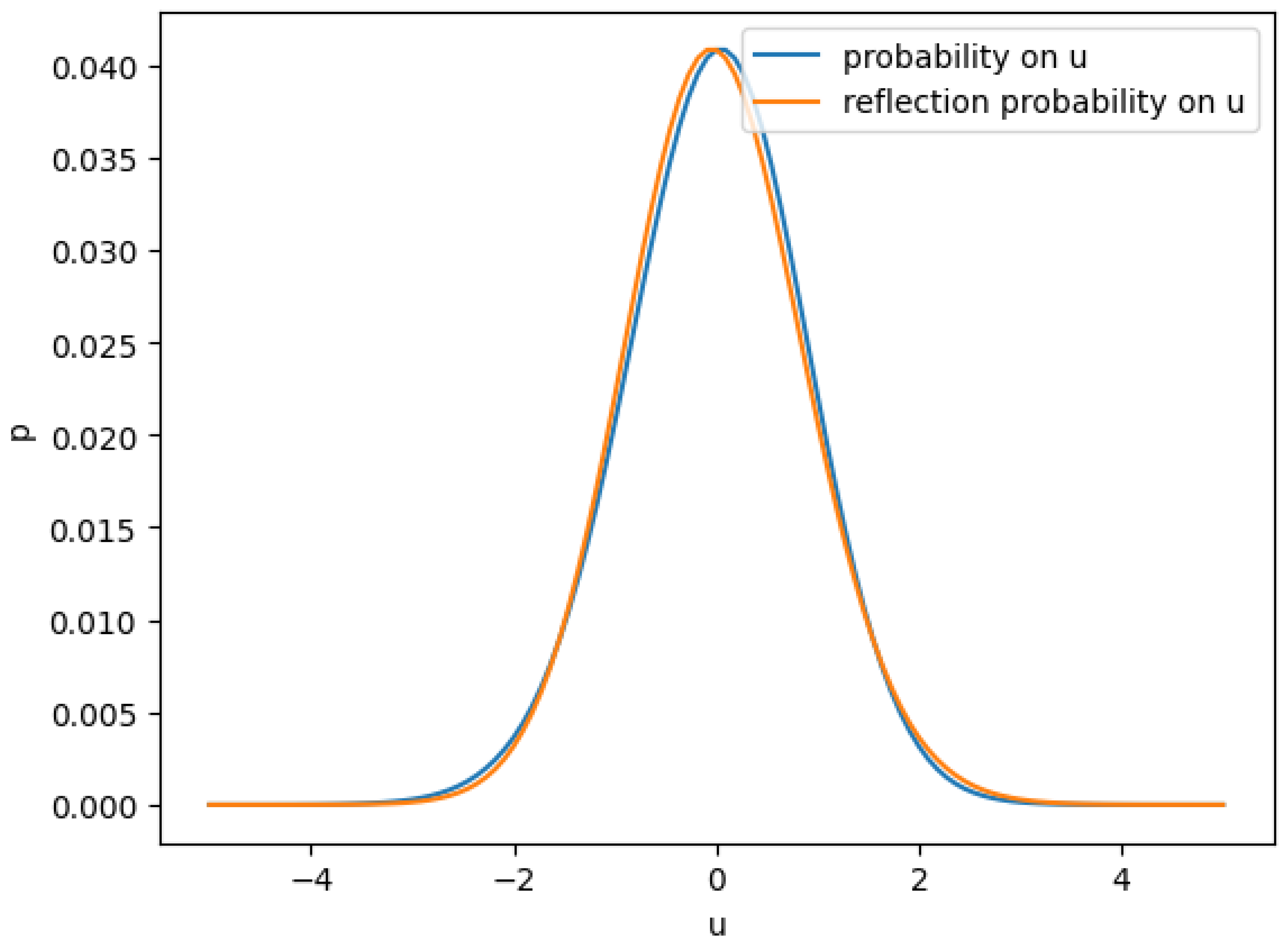
Figure 3.
Marginal distribution of u
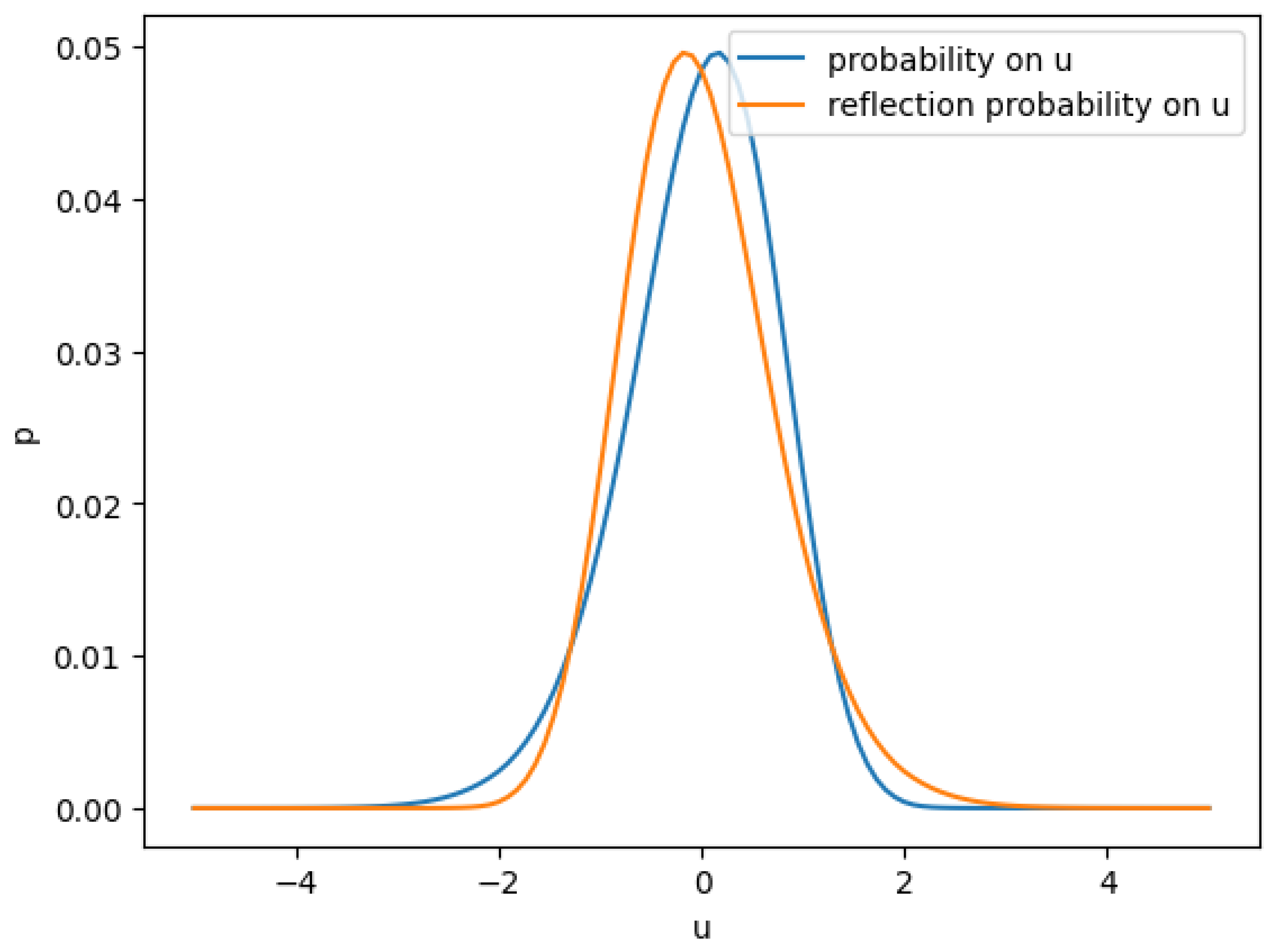
Figure 4.
std dev of v conditioned on u
Disclaimer/Publisher’s Note: The statements, opinions and data contained in all publications are solely those of the individual author(s) and contributor(s) and not of MDPI and/or the editor(s). MDPI and/or the editor(s) disclaim responsibility for any injury to people or property resulting from any ideas, methods, instructions or products referred to in the content. |
© 2025 by the authors. Licensee MDPI, Basel, Switzerland. This article is an open access article distributed under the terms and conditions of the Creative Commons Attribution (CC BY) license (http://creativecommons.org/licenses/by/4.0/).
Copyright: This open access article is published under a Creative Commons CC BY 4.0 license, which permit the free download, distribution, and reuse, provided that the author and preprint are cited in any reuse.


