1. Introduction
Arid regions constitute approximately 20% of the Earth’s terrestrial surface and are among the ecosystems most vulnerable to climate change (Lian et al. 2021). As the largest country under threat of desertification (Guo et al. 2022), China features decertified land spanning over 2.6 million km2, accounting for 27% of the whole territory (Ren et al. 2024). These areas are predominantly located in extremely arid, arid, and semiarid zones, where water resources are critically scarce (Wei et al. 2021).
The scientific reclamation of desert areas is a primary strategy to mitigate desertification and has been widely implemented in arid regions (Ma et al. 2024). While the natural weathering of soil is a prolonged process, conventional and conservation tillage practices significantly influence soil microstructure, moisture and thermal dynamics, nutrient content, and the composition of soil organic matter. These practices collectively improve soil quality in newly reclaimed cultivated land (Liu et al. 2021; Man et al. 2021). Numerous studies have demonstrated the positive impact of reclamation on desert soil quality. Firstly, reclamation reduces the risk of soil degradation and enhances resistance to wind erosion (Fallahzade et al. 2020). Secondly, it improves the physical properties of desert soil by decreasing bulk density and increasing the proportions of clay and silt particles, as well as soil organic carbon (SOC) levels. These changes enhance the soil’s ability to retain nutrients and water (Cao et al. 2021; Shang et al. 2019). Lastly, short-term agricultural activities following reclamation stimulate soil microbial activity and significantly increase nitrogen (N), phosphorus (P), and other nutrient levels (Chen et al. 2020; F.-R. Li et al. 2018). However, soil quality improvements from reclamation are not indefinite. According to Hua et al. (2008), desert soils stabilize 6–8 years after reclamation, and soil quality often begins to decline after 10 years. Furthermore, the long-term effects of reclamation, particularly for pure desert soils, remain uncertain. Most existing studies focus on semi-shrubby deserts, grasslands, and oasis forests in regions with limited agricultural histories, suggesting that at least 50 years may be required for desert soils to transform into highly productive agricultural land (Su et al. 2010). Short-term observations may fail to capture the slow and complex processes of soil evolution, obscuring the long-term trends following reclamation (Bacq-Labreuil et al. 2021; Ma et al. 2024).
Arid and semiarid regions are particularly vulnerable to desertification due to low and highly variable precipitation, high evaporation rates, nutrient-poor soils, sparse vegetation, and fragile ecosystems (Maestre et al. 2021). These regions also feature saline soils with low moisture content and extremely high electrical conductivity (Hachmi et al. 2018; Mihi et al. 2019). Such physicochemical constraints limit the transformation rate of organic matter, leading to the accumulation of untransformed materials. This phenomenon negatively affects soil fertility, impeding the recycling of essential nutrients required for plant growth (Hall et al. 2011; Sinsabaugh et al. 2009; Y. P. Wang et al. 2010). Given these complexities, research focusing on long-term agricultural chronologies is essential to comprehensively understand the impact of desert reclamation on soil properties and to discern the gradual evolution patterns of reclaimed desert soils.
Few studies have focused on subsoil in arid regions due to its limited development and low particle cohesion, which complicate the application of conventional investigative methods. In this context, digital soil mapping (DSM) offers a promising alternative for predicting the three-dimensional distribution of various soil properties. Over the past two decades, DSM techniques have gained significant traction for identifying spatial soil patterns and their associated characteristics (McBratney et al. 2003; Minasny and McBratney 2016; Poggio et al. 2021). Among these techniques, machine learning algorithms have become increasingly popular due to their capacity to model complex interactions between soil properties and environmental variables with high accuracy, particularly when applied to large soil datasets (Arrouays et al. 2020; Heuvelink and Webster 2022). Several studies have shown that machine learning techniques can accurately predict SOC at various scales and in a variety of ecosystems, including semiarid and arid regions (Wiesmeier et al. 2011; Zeraatpisheh et al. 2019). These DSM products are essential for enhancing soil management and conservation strategies, particularly given the vulnerability of semiarid regions to climate change and anthropogenic pressures (Azamat et al. 2024). Moreover, soils exhibit significant temporal and spatial variability, necessitating an investigation of vertical distributions of soil properties (Poggio and Gimona 2014). Each soil property follows a unique vertical distribution pattern, varying continuously with depth within the profile. These patterns can be modeled using depth functions, which have evolved from the freehand curves pioneered by(Bishop et al. 1999; Jenny 1941)) to more sophisticated mathematical models. Examples include polynomial functions, power functions, equal-area quadratic spline functions (EAQSFs) (Bishop et al. 1999), exponential decay functions (EDFs) (Minasny 2006), and sigmoid functions (Y. Zhang et al. 2017).
When combined with machine learning algorithms, these depth functions have proven effective in modeling the three-dimensional distribution of soil properties, as demonstrated by studies on SOC (Allory et al. 2022; Fu et al. 2024). However, research on other soil properties, particularly in arid and semiarid regions, remains limited. Therefore, further investigation is urgently needed to evaluate and optimize the performance of existing modeling approaches for predicting a broader range of soil properties in these challenging environments.
In this study, a variety of soil properties were selected. Through correlation analysis, four soil properties, SOC, TP, NH4+ and pH, were ultimately identified as the most critical soil properties. These properties were selected to elucidate the variation trends with depth and their spatial distribution characteristics, providing insights into the effects of semicentennial tillage on soil evolution. To determine the best approach for predicting soil properties in the study area in Xinjiang Province, Northwest China, three machine learning models—the multiple linear regression (MLR), quantile regression forest (QRF), and boosted regression tree (BRT) methods—combined with various depth functions were investigated. The objectives of this study were to (1) predicting and comparing the spatial distributions of soil properties (SOC, TP, NH4+ and pH) via various DSM approaches, and (2) verify the impact of semicentennial desert reclamation on soil properties and soil evolution.
2. Materials and Methods
2.1. Description of the Study Area
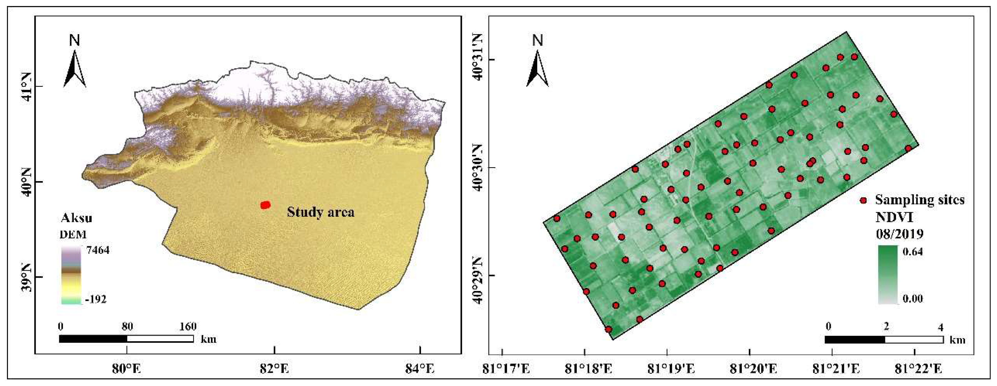
The study area is situated in southern Xinjiang, China (81°17′–81°22′ E, 40°28′–40°31′ N) (
Figure 1), at the confluence of the Hetian, Aksu, and Yerqiang Rivers. It lies north of the Tarim River and south of the Taklimakan Desert. The region experiences high annual sunshine exposure, with a mean duration of 2303.1 hours. Due to its arid climate, characterized by low precipitation (mean annual precipitation of 60 mm) and high evapotranspiration (1800 mm), substantial amounts of water from the Tarim River have historically been utilized to reclaim desert land and establish oasis agriculture, beginning with the founding of Aral City. Over time, the city’s reclaimed cultivated land has continued to expand, and the desert edge has continued to move towards the south. However, the effects of this reclamation on the three-dimensional distributions of the critical soil properties in this area are unknown.
2.2. Experimental Design and Soil Sampling
We selected the 12th Regiment farm, which has been cultivated in natural sandy lands for more than 50 years; additionally, six adjacent, noncultivated virgin sandy land sites served as a reference (control). Previous studies in this area revealed that the soil properties in the cropland areas before cultivation were similar to those in the adjacent uncultivated sandy areas.
In August 2019, 71 sampling sites were distributed via a regular grid layout on the farm, with intervals of 1 km from east to west and 500 m from north to south. Each sampling site was drilled to a depth of 1 m, and two soil samples from 0–10 cm, 10–20 cm, 20–40 cm, 40–60 cm, 60–80 cm and 80–100 cm were collected. The soil samples from the same level at different drilling points were mixed, and visible roots and litter debris were removed from each soil sample. Finally, the samples were air dried and sieved through a 2 mm soil sieve for physicochemical analysis.
2.3. Analysis of Soil Physical and Chemical Properties
The pH of the air-dried soil was determined by extracting 5 g of soil with 0.01 M CaCl2 (1:5) in an end-over-end shaker for 1 h followed by centrifugation at 492 × g for 10 min. The pH of the supernatant was determined via a Thermo Orion pH meter (Thermo Orion 720A+, Beverly, MA, USA). The soil organic carbon (SOC) content was determined via the K2Cr2O7-H2SO4 oxidation method of Walkley-Black (Nelson and Sommers 1982). The total phosphorus (TP) content was determined calorimetrically after wet digestion with H2SO4-HClO4 (Parkinson and Allen 1975). Ammonium-N (NH4+) was determined with an AA3 Continuous Flow Analytical System (Bran+Luebbe, Norderstedt, Germany) following extractions of fresh soil with 1 mol L−1 KCl.
Notably, several soil properties, including TN, TK, and CEC, were selected. We carried out correlation analysis on all these soil properties and selected the four with the lowest correlation.
2.4. Environmental Covariates
One of the primary elements influencing the formation of soil in arid and semiarid areas is topography (Zeraatpisheh et al. 2019). A digital elevation model (DEM) with a cell size of 12.5 m x 12.5 m was thus downloaded from ALOS PALSAR in order to obtain the topographic attributes (“ASF Data Search” n.d.). Elevation (El), topographic wetness index (TWI), slope (SL), slope position (Slpposi), profile curvature (PrCu), plan curvature (PlCu) and distance to an irrigation canal (DIC) were among the terrain variables derived from the DEM.
The normalized difference vegetation index (NDVI), carbonate index (CAEX) and salinity index (SI) were among the auxiliary variables used in remote sensing. The environmental covariates were obtained using the SAGA GIS (System for Automated Geoscientific Analysis), and predictors with varying resolutions were resampled to 10 m using the bilinear interpolation approach.
2.5. Modeling Approaches
Two nonlinear machine learning models, namely, QRF, BRT, and MLR, combined with different depth functions, such as exponential functions, logarithmic functions, power functions and cubic polynomial functions, were used for the digital mapping of soil properties (SOC, TP, NH4+ and pH).
BRT analysis is a parametric data mining technique that can handle both nonlinear and linear relationships (Myles et al. 2004), and it has been reported that this technique has been widely used in the field of DSM (Taghizadeh-Mehrjardi et al. 2014).
A regression forest (RF) is a classifier or regression model made up of numerous decision or regression trees, each of which is reliant on the values of a randomly selected vector that is sampled separately and has the same distribution as all the other trees in the data. (Liaw and Wiener 2002). (Meinshausen n.d.) suggested altering the RF procedure’s outputs by permitting the calculation of the targeted variables’ prediction intervals. The QRF technique takes into account the spread of the response variable from which prediction intervals are formed, whereas the RF technique merely preserves the mean of the observations that fall into each node and ignores all other information for each node and each tree.
Spatial prediction has long employed linear regression, one of the first statistical methods (Draper and Smith 1998). Multiple linear regression fits the data to a straight line (or plane in an n-dimensional space, where n is the number of independent variables) (Mbagwu and Abeh 1998). As a result, each soil property has been given a quantitative estimate using the MLR model.
Pearson correlation coefficients between the environmental covariates and soil parameters were computed in order to identify significant environmental covariates. Each soil attribute was then predicted using only relevant factors (Aksoy 2012). Based on variable relevance, the most significant variables were determined for each model. In many applied models, the quantification of variable importance is a crucial topic (Genuer et al. 2010). It helps in the interpretation of the variables and their impact on model correctness (Genuer et al. 2010) as well as the identification of the most significant environmental covariates utilized in the models (Nauman and Thompson 2014). The “caret” package in R 4.3.3 and RStudio was used for all modeling and variable significance computations.
2.6. Statistical and Validation Strategy
Leave-one-out cross-validation (LOOCV) was performed to evaluate the prediction methods. In order to ensure that every data point appears in the test set at least once, cross-validation offers a framework for generating multiple training/test splits in the dataset. This approach has the benefit of impartiality and consistent performance on smaller datasets.
The model performance was assessed using three validation criteria: the coefficient of determination (R
2), the mean absolute error (MAE), and the root mean square error (RMSE).
where P
i, O
i, O
avg, P
avg,
n, and
p stand for the model’s total number of explanatory variables, number of data points, average of the observed and predicted soil property values at the ith point, and predicted and observed values, respectively.
3. Results and Discussion
3.1. Correlation Analysis and Descriptive Statistics
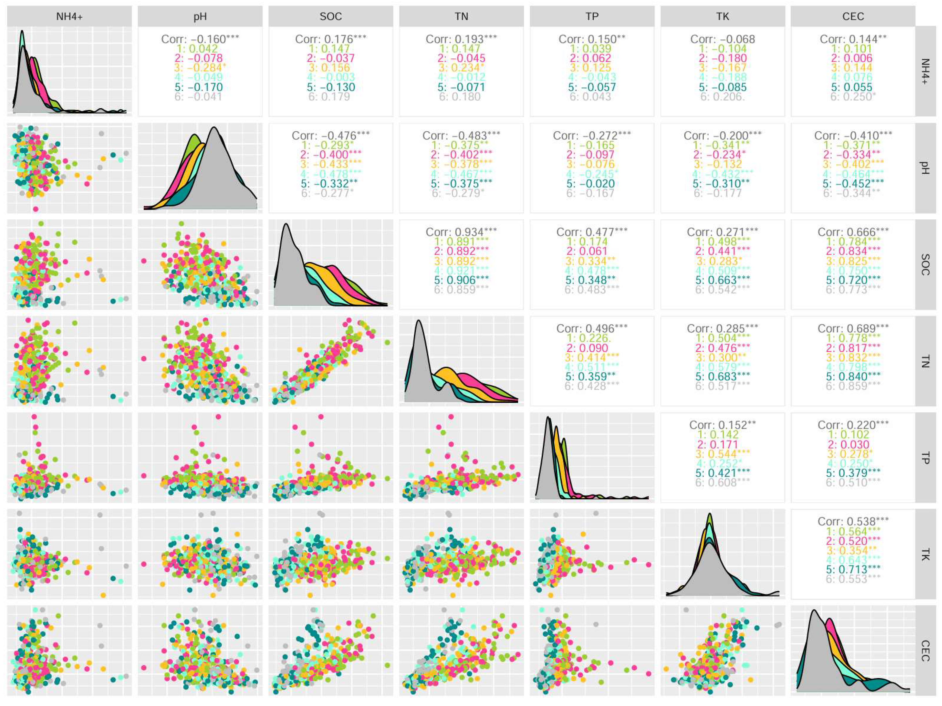
We measured a variety of properties and selected four soil properties, SOC, pH, NH
4+ and TP, which are related to other soil properties, but their correlations with each other are low (
Figure 2). The soil properties not selected, such as TN and SOC (r = 0.93), CEC and SOC (r = 0.67), and TK and CEC (r =0.54), were highly correlated with the four selected soil properties. In this way, we ensured the maximum representativeness and heterogeneity of the selected attributes.
The summary statistics of the soil properties in the study area are presented in
Table 1, while those of the CK are presented in
Table 2. Scatter diagrams of SOC, pH, NH
4+ and TP are shown in
Figure 4. Notably, we removed the ten maximum values and ten minimum values from each layer for the sake of aesthetic considerations and to ensure that these depth functions were distinguished to the greatest extent. In the study area
, the mean values and standard deviations of the SOC content decreased with depth, and the mean values were 4.49, 4.19, 3.61, 2.69, 2.31 and 2.19 g/kg, respectively. The coefficients of variation (COVs) of the SOC content at the 0–20 cm depth were less than 35%, indicating moderate variation, and those at the 20–100 cm depth ranged from 35% to 43%, indicating high variation. The mean values of pH increased with increasing soil depth and were 8.83, 8.86, 8.91, 8.99, 9.02 and 9.07. The COVs of the pH values at the six depths ranged from 2.54% to 3.11%, indicating low variation. The mean values of NH
4+ increased with depth from 0–50 cm and then decreased with depth from 50–100 cm, with values of 3.06, 2.80, 2.43, 2.07, 2.33 and 2.48 mg/kg, respectively. The COVs of the NH
4+ content at the 0–20 cm depth were less than 35%, indicating moderate variation, and those at the 20–100 cm depth ranged from 35% to 62%, indicating high variation. The mean values and standard deviations of the TP content decreased with depth, and the mean values were 1.04, 1.05, 0.90, 0.78, 0.71 and 0.70 g/kg, respectively. The COVs of the TP content at depths of 0–20
cm were less than 35%, indicating moderate variation, and those at depths of 20–100 cm were less than 25%, indicating little variation.
In the CK treatment, there was no significant trend in the values of SOC, pH, NH
4+ and TP with increasing depth. We plotted the changes in the values of the four soil properties at different depths after semicentennial tillage, as shown in
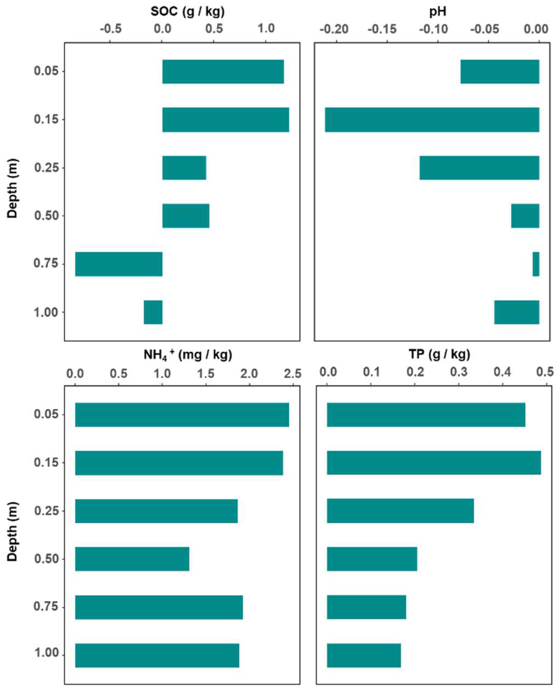
Figure 3, which revealed the vertical changes in the soil properties following semicentennial tillage in desert areas. The observations revealed that the accumulation of SOC is higher than that of the CK at 0–60 cm but lower in the 60-100 cm layer. Additionally, the pH of the reclaimed soils was lower than that of the CK soils, while the NH
4+ and TP contents were greater than those of the CK soils in both the topsoil and subsoil. These findings indicate that reclamation has led to increases in N and P contents. Although reclamation promoted an increase in SOC in the subsoil, it also resulted in a decline in the SOC accumulation rate within this layer; notably, this rate decreased with increasing depth.
Figure 3.
Histograms of the SOC, pH, NH4+ and TP values in the experimental group (TG) minus the control group (CK).
Figure 3.
Histograms of the SOC, pH, NH4+ and TP values in the experimental group (TG) minus the control group (CK).
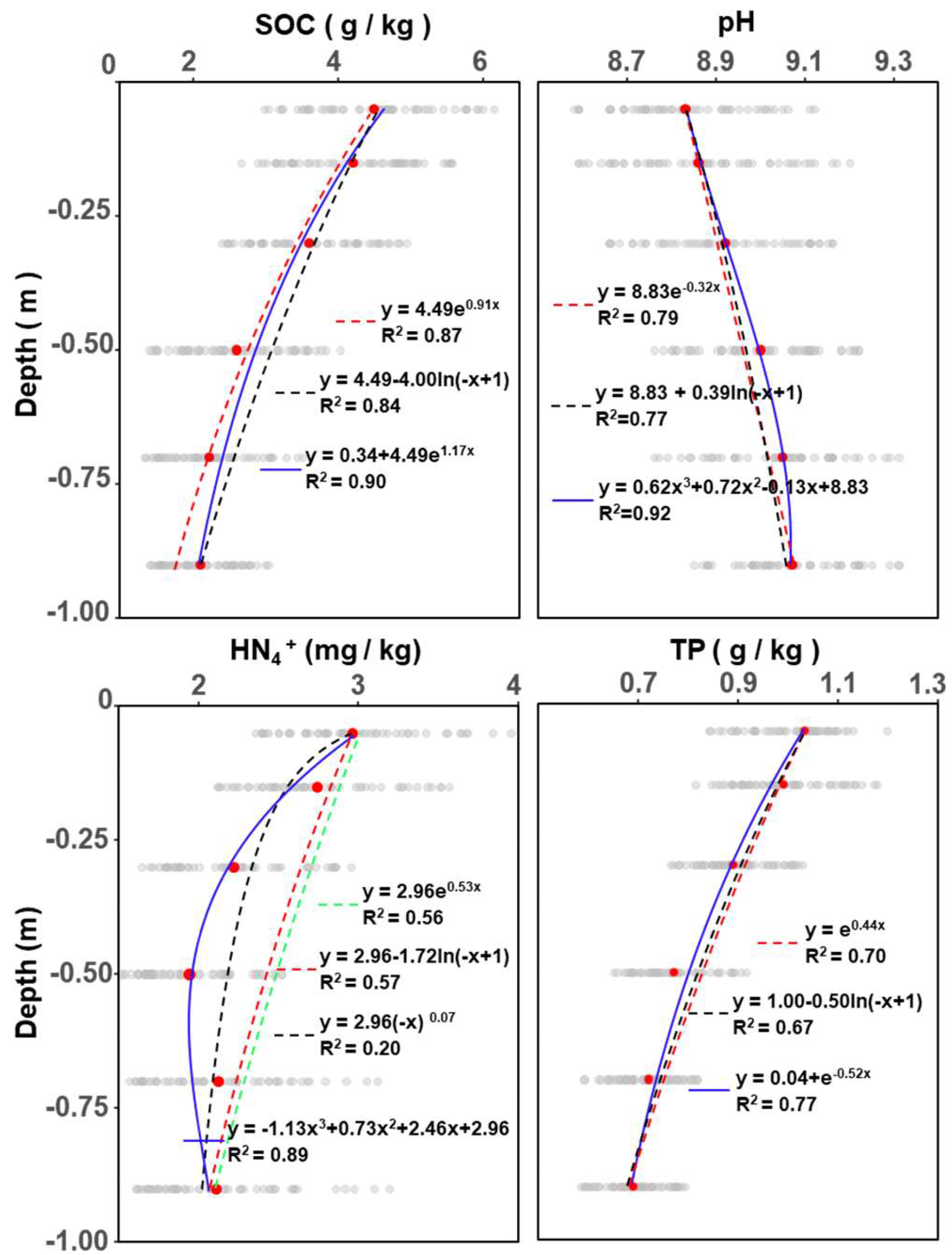
Figure 4.
Fitted vertical distributions of SOC, pH, NH4+ and TP. The red circles indicate the mean values of SOC, pH, NH4+ and TP in each layer. All the presented formulas are inverse functions.
Figure 4.
Fitted vertical distributions of SOC, pH, NH4+ and TP. The red circles indicate the mean values of SOC, pH, NH4+ and TP in each layer. All the presented formulas are inverse functions.
In arid and semiarid regions, nutrient accumulation occurs primarily through artificial means. The unique natural characteristics of these areas, particularly the ratio of evaporation to precipitation, pose challenges for the accumulation of essential nutrients such as C, N, and P, which are necessary for the growth of plants (Gamalero et al. 2020).
The contents of SOC are determined primarily by the balance between exogenous crop carbon inputs and the decomposition of existing SOC (F. Zhang et al. 2022). In arid and semiarid regions, differences in temperature between the topsoil and subsoil affect microbial activity, which subsequently influences SOC mineralization at different depths (X. Li et al. 2020; C. Wang et al. 2021; Yu et al. 2022). After reclamation, topsoil has a relatively high clay content that facilitates the formation of mineral-associated organic carbon compounds (Song et al. 2024). The minimal variation observed in SOC at different depths in the CK can be attributed to the high and uniform sand content.
The reduced levels of SOC in the 60–100 cm layer relative to those in the CK soil can be explained by the evaporation rate exceeding the precipitation rate, which limited the downwards migration of soluble organic carbon. The study area is located on the northern edge of the Taklimakan Desert and is characterized by scarce precipitation and rapid evaporation. This environment has led to a gradual accumulation of alkaline ions and soluble salts (Peng et al. 2024). The low vegetation cover results in minimal root activity, which adversely affects the decomposition of organic matter. Cotton, a tap-rooted crop, possesses a main root that can extend to depths of 1–2 m; however, its numerous lateral roots are primarily concentrated within the 0.2–0.6 m range (Kang et al. 2021; Z. Zhang et al. 2020). These lateral roots play crucial roles in promoting SOC decomposition and reducing soil alkalinity, thereby contributing to differences in pH between the 20–60 cm and 60–100 cm soil depths.
NH4+ and TP are both essential nutrients; however, natural processes in desert soils are insufficient for their effective accumulation. In addition to precipitation and evaporation, other soil activities exert minimal influence on the distribution of these nutrients (Shao et al. 2022), which accounts for the limited variation in NH4+ and TP across the CK, with both nutrients showing relatively low concentrations. A high rate of evaporation compared to precipitation typically leads to elevated concentrations of soluble ions in the topsoil relative to the subsoil. However, the lack of significant depth variation in NH4+ and TP in the CK soil may be attributed to moderate rainfall occurring two days prior to sampling. After reclamation, although the surface clay content increased, the soils predominantly retained sandy textures in the profile.
Following irrigation and fertilization, NH4+ was evenly distributed across various soil depths due to water movement. Conversely, phosphorus remains concentrated at or near the surface layer owing to its strong adsorption properties and low solubility, which tend to bind tightly with soil particles. Additionally, under alkaline conditions, phosphate ions readily form insoluble calcium phosphates with calcium ions (Geng et al. 2022; Luo et al. 2023; Yahaya et al. 2023).
3.2. Optimal Depth Functions Selection
Under normal circumstances, there is little difference in the vertical distribution of desert soil properties, whereas watering and fertilization under cultivation produce a series of effects. Consequently, semicentennial tillage is expected to have a longer and more lasting effect on the vertical distribution of desert soil properties. To demonstrate these changes, we used depth functions to simulate the variation trend of desert soil properties with depth after
semicentennial tillage. SOC, pH, NH
4+ and TP within 1 m were fitted by different depth functions, including the exponential function, power function, logarithmic function and cubic polynomial function. The results revealed that different function types had significantly different fitting effects for each soil property (
Table 3 and
Figure 4). The binomial exponential function had the best fitting effect for SOC (R
2=0.90) and TP (R
2=0.77), and the cubic equation had the best fitting effect for pH (R
2=0.92) and NH
4+ (R
2=0.89). These results showed that
semicentennial tillage strongly changed the vertical distribution of critical soil properties and transformed the uniform distribution of desert soil properties from topsoil to subsoil, which may affect soil evolution.
3.3. Model Performance
Semicentennial tillage tremendously changed the soil properties in the study area, not only in the soil profiles but also in different regions, and these changes might have different rates with increasing depth. Two nonlinear machine learning models, namely, QRF and BRT, and a linear model, namely, MLR, were used to predict the distributions of the four soil properties. The performances of the models were evaluated via leave-one-out cross-validation (
Table 4). On the basis of the validation criteria, the nonlinear models (QRF and BRT) were more accurate than MLR. The findings demonstrated that the QRF and BRT techniques performed the best in predicting every property among the models under study.
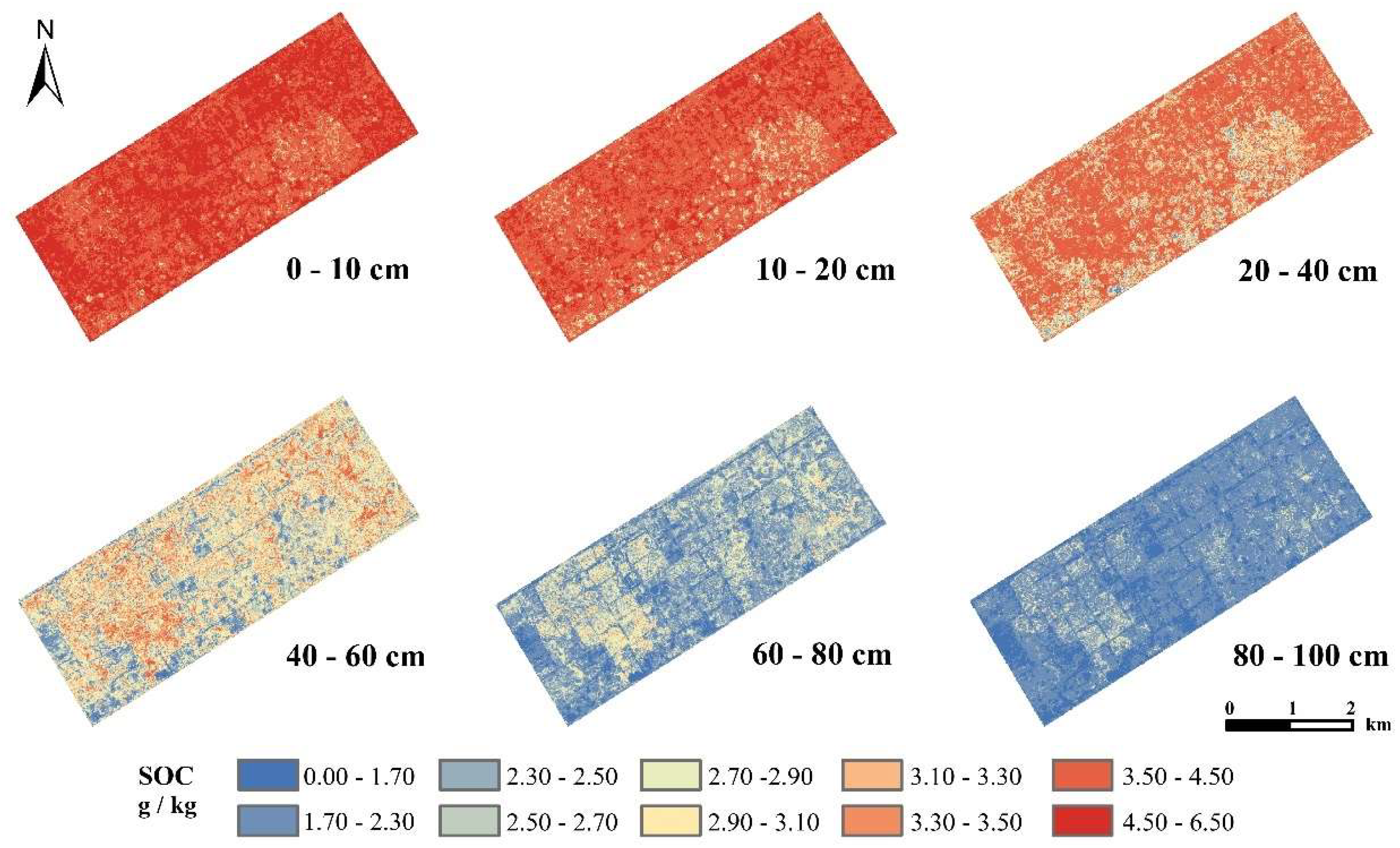
The overall trends of the SOC distribution at the six depths were significantly different, with a spatial pattern of low values in the southeast and west and high values in the middle and north at depths of 0–40 cm. At depths of 40–100 cm, the spatial distribution pattern is characterized by high values in the southeast and west and low values in the middle and north, which was completely opposite to the predicted results for the surface layer (
Figure 5).
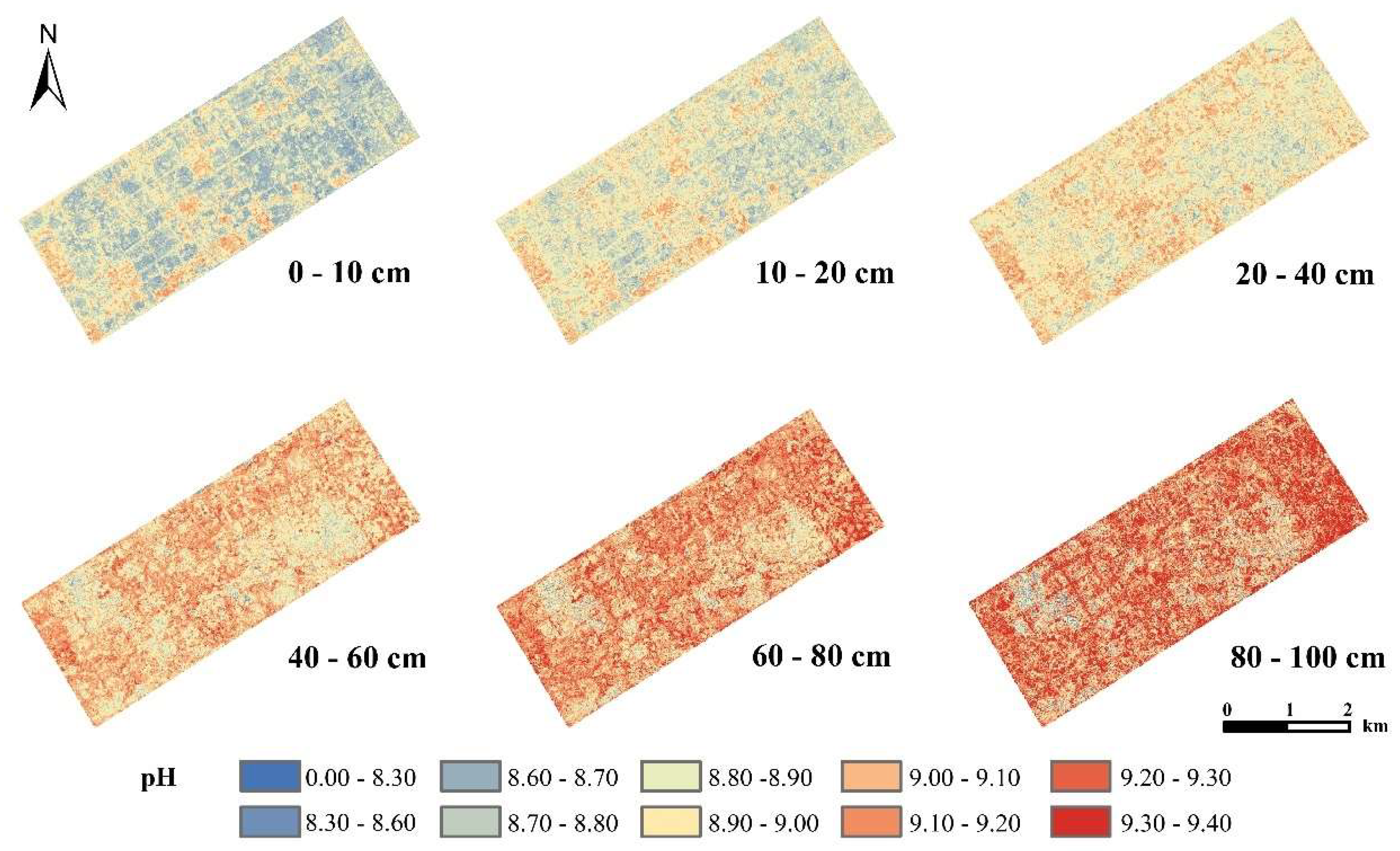
The overall variation trends of the spatial distributions of pH at the six depths were obviously different, and the pH was generally low at depths of 0–20 cm, roughly following the distribution characteristics of farmland. At depths of 20–100 cm, the spatial distribution pattern is characterized by low values in the southeast and west and high values in the middle and north (
Figure 6).
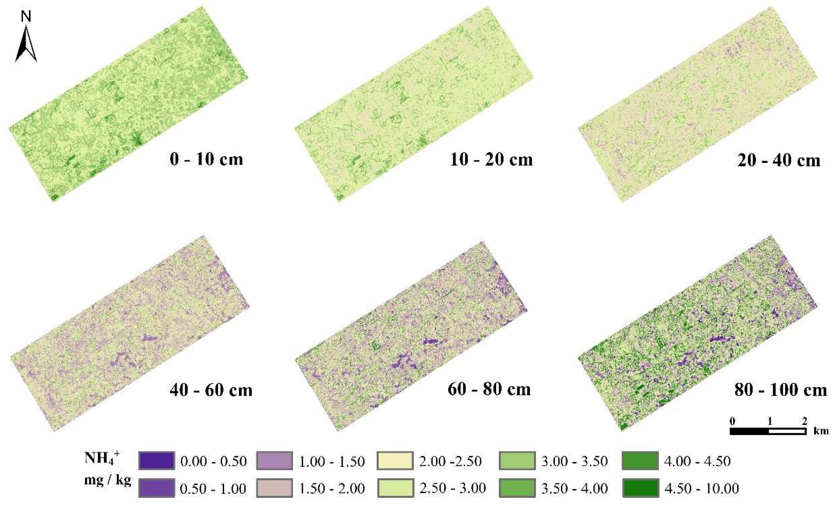
There was no significant difference in the overall trend in the NH
4+ spatial distribution at the six depths (
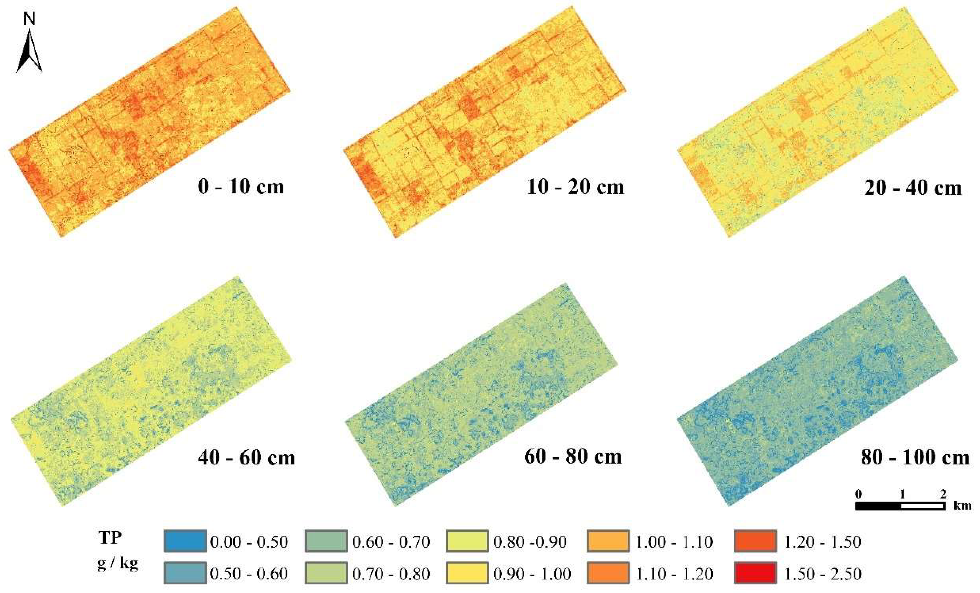
Figure 7). The overall change trend of the spatial distribution of TP at the six depths was consistent, with low values in the southeast and west and high values in the centre and north. The distribution characteristics at 0–40 cm were roughly consistent with those of farmland (
Figure 8).
3.4. Confidence Interval of Prediction
The QRF was used to map the predicted uncertainties. The QRF can be used to estimate the value of a target variable for any required quantile. The upper (95%) and lower (5%) quantile maps can then be used to compute prediction intervals (e.g., 90%). The 5% quantile value indicates that 5% of all possible predictions are lower than this value. This means that under the same conditions, one can predict with 95% confidence that the result will be higher than this value. The 95% quantile value means that 95% of all possible predictions are lower than this value. This means that under the same conditions, one can predict with 5% confidence that the result will be higher than this value. In this study, we used 5% and 95% to represent the confidence interval of prediction (Supplemental Figs. 1-8).
4. Conclusions
Through correlation analysis, this study selected the four soil properties (SOC, pH, NH4+, and TP) with the lowest correlations with each other and high correlations with the properties that were not selected to represent the critical soil properties in the study area. Depth functions were used to assess the variation trends with depth, and nonlinear and linear techniques were used to predict the spatial distributions of SOC, pH, NH4+, and TP. The results showed that the binomial exponential function has the best fitting effect for SOC and TP, and the cubic equation has the best fitting effect for pH and NH4+. The QRF model has the best performance in predicting the SOC, pH, NH4+, and TP contents.
According to the predictions, all critical soil properties changed with depth along the profile, which revealed that semicentennial tillage had a long and lasting effect on the vertical distribution of critical soil properties. In arid and semiarid regions, different temperatures between topsoil and subsoil affect microbial activities, which subsequently influence SOC mineralization at different depths. The clay content, evaporation rate, low vegetation cover and cotton lateral roots played crucial roles in promoting SOC decomposition and reducing soil alkalinity, thereby contributing to variations in the pH between the 20–60 cm and 60–100 cm soil depths. Additionally, under alkaline conditions, phosphate ions readily form insoluble calcium phosphates with calcium ions. Irrigation and fertilization strongly affect the movement of soil water, which results in an even distribution of NH4+. All the changes in soil properties after semicentennial tillage confirmed the occurrence of rapid soil evolution if deserts are cultivated. Thus, desert reclamation was scientifically confirmed to be suitable for agricultural use, which will ease the food production crisis, protect the ecology, and promote soil evolution.
Upon reflection, we conclude that the study area could be expanded, and more chronological observations should be carried out in the expanded area to assess the effects of desert reclamation on soil properties. All of these factors will lead to more precise conclusions and provide more specific guidance for local agricultural development.
Funding
The research was financially supported by the National Natural Science Foundation of China (Nos. 42322102 and 42271058), the Natural Science Foundation of Jiangsu Province (No. BK20220093), the Carbon Peak and Carbon Neutral Science and Technology Innovation Project of Jiangsu Province (No. BE2023398), and the Youth Innovation Promotion Association of the Chinese Academy of Sciences (No. 2021310).
References
- Aksoy. (2012). Digital Soil Assessments and Beyond, 7 October.
- Allory, V. , Séré, G., & Ouvrard, S. (2022). A meta-analysis of carbon content and stocks in Technosols and identification of the main governing factors. European Journal of Soil Science, 3141. [Google Scholar] [CrossRef]
- Arrouays, D. , McBratney, A., Bouma, J., Libohova, Z., Richer-de-Forges, A. C., Morgan, C. L. S., et al. (2020). Impressions of digital soil maps: The good, the not so good, and making them ever better. Geoderma Regional, 0025. [Google Scholar] [CrossRef]
- ASF Data Search. (n.d.). https://search.asf.alaska.edu/#/. 6 October.
- Azamat, S. , Ilgiz, A., Ruslan, S., Mirsayapov, R., Ilyusya, G., Tuktarova, I., & Belan, L. (2024). Assessing and mapping of soil organic carbon at multiple depths in the semi-arid Trans-Ural steppe zone. Geoderma Regional. [CrossRef]
- Bacq-Labreuil, A. , Neal, A. L., Crawford, J., Mooney, S. J., Akkari, E., Zhang, X., et al. (2021). Significant structural evolution of a long-term fallow soil in response to agricultural management practices requires at least 10 years after conversion. European Journal of Soil Science. [CrossRef]
- Bishop, T. F. A. , McBratney, A. B., & Laslett, G. M. (1999). Modelling soil attribute depth functions with equal-area quadratic smoothing splines. Geoderma. [CrossRef]
- Cao, Q. , Li, J., Wang, G., Wang, D., Xin, Z., Xiao, H., & Zhang, K. (2021). On the spatial variability and influencing factors of soil organic carbon and total nitrogen stocks in a desert oasis ecotone of northwestern China. ( 206, 105533. [CrossRef]
- Chen, L. , He, Z., Zhao, W., Liu, J., Zhou, H., Li, J., et al. (2020). Soil structure and nutrient supply drive changes in soil microbial communities during conversion of virgin desert soil to irrigated cropland. ( 71(4), 768–781. [CrossRef]
- Draper, N. , & Smith. (1998). Applied Regression Analysis, 7 October.
- Fallahzade, J. , Karimi, A., Naderi, M., & Shirani, H. (2020). Soil mechanical properties and wind erosion following conversion of desert to irrigated croplands in central Iran. ( 204, 104665. [CrossRef]
- Fu, P. , Clanton, C., Demuth, K. M., Goodman, V., Griffith, L., Khim-Young, M., et al. (2024). Accurate Quantification of 0–30 cm Soil Organic Carbon in Croplands over the Continental United States Using Machine Learning. Remote Sensing, 2217. [Google Scholar] [CrossRef]
- Gamalero, E. , Bona, E., Todeschini, V., & Lingua, G. (2020). Saline and Arid Soils: Impact on Bacteria, Plants, and Their Interaction. Biology. [CrossRef]
- Geng, Y. , Pan, S., Zhang, L., Qiu, J., He, K., Gao, H., et al. (2022). Phosphorus biogeochemistry regulated by carbonates in soil. ( 214, 113894. [CrossRef] [PubMed]
- Genuer, R. , Poggi, J.-M., & Tuleau-Malot, C. (2010). Variable selection using random forests. ( 31(14), 2225–2236. [CrossRef]
- Guo, B. , Wei, C., Yu, Y., Liu, Y., Li, J., Meng, C., & Cai, Y. (2022). The dominant influencing factors of desertification changes in the source region of Yellow River: Climate change or human activity? Science of The Total Environment. [CrossRef]
- Hachmi, A. , Andich, K., Alaoui-Faris, F. E. E., & Mahyou, H. (2018). Amélioration de l’état de la végétation et de la fertilité des sols des parcours arides du Maroc par les techniques de restauration et de réhabilitation. Revue d’Écologie.
- Hall, E. K. , Maixner, F., Franklin, O., Daims, H., Richter, A., & Battin, T. (2011). Linking Microbial and Ecosystem Ecology Using Ecological Stoichiometry: A Synthesis of Conceptual and Empirical Approaches. Ecosystems. [CrossRef]
- Heuvelink, G. B. M. , & Webster, R. (2022). Spatial statistics and soil mapping: A blossoming partnership under pressure. Spatial Statistics. [CrossRef]
- Hua, F. , Xudong, P., Yuyi, L., Fu, C., & Fenghua, Z. (2008). Evaluation of Soil Environment after Saline Soil Reclamation of Xinjiang Oasis, China. ( 100(3), 471–476. [CrossRef]
- Jenny, H. (1941). Factors of Soil Formation: A System of Quantitative Pedology, 19 September.
- Kang, J. , Liu, L., Zhang, F., Shen, C., Wang, N., & Shao, L. (2021). Semantic segmentation model of cotton roots in-situ image based on attention mechanism. Computers and Electronics in Agriculture. [CrossRef]
- Li, F.-R. , Liu, J.-L., Ren, W., & Liu, L.-L. (2018). Land-use change alters patterns of soil biodiversity in arid lands of northwestern China. Plant and Soil. [CrossRef]
- Li, X. , Xie, J., Zhang, Q., Lyu, M., Xiong, X., Liu, X., et al. (2020). Substrate availability and soil microbes drive temperature sensitivity of soil organic carbon mineralization to warming along an elevation gradient in subtropical Asia. ( 364, 114198. [CrossRef]
- Lian, X. , Piao, S., Chen, A., Huntingford, C., Fu, B., Li, L. Z. X., et al. (2021). Multifaceted characteristics of dryland aridity changes in a warming world. Nature Reviews Earth & Environment. [CrossRef]
- Liaw, A. , & Wiener, M. ( 2002). Classification and Regression by randomForest, 2.
- Liu, Z. , Cao, S., Sun, Z., Wang, H., Qu, S., Lei, N., et al. (2021). Tillage effects on soil properties and crop yield after land reclamation. ( 11(1), 4611. [CrossRef] [PubMed]
- Luo, D. , Wang, L., Nan, H., Cao, Y., Wang, H., Kumar, T. V., & Wang, C. (2023). Phosphorus adsorption by functionalized biochar: a review. Environmental Chemistry Letters. [CrossRef]
- Ma, D. , He, Z., Ju, W., Zhao, W., Zhao, P., Wang, W., & Lin, P. (2024). Long-term conventional cultivation after desert reclamation is not conducive to the improvement of soil carbon pool and nutrient stocks, a case study from northwest China. Geoderma. [CrossRef]
- Maestre, F. T. , Benito, B. M., Berdugo, M., Concostrina-Zubiri, L., Delgado-Baquerizo, M., Eldridge, D. J., et al. (2021). Biogeography of global drylands. New Phytologist. [CrossRef]
- Man, M. , Wagner-Riddle, C., Dunfield, K. E., Deen, B., & Simpson, M. J. (2021). Long-term crop rotation and different tillage practices alter soil organic matter composition and degradation. Soil and Tillage Research. [CrossRef]
- Mbagwu, J. S. C. , & Abeh, O. G. (1998). PREDICTION OF ENGINEERING PROPERTIES OF TROPICAL SOILS USING INTRINSIC PEDOLOGICAL PARAMETERS. G. ( 163(2), 93.
- McBratney, A. B. , Mendonça Santos, M. L., & Minasny, B. (2003). On digital soil mapping. Geoderma. [CrossRef]
- Meinshausen, N. (n.d.). Quantile Regression Forests.
- Mihi, A. , Tarai, N., & Chenchouni, H. (2019). Can palm date plantations and oasification be used as a proxy to fight sustainably against desertification and sand encroachment in hot drylands? Ecological Indicators. [CrossRef]
- Minasny, B. (2006). Prediction and digital mapping of soil carbon storage in the Lower Namoi Valley. https://www.publish.csiro.au/sr/SR05136. 19 September.
- Minasny, B. , & McBratney, Alex. B. (2016). Digital soil mapping: A brief history and some lessons. Geoderma. [CrossRef]
- Myles, A. J. , Feudale, R. N., Liu, Y., Woody, N. A., & Brown, S. D. (2004). An introduction to decision tree modeling. D. ( 18(6), 275–285. [CrossRef]
- Nauman, T. W. , & Thompson, J. A. (2014). Semi-automated disaggregation of conventional soil maps using knowledge driven data mining and classification trees. Geoderma. [CrossRef]
- Nelson, D. w. , & Sommers, L. e. (1982). Total Carbon, Organic Carbon, and Organic Matter. In Methods of Soil Analysis (pp. 539–579). John Wiley & Sons, Ltd. [CrossRef]
- Parkinson, J. A. , & Allen, S. E. (1975). A wet oxidation procedure suitable for the determination of nitrogen and mineral nutrients in biological material. E. ( 6(1), 1–11. [CrossRef]
- Peng, L. , Wan, Y.-B., Li, H., Du, M.-D., & Shi, Q.-D. (2024). Influence of surface water and groundwater gradient on spatial distribution of typical vegetation in the hinterland of Taklamakan desert. ( 953, 176060. [CrossRef]
- Poggio, L. , de Sousa, L. M., Batjes, N. H., Heuvelink, G. B. M., Kempen, B., Ribeiro, E., & Rossiter, D. (2021). SoilGrids 2.0: producing soil information for the globe with quantified spatial uncertainty. SOIL. [CrossRef]
- Poggio, L. , & Gimona, A. (2014). National scale 3D modelling of soil organic carbon stocks with uncertainty propagation — An example from Scotland. Geoderma. [CrossRef]
- Ren, Y. , Zhang, B., Chen, X., & Liu, X. (2024). Analysis of spatial-temporal patterns and driving mechanisms of land desertification in China. Science of The Total Environment. [CrossRef]
- Shang, Z. H. , Cao, J. J., Degen, A. A., Zhang, D. W., & Long, R. J. (2019). A four year study in a desert land area on the effect of irrigated, cultivated land and abandoned cropland on soil biological, chemical and physical properties. J. ( 175, 1–8. [CrossRef]
- Shao, W. , Wang, Q., Guan, Q., Luo, H., Ma, Y., & Zhang, J. (2022). Distribution of soil available nutrients and their response to environmental factors based on path analysis model in arid and semi-arid area of northwest China. Science of The Total Environment. [CrossRef]
- Sinsabaugh, R. L. , Hill, B. H., & Follstad Shah, J. J. (2009). Ecoenzymatic stoichiometry of microbial organic nutrient acquisition in soil and sediment. J. ( 462(7274), 795–798. [CrossRef]
- Song, W. , Li, J., Li, X., Xu, D., & Min, X. (2024). Effects of land reclamation on soil organic carbon and its components in reclaimed coal mining subsidence areas. ( 908, 168523. [CrossRef]
- Su, Y. Z. , Yang, R., Liu, W. J., & Wang, X. F. (2010). Evolution of Soil Structure and Fertility After Conversion of Native Sandy Desert Soil to Irrigated Cropland in Arid Region, China. F. ( 175(5), 246. [CrossRef]
- Taghizadeh-Mehrjardi, R. , Minasny, B., Sarmadian, F., & Malone, B. P. (2014). Digital mapping of soil salinity in Ardakan region, central Iran. P. ( 213, 15–28. [CrossRef]
- Wang, C. , Morrissey, E. M., Mau, R. L., Hayer, M., Piñeiro, J., Mack, M. C., et al. (2021). The temperature sensitivity of soil: microbial biodiversity, growth, and carbon mineralization. The ISME Journal, 2738. [Google Scholar] [CrossRef]
- Wang, Y. P. , Law, R. M., & Pak, B. (2010). A global model of carbon, nitrogen and phosphorus cycles for the terrestrial biosphere. ( 7(7), 2261–2282. [CrossRef]
- Wei, W. , Guo, Z., Shi, P., Zhou, L., Wang, X., Li, Z., et al. (2021). Spatiotemporal changes of land desertification sensitivity in northwest China from 2000 to 2017. ( 31(1), 46–68. [CrossRef]
- Wiesmeier, M. , Barthold, F., Blank, B., & Kögel-Knabner, I. (2011). Digital mapping of soil organic matter stocks using Random Forest modeling in a semi-arid steppe ecosystem. Plant and Soil. [CrossRef]
- Yahaya, S. M. , Mahmud, A. A., Abdullahi, M., & Haruna, A. (2023). Recent advances in the chemistry of nitrogen, phosphorus and potassium as fertilizers in soil: A review. Pedosphere. [CrossRef]
- Yu, H. , Sui, Y., Chen, Y., Bao, T., & Jiao, X. (2022). Soil Organic Carbon Mineralization and Its Temperature Sensitivity under Different Substrate Levels in the Mollisols of Northeast China. ( 12(5), 712. [CrossRef]
- Zeraatpisheh, M. , Ayoubi, S., Jafari, A., Tajik, S., & Finke, P. (2019). Digital mapping of soil properties using multiple machine learning in a semi-arid region, central Iran. Geoderma. [CrossRef]
- Zhang, F. , Chen, X., Yao, S., Ye, Y., & Zhang, B. (2022). Responses of soil mineral-associated and particulate organic carbon to carbon input: A meta-analysis. Science of The Total Environment. [CrossRef]
- Zhang, Y. , Biswas, A., & Adamchuk, V. I. (2017). Implementation of a sigmoid depth function to describe change of soil pH with depth. I. ( 289, 1–10. [CrossRef]
- Zhang, Z. , Dong, X., Wang, S., & Pu, X. (2020). Benefits of organic manure combined with biochar amendments to cotton root growth and yield under continuous cropping systems in Xinjiang, China. ( 10(1), 4718. [CrossRef]
Figure 1.
Spatial distribution of borehole sampling sites in the study area.
Figure 1.
Spatial distribution of borehole sampling sites in the study area.
Figure 2.
Correlations among various soil properties at depths of 0–10 cm (1), 10–20 cm (2), 20–40 cm (3), 40–60 cm (4), 60–80 cm (5) and 80–100 cm (6).
Figure 2.
Correlations among various soil properties at depths of 0–10 cm (1), 10–20 cm (2), 20–40 cm (3), 40–60 cm (4), 60–80 cm (5) and 80–100 cm (6).
Figure 5.
Spatial distribution of SOC predicted by the QRF model at different soil depths.
Figure 5.
Spatial distribution of SOC predicted by the QRF model at different soil depths.
Figure 6.
Spatial distribution of pH predicted by the QRF model at different soil depths.
Figure 6.
Spatial distribution of pH predicted by the QRF model at different soil depths.
Figure 7.
Spatial distribution of NH4+ predicted by the QRF model at different soil depths.
Figure 7.
Spatial distribution of NH4+ predicted by the QRF model at different soil depths.
Figure 8.
Spatial distribution of TP predicted by the QRF model at different soil depths.
Figure 8.
Spatial distribution of TP predicted by the QRF model at different soil depths.
Table 1.
Statistics of SOC, pH, NH4+, TP, CEC, TN and TK at soil depths of 0–10 cm, 10–20 cm, 20–40 cm, 40–60 cm, 60–80 cm and 80–100 cm.
Table 1.
Statistics of SOC, pH, NH4+, TP, CEC, TN and TK at soil depths of 0–10 cm, 10–20 cm, 20–40 cm, 40–60 cm, 60–80 cm and 80–100 cm.
Soil
property |
Depth
(cm) |
Maxa
|
Min |
Mean |
Standard
deviation |
COV |
Kurtosis |
Skewness |
SOC
(g/kg) |
0-10 |
8.35 |
1.34 |
4.49 |
1.40 |
31.28 |
-0.17 |
0.19 |
| 10-20 |
7.33 |
1.26 |
4.19 |
1.38 |
32.92 |
-0.49 |
0.05 |
| 20-40 |
6.82 |
0.89 |
3.61 |
1.29 |
35.72 |
-0.24 |
0.19 |
| 40-60 |
5.28 |
0.93 |
2.69 |
1.15 |
42.72 |
-0.67 |
0.40 |
| 60-80 |
5.14 |
0.92 |
2.31 |
0.93 |
40.31 |
-0.01 |
0.71 |
| 80-100 |
4.07 |
1.06 |
2.19 |
0.78 |
35.45 |
-0.26 |
0.74 |
| |
|
|
|
|
|
|
|
|
| pH |
0-10 |
9.43 |
8.36 |
8.83 |
0.24 |
2.67 |
-0.27 |
0.31 |
| 10-20 |
9.41 |
8.09 |
8.86 |
0.28 |
3.11 |
-0.18 |
0.00 |
| 20-40 |
9.42 |
8.34 |
8.91 |
0.25 |
2.75 |
-0.24 |
-0.08 |
| 40-60 |
9.54 |
8.48 |
8.99 |
0.23 |
2.58 |
-0.29 |
-0.06 |
| 60-80 |
9.57 |
8.45 |
9.02 |
0.25 |
2.82 |
-0.34 |
-0.29 |
| 80-100 |
9.59 |
8.38 |
9.07 |
0.23 |
2.54 |
0.46 |
-0.06 |
| |
|
|
|
|
|
|
|
|
NH4+
(mg/kg) |
0-10 |
6.04 |
1.88 |
3.06 |
0.83 |
27.18 |
1.88 |
1.27 |
| 10-20 |
7.04 |
1.27 |
2.80 |
0.87 |
30.94 |
7.22 |
1.95 |
| 20-40 |
8.38 |
1.23 |
2.43 |
1.19 |
48.94 |
11.98 |
3.19 |
| 40-60 |
9.80 |
0.98 |
2.07 |
1.05 |
50.62 |
40.99 |
5.66 |
| 60-80 |
9.18 |
1.14 |
2.33 |
1.12 |
48.31 |
18.30 |
3.49 |
| 80-100 |
10.25 |
1.16 |
2.48 |
1.52 |
61.27 |
13.13 |
3.40 |
| |
|
|
|
|
|
|
|
|
TP
(g/kg) |
0-10 |
2.40 |
0.54 |
1.04 |
0.28 |
26.76 |
7.90 |
2.31 |
| 10-20 |
2.87 |
0.60 |
1.05 |
0.36 |
34.33 |
11.98 |
3.15 |
| 20-40 |
1.46 |
0.61 |
0.90 |
0.14 |
15.32 |
3.10 |
0.87 |
| 40-60 |
1.12 |
0.51 |
0.78 |
0.12 |
15.69 |
0.41 |
0.61 |
| 60-80 |
0.98 |
0.43 |
0.71 |
0.11 |
14.93 |
-0.06 |
-0.23 |
| 80-100 |
1.73 |
0.48 |
0.70 |
0.16 |
22.21 |
26.13 |
3.99 |
| |
|
|
|
|
|
|
|
|
CEC
(c mol/kg)) |
0-10 |
6.87 |
0.91 |
2.89 |
1.25 |
43.15 |
1.16 |
1.10 |
| 10-20 |
6.26 |
0.81 |
2.81 |
1.12 |
39.99 |
1.17 |
1.02 |
| 20-40 |
6.06 |
0.81 |
2.74 |
1.18 |
43.23 |
0.40 |
0.86 |
| 40-60 |
7.37 |
0.91 |
2.48 |
1.29 |
52.20 |
2.31 |
1.45 |
| 60-80 |
6.36 |
0.51 |
2.53 |
1.56 |
61.40 |
0.04 |
1.14 |
| 80-100 |
7.37 |
1.01 |
2.43 |
1.42 |
58.42 |
3.07 |
1.87 |
| |
|
|
|
|
|
|
|
|
TN
(g/kg) |
0-10 |
0.73 |
0.09 |
0.41 |
0.15 |
35.29 |
-0.62 |
0.07 |
| 10-20 |
0.75 |
0.10 |
0.38 |
0.15 |
39.85 |
-0.36 |
0.12 |
| 20-40 |
0.71 |
0.05 |
0.31 |
0.13 |
43.10 |
0.12 |
0.43 |
| 40-60 |
0.49 |
0.06 |
0.22 |
0.12 |
53.89 |
-0.56 |
0.69 |
| 60-80 |
0.45 |
0.05 |
0.18 |
0.10 |
54.43 |
-0.10 |
0.96 |
| 80-100 |
0.39 |
0.06 |
0.17 |
0.08 |
43.57 |
0.47 |
1.06 |
| |
|
|
|
|
|
|
|
|
TK
(g/kg) |
0-10 |
24.04 |
16.23 |
19.74 |
1.55 |
7.84 |
-0.04 |
0.24 |
| 10-20 |
24.47 |
15.59 |
19.72 |
1.74 |
8.81 |
0.28 |
0.20 |
| 20-40 |
26.36 |
12.87 |
19.75 |
2.23 |
11.29 |
1.37 |
0.04 |
| 40-60 |
25.78 |
15.46 |
20.23 |
2.20 |
10.87 |
0.44 |
0.45 |
| 60-80 |
27.37 |
14.05 |
20.48 |
2.46 |
12.01 |
0.53 |
0.21 |
| 80-100 |
30.95 |
14.29 |
20.27 |
2.77 |
13.68 |
4.05 |
|
Table 2.
Statistics of SOC, pH, NH4+, TP, CEC, TN and TK at soil depths of 0–10 cm, 10–20 cm, 20–40 cm, 40–60 cm, 60–80 cm and 80–100 cm in the CK.
Table 2.
Statistics of SOC, pH, NH4+, TP, CEC, TN and TK at soil depths of 0–10 cm, 10–20 cm, 20–40 cm, 40–60 cm, 60–80 cm and 80–100 cm in the CK.
| Soil property |
Depth (cm) |
Max |
Min |
Mean |
SD |
COV |
Kurt |
Skew |
SOC
(g/kg) |
0-10 |
4.90 |
0.50 |
3.32 |
1.54 |
46.46 |
0.79 |
-1.06 |
| 10-20 |
4.90 |
1.70 |
2.97 |
1.02 |
34.24 |
2.01 |
1.07 |
| 20-40 |
5.10 |
1.20 |
3.18 |
1.27 |
39.76 |
0.24 |
-0.07 |
| 40-60 |
4.40 |
1.10 |
2.23 |
1.09 |
48.97 |
2.46 |
1.50 |
| 60-80 |
4.90 |
2.10 |
3.15 |
0.95 |
30.27 |
0.91 |
1.05 |
| 80-100 |
4.60 |
0.50 |
2.37 |
1.51 |
63.87 |
-0.85 |
-0.01 |
| |
|
|
|
|
|
|
|
|
| pH |
0-10 |
9.39 |
8.06 |
8.91 |
0.43 |
4.78 |
2.94 |
-1.43 |
| 10-20 |
9.25 |
8.90 |
9.07 |
0.12 |
1.36 |
-0.81 |
0.20 |
| 20-40 |
9.38 |
8.91 |
9.03 |
0.16 |
1.79 |
5.54 |
2.28 |
| 40-60 |
9.36 |
8.66 |
9.02 |
0.26 |
2.87 |
-1.26 |
0.05 |
| 60-80 |
9.31 |
8.56 |
9.03 |
0.27 |
2.94 |
0.35 |
-0.93 |
| 80-100 |
9.41 |
8.70 |
9.11 |
0.25 |
2.73 |
-0.15 |
-0.43 |
| |
|
|
|
|
|
|
|
|
NH4+
(mg/kg) |
0-10 |
1.51 |
0.16 |
0.60 |
0.46 |
76.52 |
2.50 |
1.54 |
| 10-20 |
0.85 |
0.18 |
0.42 |
0.28 |
67.11 |
-1.01 |
0.96 |
| 20-40 |
0.83 |
0.34 |
0.57 |
0.19 |
32.73 |
-1.10 |
0.55 |
| 40-60 |
1.68 |
0.22 |
0.76 |
0.48 |
62.71 |
1.89 |
1.30 |
| 60-80 |
0.83 |
0.15 |
0.40 |
0.21 |
51.65 |
4.15 |
1.62 |
| 80-100 |
1.01 |
0.34 |
0.59 |
0.22 |
36.58 |
1.97 |
1.28 |
| |
|
|
|
|
|
|
|
|
TP
(g/kg) |
0-10 |
0.63 |
0.57 |
0.59 |
0.02 |
2.96 |
1.99 |
1.20 |
| 10-20 |
0.63 |
0.51 |
0.57 |
0.03 |
6.15 |
1.73 |
0.05 |
| 20-40 |
0.59 |
0.54 |
0.56 |
0.02 |
2.94 |
0.75 |
0.46 |
| 40-60 |
0.60 |
0.51 |
0.57 |
0.03 |
5.56 |
2.04 |
-1.45 |
| 60-80 |
0.58 |
0.46 |
0.53 |
0.03 |
6.57 |
3.22 |
-0.82 |
| 80-100 |
0.62 |
0.43 |
0.53 |
0.06 |
10.63 |
2.06 |
-0.43 |
| |
|
|
|
|
|
|
|
|
CEC
(c mol/kg)) |
0-10 |
3.00 |
2.10 |
2.60 |
0.33 |
12.87 |
-0.78 |
-0.46 |
| 10-20 |
3.00 |
2.10 |
2.52 |
0.35 |
14.09 |
-1.10 |
-0.12 |
| 20-40 |
3.60 |
1.90 |
2.55 |
0.63 |
24.90 |
0.23 |
0.64 |
| 40-60 |
2.70 |
2.20 |
2.45 |
0.19 |
7.64 |
-1.20 |
0.00 |
| 60-80 |
2.90 |
2.20 |
2.53 |
0.27 |
10.79 |
-1.82 |
0.07 |
| 80-100 |
2.90 |
2.40 |
2.68 |
0.22 |
8.31 |
-1.81 |
-0.60 |
| |
|
|
|
|
|
|
|
|
TN
(g/kg) |
0-10 |
0.14 |
0.06 |
0.09 |
0.03 |
33.18 |
2.71 |
1.14 |
| 10-20 |
0.08 |
0.05 |
0.06 |
0.01 |
18.26 |
2.50 |
1.00 |
| 20-40 |
0.11 |
0.05 |
0.07 |
0.02 |
31.10 |
1.14 |
0.72 |
| 40-60 |
0.11 |
0.01 |
0.06 |
0.03 |
62.15 |
1.18 |
0.14 |
| 60-80 |
0.10 |
0.03 |
0.06 |
0.03 |
50.74 |
-1.22 |
0.48 |
| 80-100 |
0.13 |
0.05 |
0.09 |
0.04 |
43.80 |
-3.13 |
0.00 |
| |
|
|
|
|
|
|
|
|
TK
(g/kg) |
0-10 |
16.90 |
14.70 |
15.70 |
0.88 |
5.58 |
-1.81 |
0.27 |
| 10-20 |
16.90 |
15.60 |
16.15 |
0.53 |
3.29 |
-1.83 |
0.31 |
| 20-40 |
17.00 |
16.20 |
16.50 |
0.33 |
2.03 |
-1.32 |
0.53 |
| 40-60 |
17.70 |
15.90 |
17.18 |
0.65 |
3.78 |
4.77 |
-1.54 |
| 60-80 |
16.90 |
14.90 |
16.07 |
0.73 |
4.57 |
-0.11 |
-0.47 |
| 80-100 |
17.00 |
15.30 |
16.17 |
0.71 |
4.37 |
-2.14 |
0.06 |
Table 3.
Coefficient of determination (R2), root mean square error (RMSE) and mean absolute error (MAE) values of various depth functions for different soil properties.
Table 3.
Coefficient of determination (R2), root mean square error (RMSE) and mean absolute error (MAE) values of various depth functions for different soil properties.
| Soil property |
Type of depth function |
R2
|
RMSE |
MAE |
SOC
(g/kg) |
A*ek*depth
|
0.87 |
0.54 |
0.45 |
| B+A* ek*depth
|
0.90 |
0.46 |
0.39 |
| A+k*ln(-depth+1) |
0.84 |
0.55 |
0.46 |
| |
|
|
|
|
| pH |
A+B*depth3+C*depth2+D*depth |
0.92 |
0.07 |
0.05 |
| A*ek*depth
|
0.79 |
0.10 |
0.07 |
| A+k*ln(-depth+1) |
0.77 |
0.10 |
0.08 |
| |
|
|
|
|
NH4+
(mg/kg) |
A*(-depth)k
|
0.20 |
1.12 |
0.82 |
| A+k*ln(-depth+1) |
0.57 |
0.77 |
0.45 |
| B+A* ek*depth
|
0.64 |
0.65 |
0.40 |
| A*ek*depth
|
0.56 |
0.78 |
0.45 |
| A+B*depth3+C*depth2+D*depth |
0.89 |
0.38 |
0.25 |
| |
|
|
|
|
TP
(g/kg) |
A+k*ln(-depth+1) |
0.67 |
0.15 |
0.09 |
| B+A* ek*depth
|
0.77 |
0.12 |
0.08 |
| A*ek*depth
|
0.70 |
0.14 |
0.08 |
Table 4.
Validation results for the prediction of SOC, pH, NH4+, and TP at depths of 0-10 cm via the quantile regression forest (QRF), boosting regression tree (BRT), and multiple linear regression (MLR) models.
Table 4.
Validation results for the prediction of SOC, pH, NH4+, and TP at depths of 0-10 cm via the quantile regression forest (QRF), boosting regression tree (BRT), and multiple linear regression (MLR) models.
| |
Soil property |
Type of model |
R2
|
RMSE |
MAE |
| |
SOC
(g/kg) |
QRF |
0.78 |
0.62 |
0.51 |
| |
BRT |
0.72 |
0.61 |
0.47 |
| |
MLR |
0.13 |
1.36 |
1.04 |
| |
|
|
|
|
|
| |
pH |
QRF |
0.79 |
0.10 |
0.07 |
| |
BRT |
0.76 |
0.10 |
0.07 |
| |
MLR |
0.21 |
0.21 |
0.17 |
| |
|
|
|
|
|
| |
NH4+
(mg/kg) |
QRF |
0.78 |
0.38 |
0.28 |
| |
BRT |
0.73 |
0.40 |
0.29 |
| |
MLR |
0.19 |
0.80 |
0.64 |
| |
|
|
|
|
|
TP
(g/kg) |
QRF |
0.71 |
0.12 |
0.08 |
| BRT |
0.62 |
0.14 |
0.09 |
| MLR |
0.12 |
0.26 |
0.17 |
|
Disclaimer/Publisher’s Note: The statements, opinions and data contained in all publications are solely those of the individual author(s) and contributor(s) and not of MDPI and/or the editor(s). MDPI and/or the editor(s) disclaim responsibility for any injury to people or property resulting from any ideas, methods, instructions or products referred to in the content. |
© 2025 by the authors. Licensee MDPI, Basel, Switzerland. This article is an open access article distributed under the terms and conditions of the Creative Commons Attribution (CC BY) license (http://creativecommons.org/licenses/by/4.0/).