Submitted:
09 January 2025
Posted:
10 January 2025
You are already at the latest version
Abstract
Azimuth multichannel techniques are promising in the high-resolution and wide-swath (HRWS) synthetic aperture radar (SAR) system. However, in practical engineering, errors among channels will significantly impact the reconstruction of multi-channel echo data, resulting in a smeared SAR image. To address this issue, a novel algorithm is proposed in this article, which based on the statistical treatment of characteristic clusters. In this algorithm, separately channel imaging is carried out firstly, then the image is divided into a certain number of sub-images, then the characteristic clusters and characteristic points in each sub-image are searched, and the positions, amplitude and phase information of the characteristic points are utilized to obtain the range synchronization time errors, amplitude errors and phase errors among channels. Compared with traditional methods, the proposed method do not need to be iterated, nor do they need to solve the complex problem of eigenvalue decomposition of covariance matrix. More gratifying, it can utilize the ready-made imaging tools and software in single channel SAR system. The effectiveness of the proposed method is confirmed by simulation experiments and actual data processing.
Keywords:
SAR
; high-resolution wide-swath (HRWS)
; multichannel separately imaging
; characteristic clusters
; amplitude and phase errors among sub-channel
1. Introduction
Space-borne Synthetic Aperture Radar (SAR) remote sensing technology, which is capable of operating effectively in all weather conditions and around the clock, as well as providing global and penetrative imaging, has been widely applied in disaster monitoring, environmental monitoring, ocean monitoring, resource exploration, crop yield estimation, mapping, and military fields. It has thus become a key focus of system engineering applications and remote sensing technology research [1,2,3,4,5,6,7,8]. However, high-resolution and wide-swath (HRWS), the two key performance indicators for SAR, impose conflicting requirements on the radar pulse repetition frequency (PRF). The resolution of the SAR system is two-dimensional, comprising range and azimuth resolution. Range resolution has a smaller value but provides a better indicator; it is determined by the system’s hardware bandwidth, such as the instantaneous bandwidth of the array antenna and the signal bandwidth of the digital board. In contrast, the azimuth resolution has a larger value, but it is a poorer indicator. Generally, improvements in system resolution refer to enhancing azimuth resolution. Enhancing azimuth resolution requires increasing the azimuth sampling rate, which in turn necessitates an increase in PRF. However, as the PRF increases, the corresponding pulse repetition time (PRT) decreases proportionally, shortening the time slot between two adjacent transmitting pulses. This results in a reduced length of the receiving window, ultimately leading to a decrease in the range swath width. A larger swath width requires a longer time slot between adjacent transmitting pulses, leading to an increase in PRT and a corresponding decrease in PRF. In summary, high resolution requires an increased PRF, while a wide swath demands a larger observation window, necessitating a longer pulse period and, consequently, a reduced PRF.
To overcome the performance limitations of traditional SAR systems, specifically to improve both azimuth resolution and range-swath width simultaneously, the azimuth multi-channel SAR system technique was introduced. In this system, the traditional monolithic phased array antenna is divided into several sub-array antennas along the azimuth. During operation, only the middle sub-array antenna is used for transmission. The echo signal is then received by all sub-array antennas, sampled, processed, and stored by the corresponding devices separately. Due to the wider 3dB beamwidth of the sub-array antennas, which have a large Doppler bandwidth, the reconstructed multi-channel sampled data can be equivalent to that of a traditional SAR with a higher time sampling rate, while the actual PRF remains relatively unchanged. This allows for a wider range-swath without reducing the PRF. In summary, the azimuth multi-channel technique can capture multiple echo signals simultaneously, using spatial dimension sampling to compensate for the lack of time-domain sampling. This enables a better azimuth resolution with only a minimal change in PRF.
However, in actual SAR systems, the active and passive devices in each channel cannot be identical in terms of physical characteristics, particularly when each channel operates in different thermal environments and light intensities in orbit, leading to time-varying amplitude, phase, sampling time, and other channel errors. The presence of these errors degrades the signal reconstruction performance of the HRWS SAR system, leading to diminished peak gain [9] and increased ambiguity, which ultimately results in a smeared SAR image. Therefore, accurate estimation of channel errors across the multi-channels is essential to improving ghost target suppression performance in the final image. Over the past few decades, various methods have been proposed to address this issue. Based on whether reconstruction and imaging are performed prior to error estimation, these methods can be broadly classified into signal-domain and image-domain approaches [28]. Furthermore, signal-domain methods can be further categorized into time-domain methods and Doppler-domain methods based on the processing domain.
Feng et al. proposed a channel error estimation method based on cross-correlation in the spatial time domain [9]. This method assumes that the Doppler centroid is known, but its performance deteriorates if the Doppler centroid is inaccurately estimated. To improve upon this, Liu et al. proposed the Spatial Cross-Correlation Coefficient (SCCC) method [10], which employs the iterative adaptive approach (IAA) to achieve more accurate Doppler centroid estimation. However, this method performs poorly in Doppler centroid estimation in low SNR scenarios due to the high-order nonlinear operations. In [23], Xiao et al. proposed a formula for calculating the position and amplitude of the ghost target in a dual-channel system. Additionally, in [20], Gao and Feng provided and verified an analytical formula that describes the position and relative amplitude of the ghost target in the uniformly distributed equivalent antenna phase centers of the multi-channel system [21].
Compared with time-domain methods, Doppler-domain-based methods, such as the signal subspace (SSP) method, typically offer higher estimation accuracy. These methods operate in the Doppler domain of raw data from multi-channel SAR systems, effectively avoiding cross-term interference through Doppler location [11,26]. Li et al. proposed a method based on the orthogonality criterion of noise and signal subspaces to estimate channel errors, which is named the Orthogonal Subspace Method (OSM) [11]. Meanwhile, a mathematical model of clutter echoes in the range-Doppler domain is derived, and the spectrum components in a Doppler bin with known directions are considered as calibration sources, referred to as virtual calibrating sources. In many scenarios, the SSP method offers relatively higher accuracy but incurs a heavier computational load. To reduce computational complexity and address range invariance, the algorithms proposed in [12,13,14,15,19] offer several constructive solutions. By combining phase error estimation with the conventional least squares algorithm for position error estimation, Li et al. proposed an array error estimation method that estimates both phase and position errors without joint iterative operation, called the conjugation method (CM) [12], which works only in side-looking mode. Based on the criterion that the signal subspace equals the space spanned by the actual guidance vector, Yang et al. proposed a new method, called the Signal Subspace Comparison Method (SSCM) [13]. By defining a new substitution matrix and selecting partial matrix elements, the algorithm performs error estimation using the matrix inversion of just one Doppler bin, significantly reducing computational complexity. Compared with the OSM method in [11], the methods in [12] and [13] have lower computational load and faster processing speed. However, in essence, the OSM method uses all elements of the signal matrix for calculation, while the CM and SSCM methods select only a subset of elements. Therefore, the accuracy of error estimation depends on whether the selected elements are sufficiently representative. By adopting time-varying Doppler phase compensation in each channel, Guo et al. [14] reduced the original calculation, which required estimating channel errors for several Doppler bins and averaging them, to a single calculation, thus reducing computational complexity. Moreover, it can achieve high accuracy due to the use of more training samples. By constructing an optimization function, Zhang et al. [15] proposed an error estimation algorithm that maximizes the minimum variance distortionless response (MVDR) beamformer output power. The method reduces system complexity and computational load. However, if the global optimal solution is not found, the estimation performance deteriorates. Based on orthogonal projection theory and a power maximization criterion, Huang et al. [16] proposed an efficient new channel error estimation algorithm that does not require covariance matrix decomposition and does not depend on the noise subspace. The proposed method is effective when the spectrum ambiguity number approaches the spatial channel number and performs well in low SNR scenarios. However, all the phase error estimation methods [11,12,13,14,15,19] are performed in the Doppler frequency domain of the raw data, where the accuracy of phase error estimation depends on the signal-to-noise ratio (SNR) of the raw data [16,17,22]. The accuracy of error estimation significantly degrades at low SNR due to subspace swapping [17]. The subspace swap phenomenon occurs when the measured data are better approximated by the noise subspace than by the signal subspace [15].
In the image domain, Zhang et al. [34] proposed an entropy-based channel phase error estimation algorithm. They developed a Local Maximum-Likelihood-Weighted Minimum Entropy (LML-WME) kernel to retrieve the residual phase mismatch of the channels. Since a closed-form solution cannot be obtained, iterations are performed to find the solution. Based on the fact that channel imbalance can lead to peak gain loss [9], Zhang et al. [24] built an optimization model to estimate channel errors, considering whether the image intensity of strong scattering points in the reconstructed image reaches its maximum. The Weighted Back Projection Algorithm (WBPA) is employed to compensate for the channel error as the final step of reconstruction, while the Gradient Descent Method (GDM) is used to complete the optimization process. In a dual-channel SAR system, Sun et al. [25] defined a joint quality function to quantify the ambiguity of the SAR image, and the iterative method is used to obtain channel error estimates. Later, based on the LML-WME kernel method [27], Sun et al. [25] proposed a post-matched-filtering image-domain subspace algorithm to estimate channel errors, which does not require iteration. For the first time, this method proposes imaging each channel separately after padding with zeros. Then, the image data is low-pass filtered to remove the ambiguity region in the Doppler band, and finally, channel error estimates are obtained by comparing the high-SNR areas in the image. In [28], Cai et al. proposed a Least L1-Norm (LLN) method, which estimates channel errors by constructing an LLN optimization model based on the separately image-processed data.
Building on previous work, this study presents a novel HRWS SAR channel error estimation algorithm. This method belongs to image-domain approaches, where imaging is first performed, followed by error estimation. The method performs imaging for each channel using the conventional imaging process, assuming that the azimuth sampling rate of each channel is insufficient. The resulting images are then analyzed to identify characteristic clusters, which refer to well-focused point clusters with high amplitude where localized points are particularly low. The well-focused characteristic cluster is typically considered to correspond to a strongly scattered object. However, it is revealed as a set of points formed by multiple points due to ambiguity. Characteristic points within the clusters are then identified, and their information, such as location, amplitude, and phase, is recorded for all sub-channels. Finally, channel errors are obtained using various statistical processing methods applied to the characteristic points. Theoretical and experimental results demonstrate that the calibration process proposed in this study is both effective and accurate.
The structure of this article is as follows. Chapter 2 introduces the signal model of a space-borne multichannel HRWS-SAR system. Chapter 3 presents the principle of the proposed algorithm and the processing procedure. Chapter 4 verifies the algorithm using numerical simulation data and airborne flight data. Chapter 5 demonstrates the effectiveness of the proposed algorithm through a comprehensive discussion of the simulation results and real airborne data imaging outcomes. Chapter 6 presents the conclusion.
2. Error Model of Multichannel SAR Signal
Figure 1 depicts a geometric scenario involving a multi-channel SAR system and a static ground-based artificial scatter, which produces well-focused, strong scattering images under well-sampled conditions but exhibits ambiguity in under-sampled PRF settings. Due to its substantial scattering coefficients, the main lobe of the scatter, after imaging, contains more energy than other scatters, despite the ambiguity. In this article, the SAR platform has a height of H, an along-track velocity of v, with the X-axis and Z-axis representing the movement direction toward the Earth’s center. The static characteristic cluster P is located at position (, , 0). Figure 1 presents the angles , , and , which are referred to as the azimuth angle, incidence angle, and cone angle, respectively.
Suppose there are M uniformly arranged receiving sub-channels (sub-antennas) along the azimuth direction, with a physical distance between adjacent channels. Assume that the first sub-channel is the reference channel, which transmits the signal. Hence, the distance from the m-th sub-channel (where ) to the reference sub-channel can be denoted as , as shown in Figure 3. According to the principle of the equivalent phase center [29], the equivalent phase center of the reference channel is at position 0, and the equivalent phase center of channel is . And the instantaneous slant range distance from the m-th sub-channel to the static characteristic cluster P can be expressed as
where denotes the nearest slant range between the SAR and the static characteristic cluster P, and t is the azimuth time. The transmitted signal is given by
where , , and denote the chirp rate, range time, and carrier frequency of the Linear Frequency Modulation (LFM) signal, respectively, and denotes the rectangular window function. After t azimuth time, the reflected signal is received, and after down conversion, the signal expression can be written as
After range compression using the matched filter , the echo received in the m-th channel can be expressed as
where , B, , c, and denote the wavelength of the signal, the signal bandwidth, the signal amplitude, the speed of light, and the target exposure time, respectively. The expression here describes the continuity of the signal in the irradiation time along the azimuth direction, which, due to the two-way antenna pattern, is considered a form of the function for simplicity. The error parameters , , and represent the amplitude error, the phase error of the m-th channel, and the range synchronization time error, respectively. The first channel is set as the reference channel, such that , , and .
In the HRWS-SAR system, the azimuth sampling rate (PRF) is always smaller than the Doppler bandwidth of the echo signal, causing Doppler aliasing in each channel. This results in multiple Doppler ambiguity components appearing after the matched filtering and Fourier transform of in azimuth. For convenience, assume that the Doppler ambiguity number is , where N is an integer. The signal of the m-th sub-channel in the range-Doppler domain can then be expressed as
Where denotes the signal amplitude, and denotes the Doppler bandwidth. The expression in the Range-Doppler domain can then be rearranged as
where
where denotes a diagonal matrix with the elements of a vector on the main diagonal, and denotes the transpose operation of a vector. and denote the diagonal matrices consisting of the amplitude errors and phase errors of all sub-channels, respectively. and denote the linear steering vector of the k-th ambiguity component and the -column linear steering vector matrix, respectively. and denote the coefficient of the k-th ambiguity component and the -row ambiguity component coefficient matrix, respectively. is actually an m-row matrix, with each row representing the m-th sub-channel’s expression in the Range-Doppler domain.
3. Proposed Estimation Method
This section begins with a brief analysis and compensation method for synchronization errors, followed by the algorithms for amplitude and phase error estimation and compensation, respectively.
3.1. Range Synchronization Time Errors
For the Range-Doppler domain echo expression of the m-th channel, as presented in Equation (5), it is interesting to explore the distribution of the signal centroid. We begin in the range domain, where the m-th sub-channel’s echo is dominated by the term , indicating that the echo is focused at in the range time domain.
In the range domain, all m-th sub-channel echoes, as presented in Equation (6), are focused at , with different and , resembling m non-overlapping parabolas in the Range-Doppler domain. However, when Range Cell Migration Correction (RCMC) is applied to all m sub-channels, and the distance between the sub-channels is compensated, the echo is focused at in the range domain, resembling m lines in the Range-Doppler domain. The expression in Equation (13) can then be rewritten as
The difference between the m-th sub-channel and the reference sub-channel is , allowing the synchronization time errors to be determined. After applying RCMC, distance compensation, and range synchronization time error compensation, the expression in Equation (14) can be rewritten as:
Since the smallest unit of error based on the range gate is the range sampling unit, , the range synchronization time errors directly obtained from Equation (14) are not precise. Here, represents the sampling rate. For example, a SAR system that transmits and receives a chirp signal with a bandwidth of 600 MHz typically samples the echo data at a rate of 800 MHz, resulting in a range sampling unit of MHz, or about 1.25 ns, which corresponds to a relatively large time unit. In this case, the range synchronization time errors cannot be significantly improved, even with the weighted averaging method applied to multiple characteristic points. Moreover, the errors will worsen by an order of magnitude as the chirp bandwidth narrows when Equation (14) is directly applied. As the signal bandwidth and data sampling rate decrease, the error will double and become even larger if Equation (14) is directly applied. In this article, an interpolation technique is used to improve the accuracy of the time errors. By interpolating the characteristic clusters along the range direction across different channels and calculating the weighted average of multiple characteristic cluster errors, high-precision synchronization errors among channels can be obtained.
3.2. Amplitude Errors and Phase Errors
Next, we explore the distribution of the signal centroid for the echo expression in the Range-Doppler domain, as expressed in Equation (6). In the Doppler domain, due to the aliasing phenomenon in each sub-channel, Doppler ambiguity components exist in each sub-channel. This indicates that, once the PRF, i.e., the azimuth sampling rate, is confirmed, the signal centroid distribution in the Doppler domain is also determined. Moreover, once matched filtering is applied, the energy distribution in azimuth time is also determined. The two-dimensional focused echo can then be expressed as
where
where is considered a form of the function for simplicity, due to the two-way antenna pattern. The term denotes the coefficient of the k-th ambiguity component in the azimuth time domain, and denotes the -row ambiguity component coefficient matrix. Also, is the corresponding azimuth time shift due to the k-th PRF component. The term is an m-row matrix, where each row represents the m-th sub-channel’s focused expression in the range-azimuth time domain. After matched filtering, we find that the target located at position (, , 0) is focused at in the range time domain and at in the azimuth time domain in the m-th sub-channel.
We can also observe that the focused energy has a fixed amplitude and phase difference among different channels. For instance, comparing the main-lobe (i.e., the component ) of the focused result between channel 1 and channel m, it has different amplitude and different phase . Similarly, for component , there are also different amplitude and different phase . Using this method, we can obtain the amplitude and phase errors among channels for the point target. The two-dimensional focused echo can then be expressed as
The echo can then be used to reconstruct the signal.
3.3. Estimation Method
The signal models are summarized above. This section primarily outlines the principle and processing procedure of the estimation method.
In an actual image, there is not just one target, but many targets, most of which have nearly the same radar cross-section and are almost evenly distributed. Their spectrum is chaotic, referred to as the cluster spectrum. Here, if we can identify some targets in the image area with relatively strong radar scattering cross-sections, such as natural rocks, artificial buildings, etc., these points will appear significantly brighter than other objects after imaging. In a multi-channel SAR system, we know that the azimuth sampling rate is insufficient, causing the image to be aliased. However, even though it is not possible to accurately focus on a point for one of the strong scattering targets just mentioned, assuming points, a points cluster is formed, which is called the characteristic cluster.
The theoretical analysis above implies that the amplitude and phase differences of any point in a characteristic cluster among sub-channels are fixed. For instance, comparing sub-channel 1 with sub-channel m, the focused point corresponding to Doppler segment, the amplitude difference is , and the phase difference is . Although aliasing occurs, resulting in the overlay and superposition of the assumed points of one characteristic cluster, and even other clusters, this is actually a linear superposition, and its amplitude and phase differences among sub-channels are fixed. In other words, the linearity of the system ensures that the differences between sub-channels remain unchanged. This discovery inspired us to propose a new approach for estimating the channel errors among azimuth sub-channels.
Based on the principle explored above, an algorithm is proposed here. Considering the multiple regions in real data, we divide the sub-channel image into sub-images and then search for the characteristic clusters and characteristic points in them. Here, the characteristic clusters refer to the areas where the amplitude values are highest and the SNR is largest in the localized region. The characteristic cluster is typically considered a point; however, it is revealed as a set of points formed by multiple points due to ambiguity. The maximum amplitude point of the characteristic clusters is called the characteristic point. In some sub-images, there may be no strong scattering points, and their characteristic clusters might present weak characteristics. Considering noise and ghost targets due to ambiguity in the Doppler band, weaker characteristic clusters should be removed to avoid affecting the accuracy of the final evaluation results using the method. In essence, the method relies more heavily on the phases of the strongest power characteristic clusters than on the phases of clusters throughout the image. Therefore, we will sort the 16 characteristic points from the sub-images according to their statistical value from all sub-channels, remove the weaker ones, and assign different weight coefficients to them, as presented in Table 1. This allows us to obtain the estimated phase and amplitude values of the characteristic cluster corresponding to each sub-channel as follows
where m represents the sub-channel, and and denote the tested phase and amplitude of the characteristic point from the k-th sub-image among the m-th sub-channel. represents the number of data taken from all 16 sub-images. k denotes the sub-image order, where represents the characteristic point with the maximum focused power, and as k increases, the power decreases sequentially. The coefficients are listed in Table 1. Finally, channel 1 is set as the reference channel, with the subtraction of the other channels, and the amplitude error estimation is obtained. However, the phase difference obtained here is not the phase error between channels, as it includes a component caused by the phase center differences among the channels. Therefore, removing this component gives the phase error between the channels.
where refers to the distance between the equivalent phase center of the m-th channel and the equivalent phase center of the reference channel, and
Here, is the Doppler centroid, and is the azimuth speed of the SAR system. We can then obtain the calibrated data in the Range-Doppler domain by calculating Equation (24). Subsequently, the multi-channel SAR imaging can then be effectively executed using traditional spectrum restoration methods.
Based on the previous analysis, Figure 2 depicts the complete flowchart of the proposed algorithm. The main steps of the proposed method are summarized as follows:
Step 1: For the data of each channel, azimuth spectrum estimation is first carried out, followed by matched filtering in the range direction. Then, RCMC is executed in the Range-Doppler domain. Equations 14 and 15, along with the interpolation technique, are used to evaluate and compensate for the range synchronization errors.
Step 2: Individual imaging processing is carried out for each channel, and the multi-channel data from two-dimensional matched filtering is obtained, as shown in Equation (19).
Step 3: Divide the image into 16 sub-images, search for their characteristic clusters in each sub-image area, and calculate the weighted average amplitude errors between the reference sub-channel and the other sub-channels using Equation (21).
Step 4: Calculate the weighted average phase errors between the reference sub-channel and the other sub-channels using Equations (20) and (22).
Step 5: Process the multi-channel echo data in the Range-Doppler domain using Equation (24), and then reconstruct the final spectrum and obtain the final image using traditional SAR methods.
4. Experiments
In this section, both simulated and real data are used to validate the performance of the proposed method. First, a five-channel simulation is conducted. Known phase errors are added to each sub-channel, and the estimated phase errors are obtained using the proposed algorithm and other classical algorithms. The results are then compared, and the effectiveness and reliability of the method are discussed. Additionally, actual SAR imaging data based on real airborne multi-channel systems is used to verify the effectiveness of the proposed method. These two parts work together to validate the feasibility of the proposed algorithm.

Table 2.
SAR System Simulation Parameters.
| Parameter | Value |
|---|---|
| Wavelength | 0.03125m |
| Azimuth length of antenna | 1.32 m |
| Channel number in azimuth | 5 |
| SAR velocity | 10.6 m/s |
| Pulse duration | 2us |
| Look-angle | 85° |
| Nearest slant range | 700 m |
| Doppler bandwidth | 80.333 Hz |
| Doppler centroid | 0 Hz |
| Pulse repetition frequency | 15 Hz20 Hz30 Hz50 Hz |
| characteristic point position in azimuth | 50 m |
Figure 3.
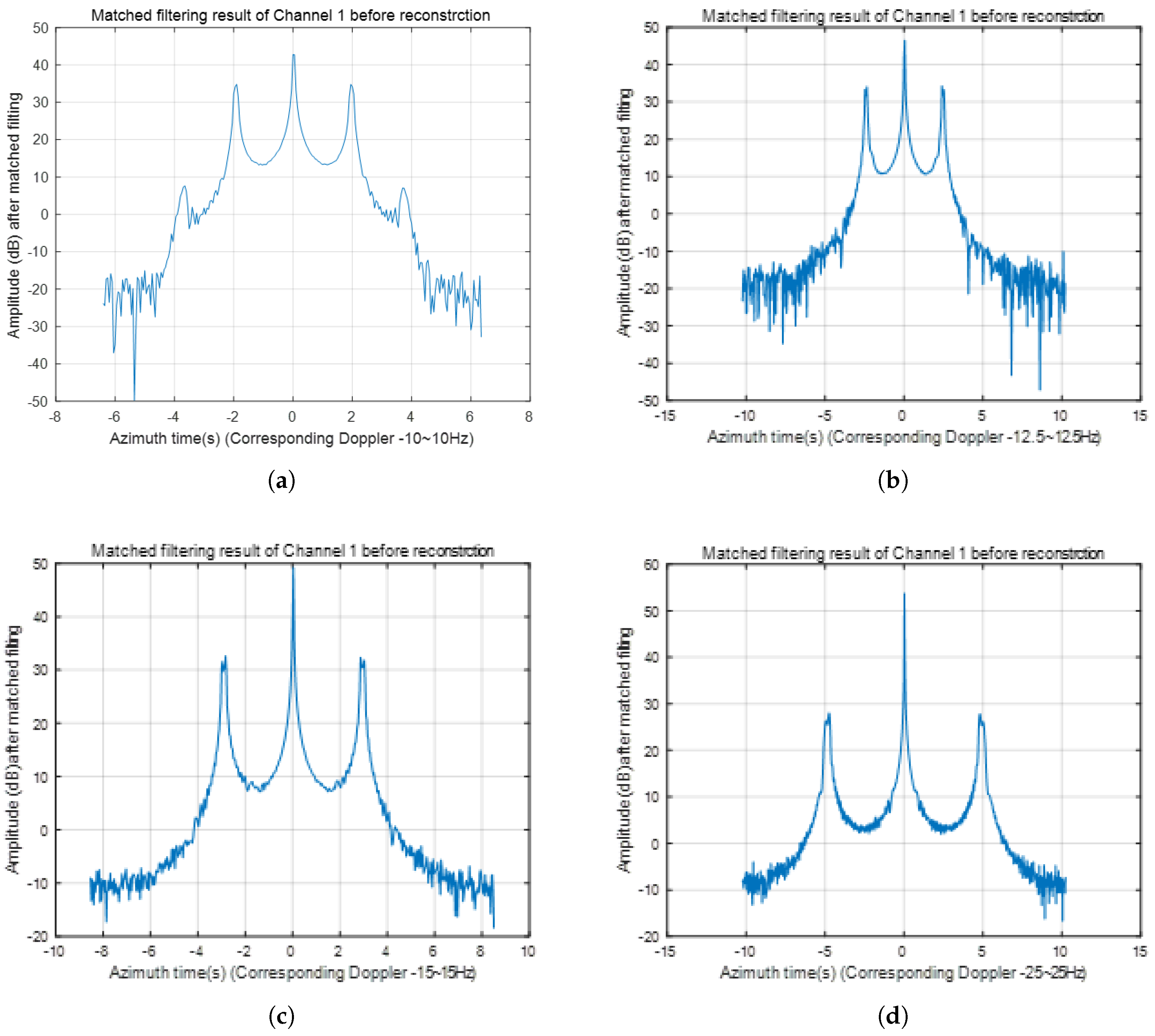
Matched filtering results of the five-channel SAR system’s Channel 0 before reconstruction with different PRF values: (a) Sampling at PRF = 20 Hz and the corresponding ambiguity index. (b) Sampling at PRF = 25 Hz and the corresponding ambiguity index. (c) Sampling at PRF = 30 Hz and the corresponding ambiguity index. (d) Sampling at PRF = 50 Hz and the corresponding ambiguity index.
Figure 3.
Matched filtering results of the five-channel SAR system’s Channel 0 before reconstruction with different PRF values: (a) Sampling at PRF = 20 Hz and the corresponding ambiguity index. (b) Sampling at PRF = 25 Hz and the corresponding ambiguity index. (c) Sampling at PRF = 30 Hz and the corresponding ambiguity index. (d) Sampling at PRF = 50 Hz and the corresponding ambiguity index.
4.1. Simulation Verification
A vehicle-borne simulation SAR scenario with five azimuth spatial channels is presented first. Table 2 lists the parameters of the simulation system. Assuming no range synchronization time or channel amplitude errors, the simulation parameters only set the channel phase errors. The echo data are sampled at PRF values of 20 Hz, 25 Hz, 30 Hz, and 50 Hz, respectively. We can observe that the ambiguity index varies with different PRF values. For example, when PRF = 15 or 20 Hz, the index i is -2, -1, 0, 1, 2; and when PRF = 30 or 50 Hz, the index i is -1, 0, 1, as shown in Figure 3. We then carry out the imaging process, which includes two-dimensional matched filtering and RCMC, for each channel at PRF = 50 Hz.
We then carry out the imaging process, which includes two-dimensional matched filtering and RCMC, for each channel at a fixed PRF. In this experiment, channel 0 is set as the reference channel. Furthermore, the channel errors are set as , , , , and , as listed in Table 3. Since the Doppler bandwidth of the echo signal is larger than the PRF setting, aliasing occurs. As a result, the point target cannot fully focus in the image, which reveals ghost targets in each channel’s final image, as depicted in Figure 4. However, it still displays the phases of the dominant peak in each sub-channel’s final image, and after calculating the difference between these peak phases, we find that the differences are nearly the same as the channel errors we set, as shown in Table 4. In addition, the PRF of the simulation is set to 17 Hz, so the equivalent PRF after reconstruction is , which is larger than the Doppler bandwidth of 80.333 Hz presented in Table 1.
The data summarized in Table 4 indicate that the phase error information among channels is carried by each channel and is reflected in the phase differences of the dominant peak point from the independent imaging before reconstruction. This constitutes the core principle of the method proposed in this article. Meanwhile, the simulation scenario here has a 0 Hz Doppler centroid, so the phase differences among channels represent the channel phase errors.
Alongside the phase error estimation, the steering matrix for each Doppler frequency band is accurately constructed to correspond to the specific ambiguity index. The phase errors among sub-channels cause a frequency shift in the reconstructed Doppler spectrum, as depicted in Figure 5a. This leads to filter mismatching and the appearance of false targets in pairs during subsequent reconstruction processing. By utilizing the estimated phase errors in the reconstruction process, we can effectively weight the echo data from each channel and reconstruct the signal. Figure 5b shows the reconstructed Doppler band after correcting for the channel errors. Then, after performing Doppler-matched filtering using a conventional method, we observe that the characteristic point of the reconstructed signal is well-focused. Figure 5c and Figure 5d compare azimuth reconstruction, where one scenario demonstrates no estimation errors and the other shows results using the calibration errors, validating the proposed algorithm. The above image results not only highlight the importance of channel error estimation in the signal reconstruction of multi-channel SAR systems but also demonstrate the feasibility and accuracy of the proposed algorithm.
Then, the channel errors are obtained using the cross-correlation algorithm in the spatial time-domain and the subspace algorithm in the Doppler frequency domain, and the reconstruction of the echo signal is completed. These results are compared with those obtained using the algorithm proposed in this article. Specific parameters are set to evaluate the performance differences between the proposed algorithm and the other two classical algorithms. The PRF is set to 17 Hz, resulting in an equivalent PRF of 85 Hz after reconstruction, which is larger than the Doppler bandwidth. The SNR is set to 30 dB, 20 dB, 10 dB, and 0 dB to evaluate the performance fluctuations of different methods at varying SNR levels. The results of the channel error estimation are shown in Table 5.
Compared to the cross-correlation algorithm, the proposed method conveniently estimates channel errors using ready-made imaging tools and software. Compared to the subspace algorithm, the proposed method’s estimation performance does not depend on the SNR value. Additionally, it achieves results with lower computational cost, particularly at high SNR levels, where the subspace method can calculate accurately. This comparison demonstrates the robustness of the proposed method. Additionally, when the SNR is 20 dB, phase errors are obtained using three algorithms, and the signals are reconstructed, as shown in Figure 6. The reconstructed signal, utilizing the channel errors obtained by the proposed method, exhibits good focusing performance in the azimuth direction. Observing the data in Table 5 reveals that, overall, the subspace algorithm is the most accurate, while the accuracy of the proposed method and the cross-correlation algorithm is relatively low. However, as shown in Figure 6, the reconstruction performance of the proposed method, despite its relatively poor estimation accuracy, is not significantly different from that of the subspace algorithm. Nevertheless, given the high computational cost of the subspace algorithm, the proposed method offers a significantly lower computational load.
4.2. Airborne Data Verification
In this subsection, an airborne verification is conducted using a multi-channel SAR system. The generated data is used to estimate channel errors using the method proposed in this article, followed by reconstruction and 2D matched filtering to produce the final image. In multi-channel mode, the phased-array antenna operates with one digital channel transmitting signals in the azimuth direction, while three digital channels receive the echo signals, forming an azimuth-oriented 3-channel SAR system. Figure 7 shows the geometric model of the antenna. The antenna consists of four columns arranged along the azimuth direction. In this configuration, the signal is transmitted by the second column on the right and received by the first, second, and third columns on the right. The equal azimuthal size of the transmitting and receiving antennas ensures the same azimuth-oriented 3dB beamwidth. The multi-channel SAR system operates in the X band, with one TR unit arranged per column along the azimuth direction. Each column antenna has an azimuth length of 0.264 m and a beamwidth of approximately . Each column antenna contains 24 TR units arranged along the range direction, with a length of 1.008 m and a beamwidth of approximately 1.. Thus, the output power of each column’s TR units is approximately . Before the flight test, the phases of the TR’s transmitting and receiving units were adjusted while the RF cables were equipped. The antenna pattern was also tested. Additionally, apart from the transceiver channels, the phased-array antenna includes three calibration channels, as shown in Figure 7.
During flight verification, the SAR system is installed on a manned aircraft, with the antenna mounted on the aircraft’s side wall for imaging. The installation of the antenna on the aircraft is shown in Figure 8. During multi-channel SAR mode imaging, the aircraft flies at an altitude of 4000 m, producing images with a side-look angle of . The aircraft flies at a speed of 61 m/s, with a system Doppler bandwidth of 463 Hz. The multi-channel mode of the SAR system operates with a PRF of 200 Hz, corresponding to an azimuth sampling rate of 200 Hz. In conventional single-channel imaging, the azimuth sampling rate does not satisfy Nyquist’s criterion, leading to aliasing or azimuth ambiguity. Table 6 summarizes the system and imaging scene parameters.
The flight-testing airspace was located in Liangping District, Chongqing. After analyzing the optical image of the imaging region on Google Earth, a more suitable area for imaging was identified, as shown in Figure 9. The imaging region contains many prominent features, such as airports, farmland, rivers, roads, and artificial buildings, making it well-suited for imaging observation.
Imaging data were processed based on the parameters listed in Table 6. First, the three channels were imaged separately, and the image of channel 1 is shown in Figure 10a. Due to the insufficient sampling rate, imaging of separate channel data before reconstruction leads to ambiguity. However, the salient objects in the imaging scene can still be identified. Sub-channel 1 is designated as the reference channel, while sub-channel 2 and sub-channel 3 require calibration. The images from each of the three sub-channels are divided into sub-images along the azimuth and range directions, as shown in Figure 10b. Characteristic clusters are then identified in the 16 sub-images. As mentioned above, a characteristic cluster refers to a well-focused cluster of points with high amplitude, surrounded by points with especially low values. A well-focused characteristic cluster is usually considered as a single point but appears as a set of multiple points due to ambiguity. The maximum amplitude point in a characteristic cluster is referred to as the characteristic point. The characteristic clusters in the 16 sub-images are identified and displayed in a single-channel image, as shown in Figure 10c. The pixel positions of the characteristic points in each cluster from the three sub-channel images are accurately obtained and listed in Table 7. It was found that the pixels with the largest amplitude values in each characteristic cluster have nearly identical positions in the images of the three sub-channels.
The positions of the characteristic points across the three channels are nearly overlapping, confirming the accuracy of the proposed method’s initial assumption. Meanwhile, the lagging-leading consistency of the range synchronization time among the sub-channels is reflected in the alignment of characteristic points along the range positions. Using the characteristic point as the center, interpolation is performed across the three channels in the range direction to obtain refined sampling errors. The final synchronization errors are calculated by weighted averaging of the errors derived from multiple characteristic points.
The amplitude and phase values of the characteristic points in the characteristic clusters of each sub-image across the three channels are obtained, and the channel phase errors between channels 2, 3, and 1 are calculated. It was found that the phase errors of the characteristic points in each cluster across all channels are generally within a relatively consistent range. Additionally, it was observed that when no certified characteristic clusters were present, or the maximum amplitude point was smaller, the error accuracy could be poor due to noise, which can be mitigated using the 3 method to ensure accurate error estimation. The characteristic points are then sorted according to amplitude, with the highest coefficients assigned to the errors of the four largest characteristic points, and lower coefficients assigned to the others. Similarly, if any phase errors of the four largest characteristic points do not meet the 3 standard within a relatively small numerical range, their coefficient assignment is reduced to a lower level. By calculating the weighted average of multiple phase errors, the phase error between channel 2 and channel 1 is found to be 150., and the phase error between channel 3 and channel 1 is 139.. The recorded and calculated data are shown in Table 8.
By examining the distribution of the signal centroid in the Range-Doppler domain, we find that the Doppler centroid is -205.44 Hz. The fixed channel difference between channel 2 and the reference channel is calculated as , and between channel 3 and the reference channel as . Finally, the channel errors are calculated as and . Additionally, the weighted amplitude and range synchronization time delays are obtained using the method proposed in this article. The final spectrum is then reconstructed, and the reconstructed data are processed using traditional SAR methods, yielding the final image shown in Figure 11. A detailed image using the proposed method is displayed in Figure 12.
5. Discussion
In Section 4, the proposed method is validated through simulations of the five-channel SAR system and actual airborne three-channel SAR data.
As shown in Figure 3, adjusting the ambiguity index and the steering matrix according to the PRF sampling rate and Doppler spectrum is a crucial step. The data in Table 3, Table 4, and Figure 3 indicate that Figure 4 implicitly shows that phase error information among channels is carried by each channel and is reflected in the phase differences of the dominant peak point from the independent imaging before reconstruction. This is the core principle of the method proposed in this paper. Through simulation, Figure 5 illustrates the importance of phase error calibration for signal reconstruction when phase errors exist among the five channels. As shown in Figure 3, it is crucial to adjust the ambiguity index and the steering matrix according to the Doppler spectrum before estimating the channel errors. Figure 3 and Table 2 demonstrate the linearity of the systems presented in Section 3. Figure 6 and Figure 7, and Table 4 show that the proposed method achieves higher accuracy than traditional methods, such as the time-domain correlation method and the orthogonal method, particularly at low SNR levels. In general, compared to traditional methods, the proposed method does not require iteration or the complex decomposition of the covariance matrix’s eigenvalues, which significantly reduces the computational load. Table 5 compares the channel error estimation results between the proposed algorithm and two classical algorithms under different SNR levels. Figure 6 displays the final signal reconstruction results of three phase estimation methods, as shown in Table 5, when the SNR is 20 dB.
In the airborne SAR data verification, Figure 7 and Figure 8 present the multi-channel antenna SAR system and the carrier environment. Table 6 and Figure 9 provide the flight imaging scenarios and imaging parameters. Figure 10 presents the results of the separate channel imaging and the characteristic clusters in the 16 sub-images. Table lists the detailed positions of each characteristic point across the three channels, from which the range synchronization time errors among channels can be estimated through interpolation. Table 8 lists the amplitudes and phases of the 16 characteristic points. Based on the amplitude size order, the weighted average values of the amplitudes and phases are calculated to determine the phase differences and amplitude errors among channels. Figure 11 and Figure 12 show the final imaging results after reconstruction using the error estimations produced by the proposed algorithm.
From the experimental results, compared to traditional methods such as the time-domain correlation method and the orthogonal method, it can be seen that the proposed method does not require iteration or solving the complex problem of eigenvalue decomposition of the covariance matrix. The accuracy of the proposed method is satisfactory. Moreover, the estimation process can be carried out using ready-made imaging tools and software, which makes it more convenient.
6. Conclusions
This article proposes a novel channel error estimation algorithm for the azimuth multi-channel SAR system. The formula expression in the two-dimensional time domain after single-channel processing is derived, assuming the azimuth sampling rate is insufficient. The error estimation method is then proposed using the characteristic point information across multiple channels. Finally, simulation trials and actual data are used to verify the method. In this algorithm, separate channel imaging is first performed under insufficient azimuth sampling rate. The image is then divided into a specified number of sub-images along the azimuth and range directions, where the characteristic clusters and points meeting the specified requirements are searched for. The channel errors are then estimated by statistically processing the parameters of the characteristic points. Simulation trials and actual data processing show that the proposed method can conveniently estimate channel errors using ready-made imaging tools and software. AI methods could even be employed to search for characteristic clusters and points, which warrants further investigation.
Author Contributions
All authors made significant contributions to the preparation of this manuscript. J.F. (Jing Feng) and L.C. (Longyong Chen) contributed to the methodology; J.Y. (Junhua Yang) supported data curation; X.Y. (Yihao Xu) assisted with software implementation. R.T. (Ran Tao) and H.H. (Hao Huan) supervised the research and reviewed the manuscript; W.Y. wrote the paper. All authors have read and approved the final version of the manuscript.
Funding
This research received no external funding.
Institutional Review Board Statement
Not applicable.
Informed Consent Statement
Not applicable.
Data Availability Statement
No new data were created or analyzed in this study. Data sharing is not applicable to this article.
Acknowledgments
The authors would like to acknowledge the support of the Jilin-1 MS-01A mission, particularly Tianjin Yunyao Aerospace Technology Co., Ltd. and Changguang Satellite Technology Co., Ltd., for providing the data. We also thank the anonymous reviewers and members of the editorial team for their insightful comments and valuable suggestions.
Conflicts of Interest
The authors declare no conflicts of interest.
Abbreviations
The following abbreviations are used in this manuscript:
| SAR | Synthetic Aperture Radar |
| HRWS | High Resolution Wide Swath |
| LFM | Linear Frequency Modulation |
| PRF | Pulse Repetition Frequency |
| PRT | Pulse Repetition Time |
| RCMC | Range Cell Migration Correction |
| SCCC | Spatial Cross Correlation Coefficient |
| SSP | Signal Subspace |
| OSM | Orthogonal Subspace Method |
| MVDR | Minimum Variance Distortionless Response |
| SNR | Signal Noise Ratio |
| LML-WME | Local Maximum-Likelihood-Weighted Minimum Entropy |
| WBPA | Weighted Back Projection Algorithm |
| GDM | Gradient Descent Method |
| LLN | Least L1-Norm |
References
- Aguttes, J.P. The SAR train concept: Required antenna area distributed over N smaller satellites, increase of performance by N. IEEE Geosci Proc. IGARSS, Toulouse, Fr. 2004, 1, 142–149. [Google Scholar]
- Goodman, N.A.; Lin, S.C.; Rajakrishna, D.; Stiles, J.M. Processing of multiple-receiver spaceborne arrays for wide-area SAR. IEEE Trans. Geosci. Remote Sens. 2002, 40, 841–852. [Google Scholar] [CrossRef]
- Krieger, G.; Fiedler, H.; Houman, D.; Moreira, A. Analysis of system concepts for bi- and multi-static SAR missions. in Proc. IGARSS, Toulouse, France, 2003, vol. 2, pp. 770–772.
- Li, Z.F.; Wang, H.Y.; Su, T.; Bao, Z. Generation of wide-swath and high-resolution SAR images from multichannel small spaceborne SAR systems. IEEE Geosci. Remote Sens. Lett. 2005, 2, 82–86. [Google Scholar] [CrossRef]
- Schindler, J.K.; Steyskal, H.; Franchi, P. Pattern synthesis for moving target detection with TechSat21—A distributed space-based radar system. in Proc. Radar, Edinburgh, U.K., 2002, pp. 375–379.
- Curlander, J.C.; McDonough, R.N. “Synthetic Aperture Radar: Systems and Signal Processing” New York, NY, USA: Hoboken, NJ, USA: Wiley, 1991.
- Cumming, I.G.; Wong, F.H. Digital Processing of Synthetic Aperture Radar Data: Algorithms and Implementation. Boston, MA, USA: Artech House, 2005.
- Huber, S.; de Almeida, F.Q.; Villano, M.; Younis, M.; Krieger, G.; Moreira, A. Tandem-L: A technical perspective on future spaceborne SAR sensors for Earth observation. IEEE Trans. Geosci. Remote Sens. 2018, 56, 4792–4807. [Google Scholar] [CrossRef]
- Feng, J.; Gao, C.; Zhang, Y.; Wang, R. Phase mismatch calibration of the multichannel SAR based on azimuth cross correlation. IEEE Geosci. Remote Sens. Lett. 2013, 10, 903–907. [Google Scholar] [CrossRef]
- Liu, Y.; Li, Z.; Wang, Z.; Bao, Z. On the baseband Doppler centroid estimation for multichannel HRWS SAR imaging. IEEE Geosci. Remote Sens. Lett. 2014, 11, 2050–2054. [Google Scholar]
- Li, Z.F.; Wang, H.Y.; Bao, Z.; Liao, G.S. Performance improvement for constellation SAR using signal processing techniques. IEEE Trans. Aerosp. Electron. Syst. 2006, 42, 436–452. [Google Scholar]
- Liu, A.F.; Liao, G.S.; Ma, L.; Xu, Q. An array error estimation method for constellation SAR systems. IEEE Geosci. Remote Sens. Lett. 2010, 7, 731–735. [Google Scholar] [CrossRef]
- Yang, T.; Li, Z.; Liu, Y.; Bao, Z. Channel error estimation methods for multichannel SAR systems in azimuth. IEEE Geosci. Remote Sens. Lett. 2013, 10, 548–552. [Google Scholar] [CrossRef]
- Guo, X.; Gao, Y.; Wang, K.; Liu, X. Improved channel error calibration algorithm for azimuth multichannel SAR systems. IEEE Geosci. Remote Sens. Lett. 2016, 13, 1022–1026. [Google Scholar] [CrossRef]
- Zhang, L.; Gao, Y.; Liu, X. Robust channel phase error calibration algorithm for multichannel high-resolution and wide-swath SAR imaging. IEEE Geosci. Remote Sens. Lett. 2017, 14, 649–653. [Google Scholar] [CrossRef]
- Hawkes, M.; Nehorai, A.; Stoica, P. Performance breakdown of subspace-based methods: Prediction and cure. in Proc. IEEE Int. Conf. Acoust. Speech Signal Process., May 2001, pp. 4005–4008.
- Khabbazibasmenj, A.; Vorobyov, S.A.; Hassanien, A. Robust adaptive beamforming based on steering vector estimation with as little as possible prior information. IEEE Trans. Signal Process. 2012, 60, 2974–2987. [Google Scholar] [CrossRef]
- Gu, Y.; Leshem, A. Robust adaptive beamforming based on interference covariance matrix reconstruction and steering vector estimation. IEEE Trans. Signal Process. 2012, 60, 3881–3885. [Google Scholar]
- Huang, H.; et al. A novel channel errors calibration algorithm for multichannel high-resolution and wide-swath SAR imaging. IEEE Trans. Geosci. Remote Sens. 2022, 60, 1–19. [Google Scholar] [CrossRef]
- Gao, C.-G.; Deng, Y.-K.; Feng, J. Theoretical analysis on the mismatch influence of displaced phase center multiple-beam SAR systems. J. Electron. Inf. Technol. 2011, 33, 1828–1832. [Google Scholar] [CrossRef]
- Gebert, N.; Krieger, G.; Moreira, A. Digital beamforming on receive techniques and optimization strategies for high-resolution wide-swath SAR imaging. IEEE Trans. Aerosp. Electron. Syst. 2009, 45, 564–592. [Google Scholar] [CrossRef]
- de Almeida, F.Q.; Younis, M.; Krieger, G.; Moreira, A. An analytical error model for spaceborne SAR multichannel azimuth reconstruction. in Proc. Int. Conf. Radar Syst. (Radar), Oct. 2017, pp. 1–6.
- Xiao, F.; Ding, Z.; Li, Z.; Long, T. Channel error effect analysis for reconstruction algorithm in dual-channel SAR imaging. IEEE Geosci. Remote Sens. Lett. 2020, 17, 1563–1567. [Google Scholar] [CrossRef]
- Liang, D.; et al. A channel calibration method based on weighted backprojection algorithm for multichannel SAR imaging. IEEE Geosci. Remote Sens. Lett. 2019, 16, 1254–1258.85. [Google Scholar] [CrossRef]
- Sun, G.; Xiang, J.; Xing, M.; Yang, J.; Guo, L. A channel phase error correction method based on joint quality function of GF-3 SAR dual-channel images. Sensors 2018, 18, 3131. [Google Scholar] [CrossRef]
- Sun, G.; et al. A postmatched-filtering image-domain subspace method for channel mismatch estimation of multiple azimuth channels SAR. IEEE Trans. Geosci. Remote Sens. 2022, 60, 1–14. [Google Scholar] [CrossRef]
- Zhang, S.; Xing, M.; Xia, X.; Liu, Y.; Guo, R.; Bao, Z. A robust channel-calibration algorithm for multi-channel in azimuth HRWS SAR imaging based on local maximum-likelihood weighted minimum entropy. IEEE Trans. Image Process. 2013, 22, 5294–5305. [Google Scholar] [CrossRef]
- Cai, Y.; Deng, Y.; Zhang, H.; Wang, R.; Wu, Y.; Cheng, S. An Image-Domain Least L1-Norm Method for Channel Error Effect Analysis and Calibration of Azimuth Multi-Channel SAR. IEEE Geosci. Remote Sens.Lett. 2022, 10, 548–552. [Google Scholar]
- Jao, J.K.; Yegulalp, A. Multichannel Synthetic Aperture Radar Signatures and Imaging of a Moving Target. Inverse Problems 2013, 29, 054009. [Google Scholar] [CrossRef]
Figure 1.
Geometric diagram of a multichannel HRWS-SAR system and a static ground-based characteristic cluster.
Figure 1.
Geometric diagram of a multichannel HRWS-SAR system and a static ground-based characteristic cluster.
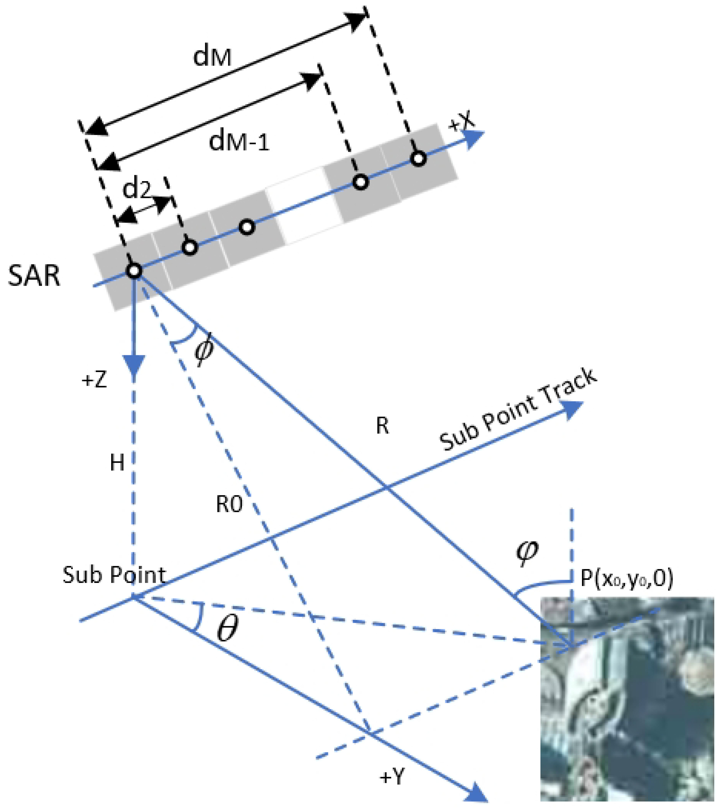
Figure 2.
Processing flowchart of the proposed method.
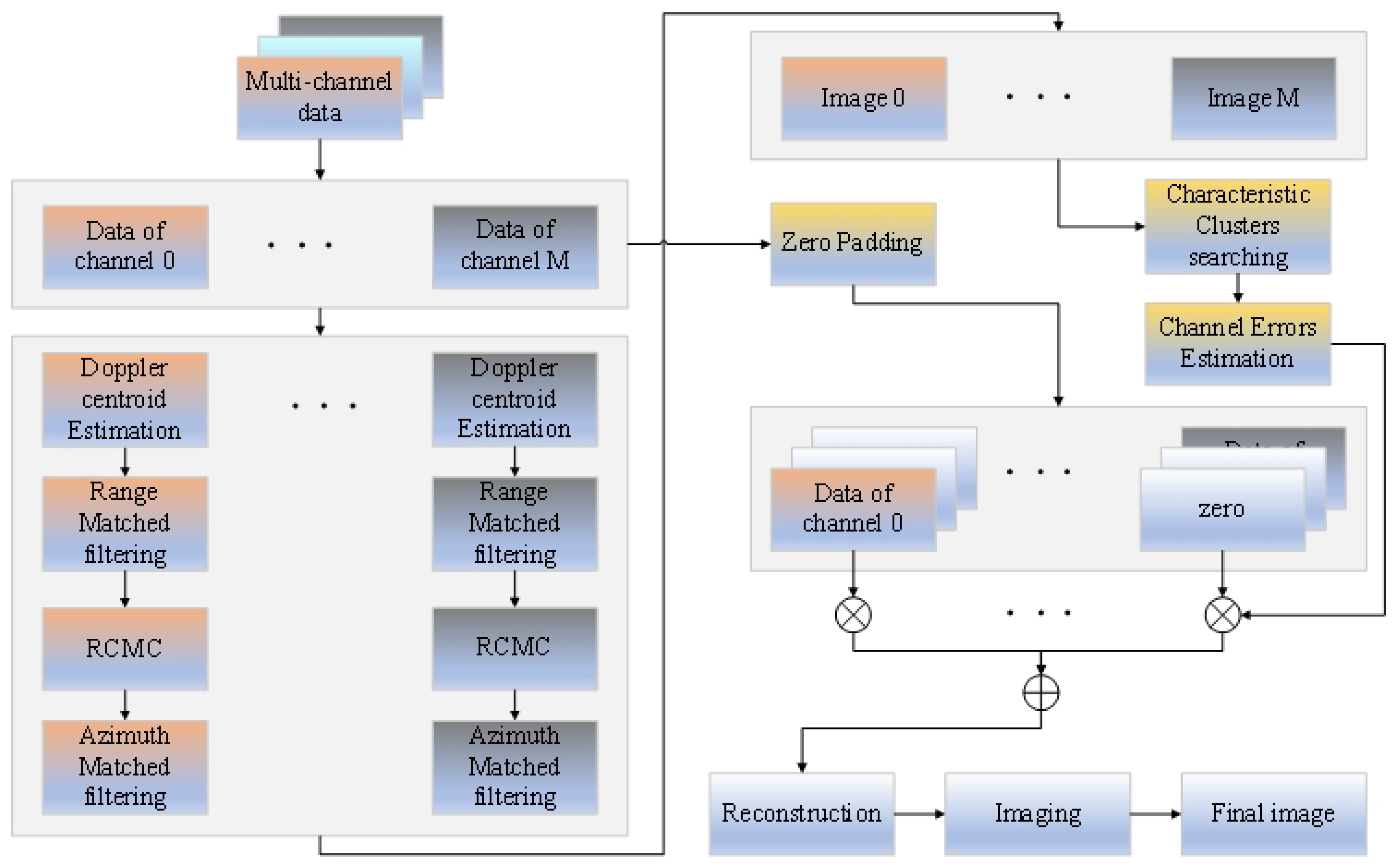
Figure 4.
Matched filtering results of the five-channel SAR system’s single channels before reconstruction: (a) Matched filtering result of channel 0. (b) Matched filtering result of channel 1. (c) Matched filtering result of channel 2. (d) Matched filtering result of channel 3. (e) Matched filtering result of channel 4.
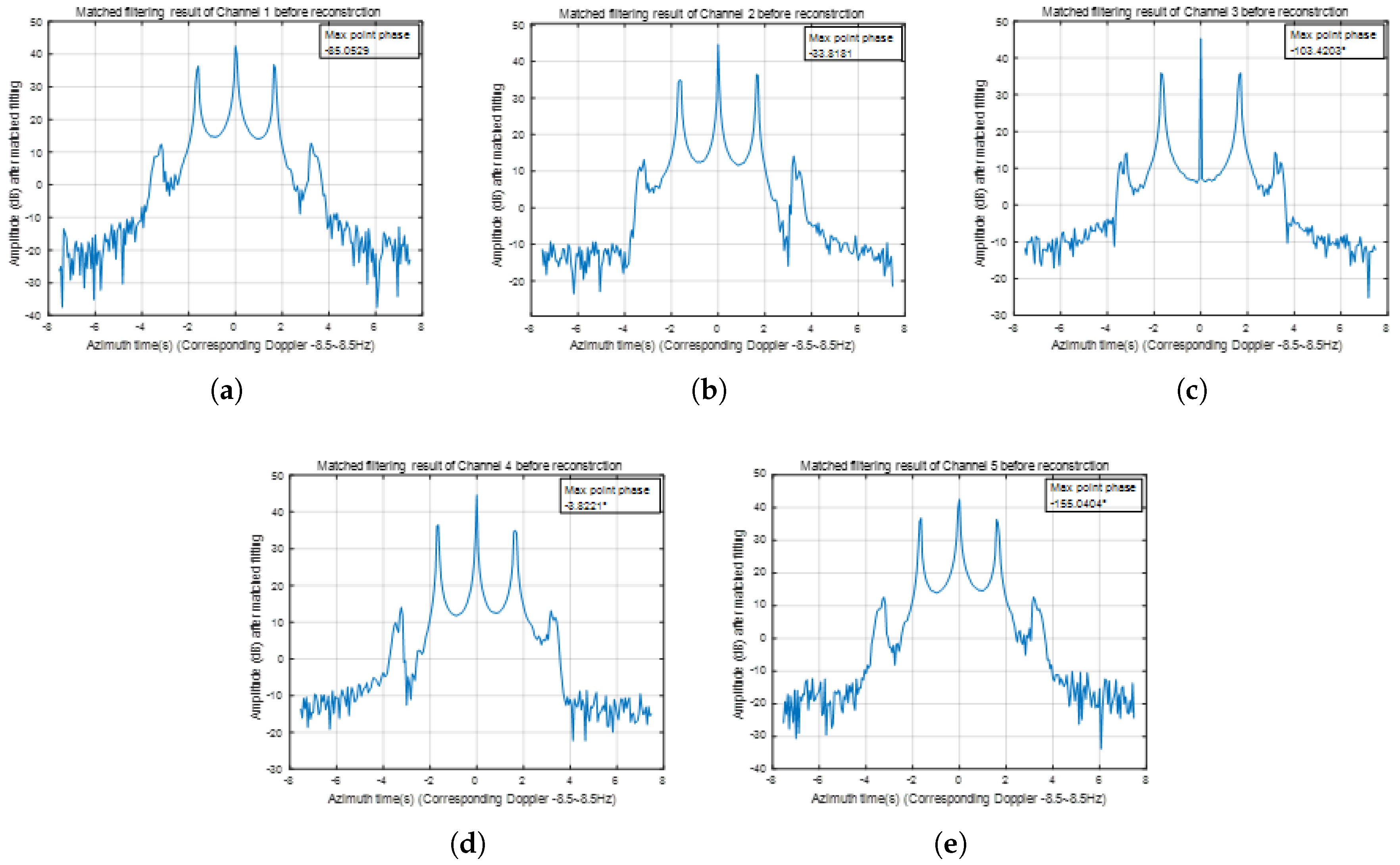
Figure 5.
Doppler spectrum and reconstructed echo results of a five-channel SAR system: (a) Doppler spectrum without channel error calibration. (b) Doppler spectrum using the proposed calibration method. (c) Reconstructed echo without channel error calibration. (d) Reconstructed echo using the proposed calibration method.
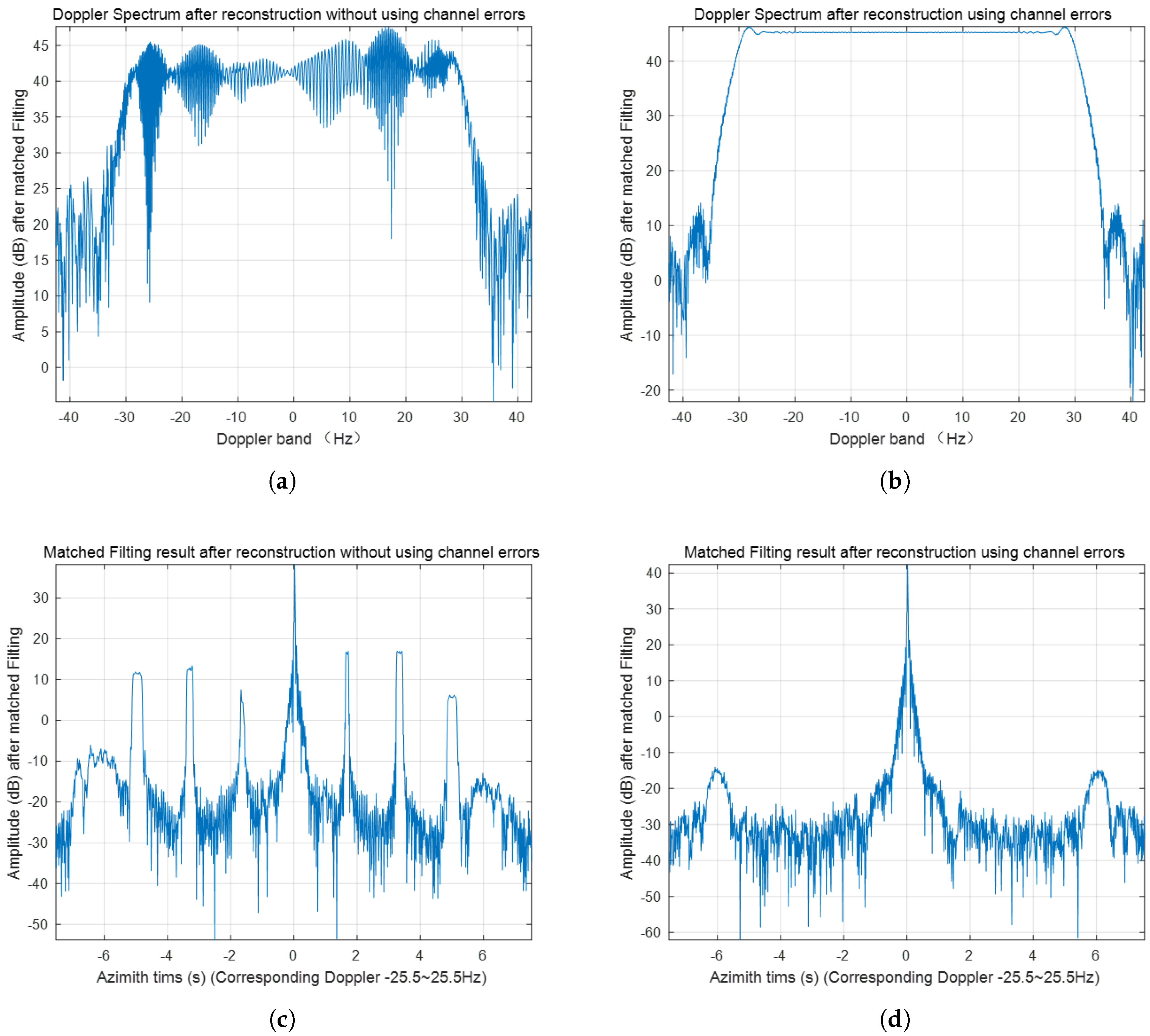
Figure 6.
Reconstruction performance using different channel error estimation methods: (a) Estimated results using the cross-correlation (TDCC) algorithm in the spatial time-domain. (b) Estimated results using the subspace (SS) algorithm in the Doppler frequency domain. (c) Estimated results using the proposed method.
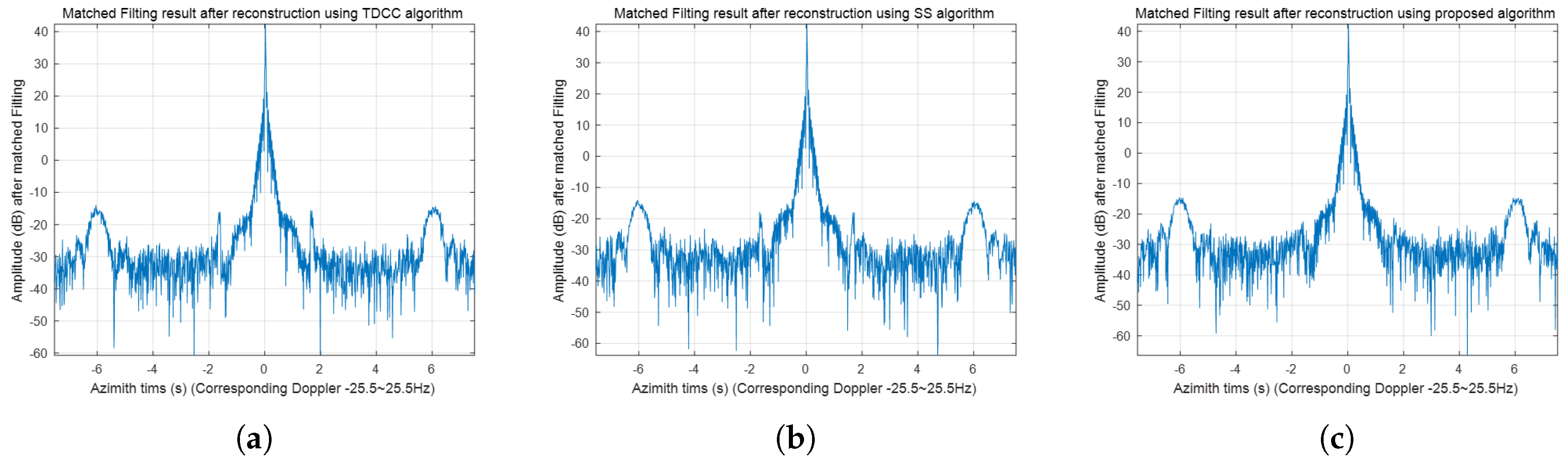
Figure 7.
Model of multi-channel phased-array antenna.
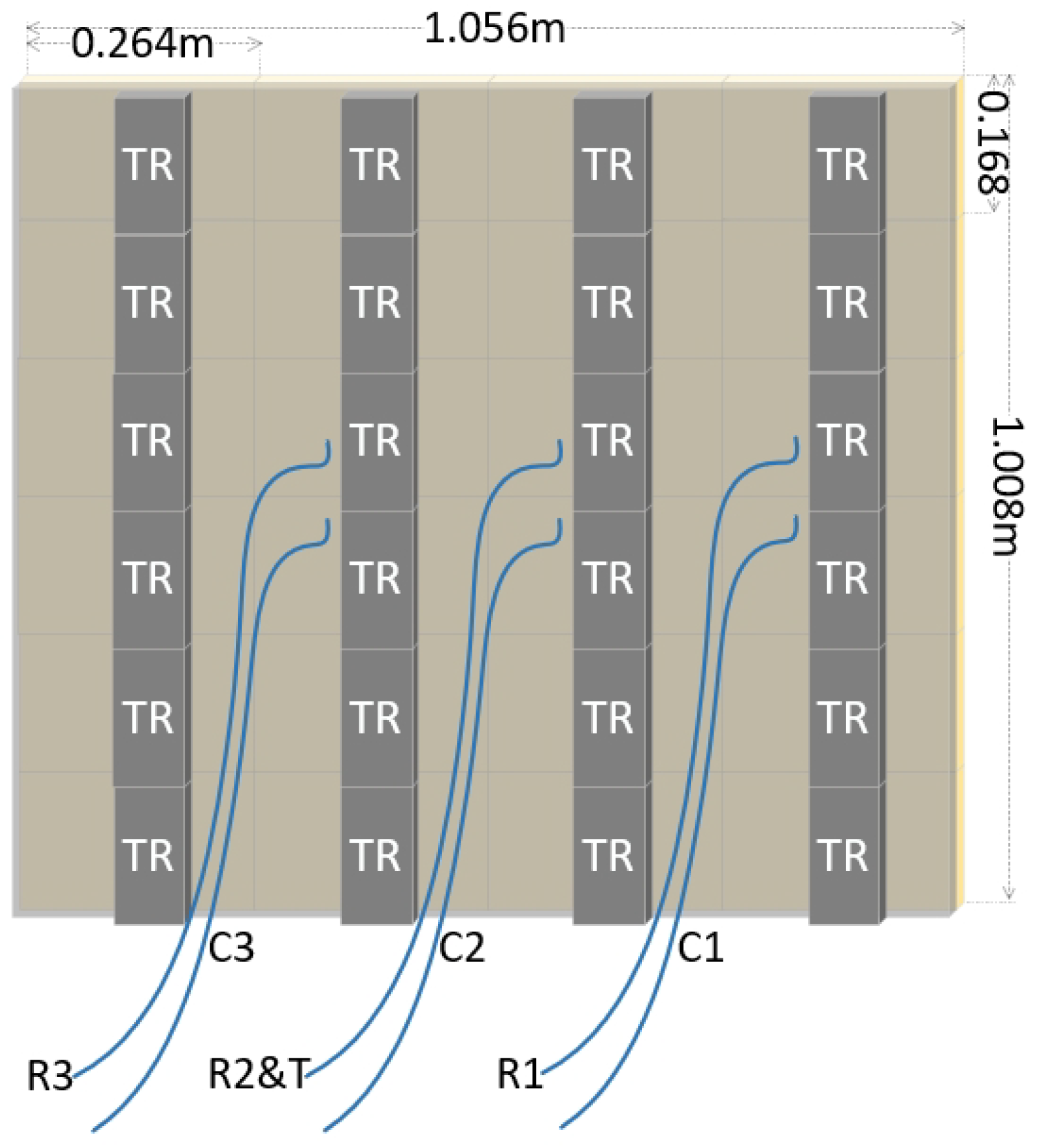
Figure 8.
Airplane mounted with multi-channel SAR system.
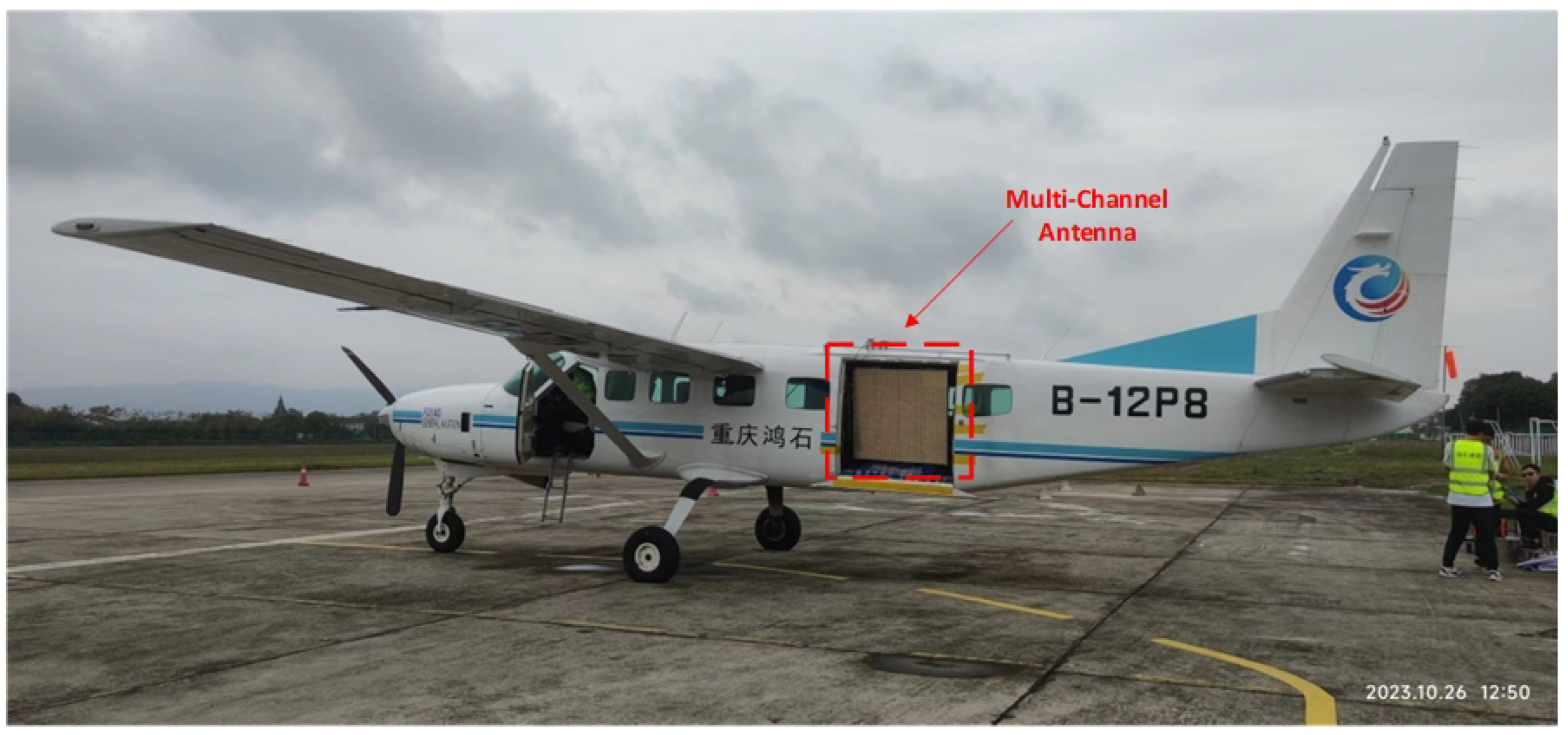
Figure 9.
Selected imaging scenes from Google Earth.
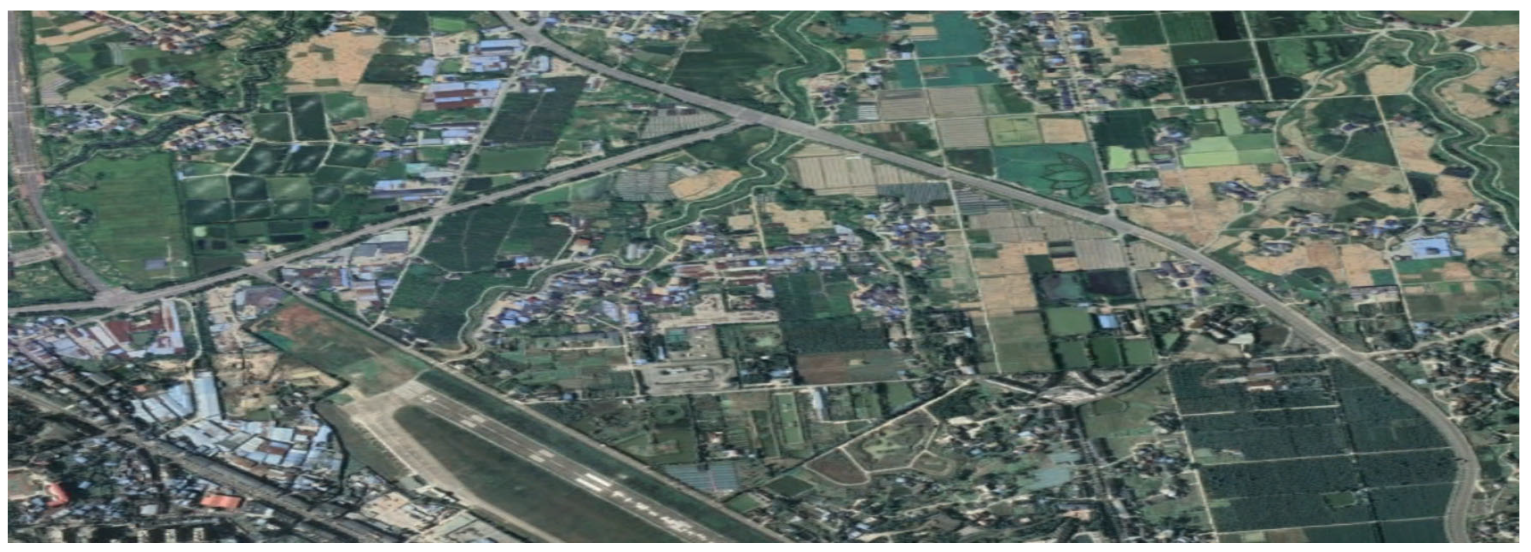
Figure 10.
Critical step results in processing. (a) Separately imaged results before construction of channel 1. (b) sub-images zoning along azimuth and range directions. (c) Characteristic clusters searching and marking in 16 sub-images.
Figure 10.
Critical step results in processing. (a) Separately imaged results before construction of channel 1. (b) sub-images zoning along azimuth and range directions. (c) Characteristic clusters searching and marking in 16 sub-images.
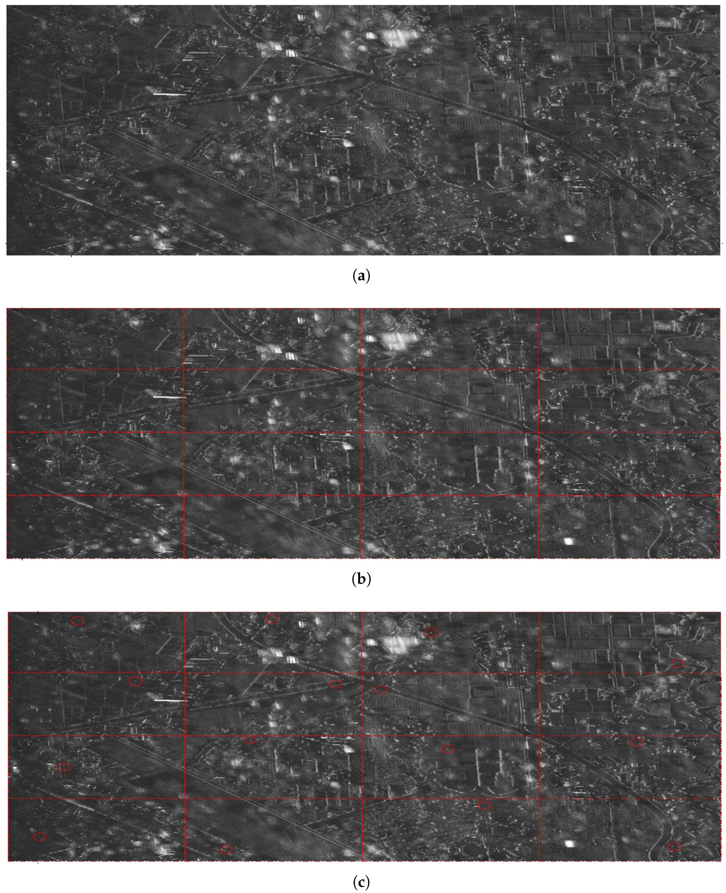
Figure 11.
Imaging results of the airborne SAR data using the proposed method.
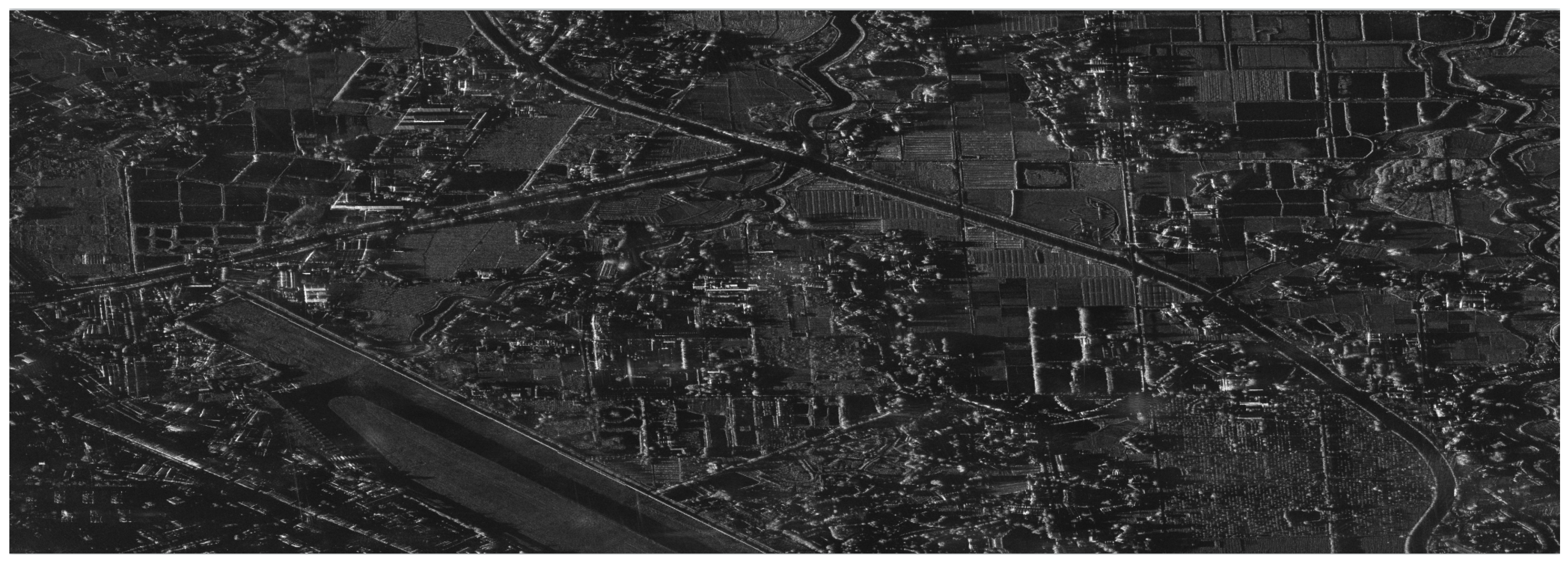
Figure 12.
Detailed image of the airborne SAR data using the proposed method.
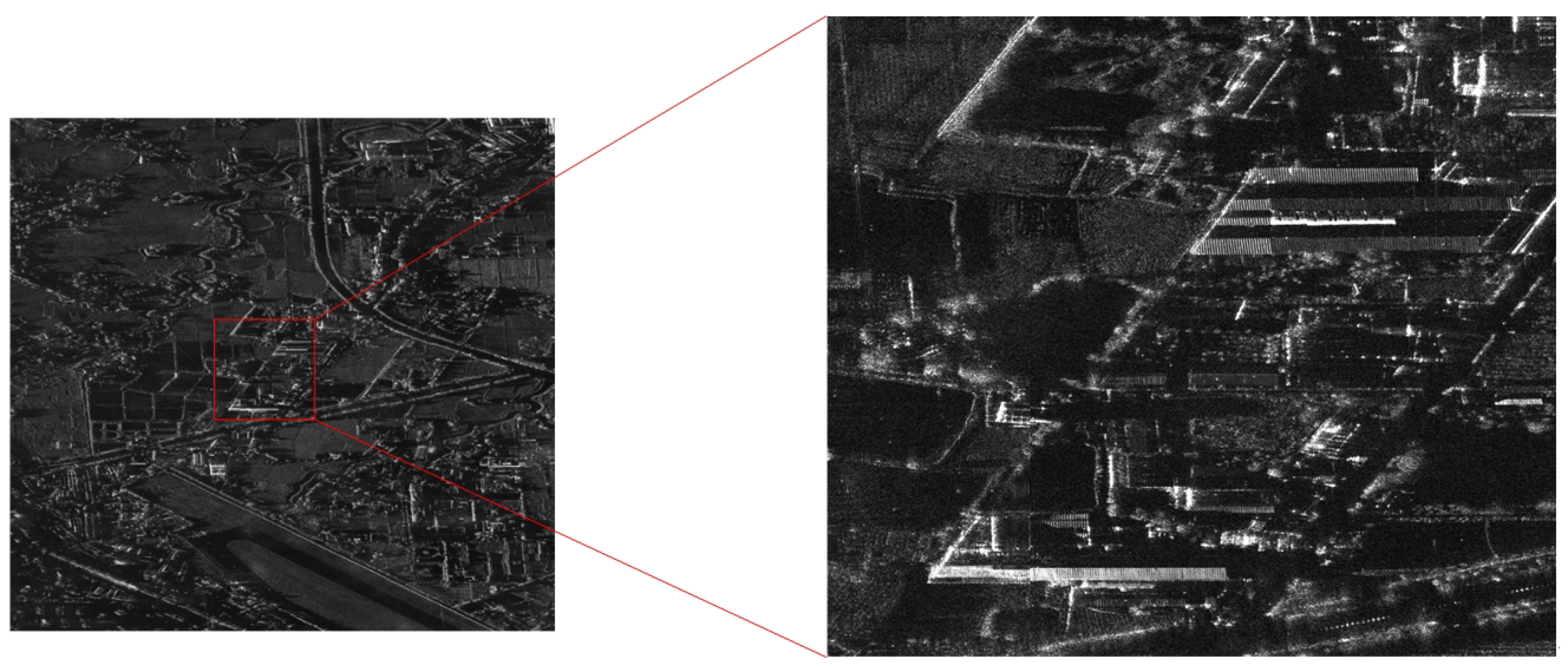
Table 1.
Weight coefficients of the ordered characteristic points according to the magnitude of the amplitude.
Table 1.
Weight coefficients of the ordered characteristic points according to the magnitude of the amplitude.
| Amp Order | ||||||||
| Coefficient | ||||||||
| Amp Order | ||||||||
| Coefficient | ||||||||
| Amp Order | ||||||||
| Coefficient | ||||||||
Table 3.
Channel Phase Errors’ Setting.
| Channel number | Phase Errors’ Setting |
|---|---|
| Channel 1 | |
| Channel 2 | |
| Channel 3 | |
| Channel 4 | |
| Channel 5 |
Table 4.
Max Point Phase in 5 Channels.
| Channel number | Phase of max point phase | Obtained phase error |
|---|---|---|
| Channel 1 | -85. | |
| Channel 2 | -33. | 51. |
| Channel 3 | -103. | -18. |
| Channel 4 | -3. | 81. |
| Channel 5 | -155. | -69. |
Table 5.
Estimation results of conventional methods and proposed method with different SNR.
| Channel Number | Real Phase Error | SNR | TDCC method | SS method | Proposed method |
|---|---|---|---|---|---|
| 0dB | |||||
| Channel 1 | 10dB | ||||
| 20dB | |||||
| 30dB | |||||
| 0dB | 51. | 51. | 51. | ||
| Channel 2 | 10dB | 52. | 50. | 51. | |
| 20dB | 51. | 50. | 51. | ||
| 30dB | 51. | 50. | 51. | ||
| 0dB | -16. | -17. | -18. | ||
| Channel 3 | 10dB | -17. | -19. | -18. | |
| 20dB | -17. | -19. | -18. | ||
| 30dB | -17. | -19. | -18. | ||
| 0dB | 80. | 81. | 81. | ||
| Channel 4 | 10dB | 81. | 81. | 81. | |
| 20dB | 81. | 80. | 81. | ||
| 30dB | 81. | 80. | 81. | ||
| 0dB | -73. | -70. | -69. | ||
| Channel 5 | 10dB | -69. | -69. | -70. | |
| 20dB | -70. | -70. | -69. | ||
| 30dB | -70. | -70. | -70. |
Table 6.
Airborne multi-channel SAR System Parameters.
| Parameter | Value |
|---|---|
| Wavelength | 0.03125m |
| Azimuth length of sub-channel antenna | 0.792 m |
| Range length of antenna | 1.008 m |
| Azimuth beamwidth of sub-channel antenna | |
| Range beamwidth of antenna | 1. |
| Instantaneous output power | 480 W |
| Channel number in azimuth | 3 |
| Flight height | 4000 m |
| SAR velocity | 61 m/s |
| Side-looking angle | |
| Doppler bandwidth | 463 Hz |
| Pulse repetition frequency | 200 Hz |
Table 7.
pixel positions of the characteristic points in all sub-images across the three channels.
| Sub-image Number | Channel Number | Azimuth Position | Range Position | Azimuth Position | Range Position | Azimuth Position | Range Position | Azimuth Position | Range Position |
|---|---|---|---|---|---|---|---|---|---|
| Channel 1 | 2516 | 4648 | 2543 | 7817 | 2728 | 10421 | 3551 | 14568 | |
| Sub-image 1-4 | Channel 2 | 2516 | 4646 | 2543 | 7815 | 2728 | 10420 | 3551 | 14567 |
| Channel 3 | 2516 | 4648 | 2542 | 7817 | 2727 | 10422 | 3550 | 14569 | |
| Channel 1 | 3949 | 5606 | 4010 | 8892 | 4149 | 9646 | 4142 | 13733 | |
| Sub-image 5-8 | Channel 2 | 3949 | 5604 | 4010 | 8891 | 4154 | 9646 | 4142 | 13732 |
| Channel 3 | 3949 | 5607 | 4009 | 8892 | 4152 | 9646 | 4142 | 13733 | |
| Channel 1 | 5999 | 3755 | 5288 | 7466 | 5533 | 10747 | 5380 | 13877 | |
| Sub-image 9-12 | Channel 2 | 5999 | 3754 | 5287 | 7464 | 5533 | 10745 | 5383 | 13876 |
| Channel 3 | 5998 | 3755 | 5287 | 7466 | 5532 | 10746 | 5383 | 13880 | |
| Channel 1 | 7586 | 4007 | 7903 | 7082 | 6851 | 11355 | 8080 | 14584 | |
| Sub-image 13-16 | Channel 2 | 7585 | 4005 | 7903 | 7081 | 6851 | 11353 | 8079 | 14581 |
| Channel 3 | 7585 | 4007 | 7902 | 7082 | 6850 | 11355 | 8078 | 14582 |
Table 8.
Recording, ordering and processing of the amplitude and phase of the characteristic points.
Table 8.
Recording, ordering and processing of the amplitude and phase of the characteristic points.
| Characteristic Point Number | C1 Amp | C1 Pha | C2 Amp | C2 Pha | C3 Amp | C3 Pha | Mean Amp | Amp Order | C2 Errors | C3 Errors |
|---|---|---|---|---|---|---|---|---|---|---|
| 1 | 679.60 | -136.94 | 625.08 | -4.14 | 658.84 | -43.68 | 654.51 | 10 | 132.80 | 93.26 |
| 2 | 517.21 | 88.14 | 404.95 | -140.61 | 541.78 | -118.01 | 487.98 | 13 | 131.25 | 153.85 |
| 3 | 991.99 | 35.89 | 1154.70 | 152.70 | 1110.50 | 128.50 | 1085.73 | 5 | 116.81 | 92.61 |
| 4 | 2610.70 | -96.62 | 2535.08 | 81.70 | 2823.50 | 40.32 | 2656.43 | 1 | 178.32 | 136.94 |
| 5 | 972.18 | 26.58 | 1019.20 | -171.20 | 930.32 | -169.90 | 973.90 | 6 | 166.22 | 163.52 |
| 6 | 1274.10 | -131.39 | 1194.10 | 21.60 | 1294.60 | 8.82 | 1254.27 | 4 | 152.99 | 140.21 |
| 7 | 592.19 | 132.07 | 630.38 | -119.90 | 588.91 | -108.03 | 603.83 | 12 | 108.03 | 119.90 |
| 8 | 662.16 | 170.29 | 699.24 | -9.84 | 541.20 | -18.72 | 634.20 | 11 | 179.87 | 170.99 |
| 9 | 882.95 | 11.55 | 708.28 | 168.26 | 794.56 | 142.76 | 795.26 | 9 | 156.71 | 131.21 |
| 10 | 832.25 | -178.55 | 925.88 | -12.67 | 816.25 | -47.21 | 858.13 | 8 | 165.88 | 131.34 |
| 11 | 226835 | -160.53 | 1943.30 | -24.86 | 2347.6 | -45.44 | 2186.47 | 2 | 135.67 | 115.09 |
| 12 | 336.15 | 70.00 | 474.88 | 130.60 | 342.04 | -46.01 | 384.36 | XXX | 60.60 | 243.99 |
| 13 | 990.86 | 105.32 | 851.95 | -59.38 | 903.45 | -107.22 | 915.42 | 7 | 195.30 | 147.46 |
| 14 | 1422.80 | 3.84 | 1497.30 | 152.17 | 1421.00 | 145.64 | 1449.03 | 3 | 148.33 | 141.80 |
| 15 | 255.23 | -48.04 | 232.44 | 109.57 | 321.58 | 98.18 | 269.75 | 15 | 157.61 | 146.22 |
| 16 | 460.88 | -33.33 | 393.69 | 167.9 | 462.81 | 162.19 | 439.13 | 14 | 201.23 | 195.52 |
Disclaimer/Publisher’s Note: The statements, opinions and data contained in all publications are solely those of the individual author(s) and contributor(s) and not of MDPI and/or the editor(s). MDPI and/or the editor(s) disclaim responsibility for any injury to people or property resulting from any ideas, methods, instructions or products referred to in the content. |
© 2025 by the authors. Licensee MDPI, Basel, Switzerland. This article is an open access article distributed under the terms and conditions of the Creative Commons Attribution (CC BY) license (http://creativecommons.org/licenses/by/4.0/).
Copyright: This open access article is published under a Creative Commons CC BY 4.0 license, which permit the free download, distribution, and reuse, provided that the author and preprint are cited in any reuse.


