
Submitted:
08 January 2025
Posted:
11 January 2025
You are already at the latest version
Abstract
This paper introduces a bi-level Kalman filter algorithm to estimate and predict traffic states required for real-time traffic signal control. Leveraging probe vehicle and upstream detector data, turning movement (TM) counts in the vicinity of signalized intersections are estimated at the upper level, while the upstream approach density and queue sizes are estimated at the lower level. The proposed approach was evaluated using drone-collected and simulated data at a four-legged signalized intersection in Orlando, Florida. The results of the bi-level approach were quantified relative to the baseline estimation without a Kalman filter. Results show that the Kalman filter is effective in enhancing traffic state estimates at various market penetration levels, where the filter both improves the estimation accuracy over the baseline case and provides reliable state predictions. At the upper level, the standard deviation (SD) in TM estimates improves by up to 50%, compared to the estimates provided by the sole use of probe vehicle headings. The proposed approach also provides predictions with a minimal SD of 92.8 veh/h at a 5% level of market penetration. At the lower level, the proposed queue size estimation method results in an enhancement to the queue size estimation of up to 32.8% compared to the estimates obtained from the baseline approach. In addition, the estimated traffic density is enhanced by up to 18.5%. The proposed bi-level approach demonstrates the capability of providing reliable turning movement predictions across varying levels of market penetration. This highlights the readiness of this approach for practical application in real-time traffic signal control systems.
Keywords:
Turning movement counts
; Kalman filters
; queue estimation
; connected vehicles
; traffic signal control
1. Introduction
Knowledge of turning movements (TMs) and queue sizes at signalized intersections is essential for numerous traffic applications, including conducting traffic analyses, traffic signal optimization, and evaluating the performance of the transportation system, especially for real-time applications. Specifically, predicting the traffic stream density and number of queued vehicles at signalized intersection approaches is critical for real-time adaptive traffic signal controller. However, accurate TM counts and queues are hard to obtain because they require exhaustive data collection efforts. Traditional data collection methods such as manual counts are still dominant; however, manual observation is labor-intensive and subject to human errors. The advancement of connected vehicle (CV) technologies provides the opportunity to enhance the data collection effort and provide more information about traffic states. Recently, probe data have been leveraged to obtain TMs as well as queue sizes at signalized intersections with high levels of accuracy [1]. However, solely relying on probe data for traffic state estimation has weaknesses, as this method becomes increasingly unreliable at lower levels of market penetration. As such, statistical recursive estimators, such as Kalman filters, are used to improve the estimation accuracy and provide future traffic state predictions.
To address this need, this study proposes a bi-level estimation and prediction approach for real-time TMs, upstream link density, and the number of queued vehicles per direction at signalized intersections. The proposed approach provides horizon predictions, on a real-time basis, leveraging upstream loop detectors and probe vehicle data. The proposed Kalman filtering algorithm is designed to estimate and predict the real-time number of turning vehicles in the upper level, with the prediction horizon adaptable depending on the application’s requirements, which can be as short as 1, 5, and 10 seconds. Thus, the estimated TMs are utilized in the lower level for queue size and density estimation, which is conducted for each TM. The proposed approach provides the essential information that facilitates the field implementation of advanced traffic signal optimization systems, such as the game-theoretic traffic signal controller proposed by [2], which requires real-time predictions of TMs and queue size for each lane group.
2. Literature Review
2.1. Estimation of Turning Movement Counts
Numerous efforts in the literature have approached the turning movement estimation problem at signalized intersections using loop detector data. As the approaching traffic flow counts are relatively easy to obtain using detectors or other stationary sensors, multiple methods have been proposed in the literature to infer TMs using approaching flows. The manual trial-and-error technique is one of the methods that requires obtaining inflow and outflow traffic at all the approaches of the intersection. This approach is considered tedious and difficult in terms of mathematical calculations and efficiency [3]. Some studies presented more robust techniques to estimate the most likely origin-destination matrix for intersections, which best replicates the observed approach counts, such as the work of Hauer et al. [4], which estimated the matrix using a likelihood maximization approach using Kruithof’s algorithm. This technique showed acceptable estimation accuracy; however, prior knowledge about actual TMs is critical to perform this approach. In addition, this method requires the deployment of detectors in all directions that carry traffic to and from the intersection. Van Aerde et al. [5] developed a tool for estimating an origin-destination (OD) demand matrix. The tool utilizes a maximum-likelihood-based numerical solution that does not require flow continuity at the network nodes. It is noted that the origin-destination problem is under-specified, where multiple solutions will provide a match to the counts. The maximum likelihood is used to select the most likely of these solutions. A seed matrix can also be used to bias the solution towards the seed matrix.
More recent studies presented other methods to estimate TMs, such as the work of Xu et al. [6], which developed an automatic TM identification system (ATMIS) that estimates TMs on a real-time basis. Another study by Zhang et al. [7], which estimated TMs using a non-linear programming approach using inflow and outflow counts. This approach shows high consistency compared to actual TMs. However, these methods still require outflow detectors to obtain acceptable estimates.
Chen et al. [8] also used a non-linear path flow-based algorithm to estimate TMs at a network level based on counts across the entire network. The study showed promising results in terms of estimation accuracy. However, the algorithm’s iterative process is considered difficult for real-time field applications in which TM estimations are required for short periods (e.g. 10-30 seconds).
Some studies used a genetic algorithm for TM estimations, such as the work of Jiao et al. [9], which estimated TMs in real time by minimizing the deviations between observed and estimated traffic counts. Ghanim et al. [10] used artificial neural networks (ANNs) for the estimation. Results of the developed ANN model showed that ANNs can be used to accurately estimate TMs. Mousavizadeh et al. [11] utilized probe vehicle data for turning rate estimation at large-scale urban networks using a Wavelet transform decomposition, using an estimation model that requires historic TM data. However, the training of machine learning models and the training of such estimation models based on hostoric data are considered computationally expensive and cannot be generalized beyond the context of the training data, such as the application to different characteristics of intersections, driving behavior, and demand patterns.
Some studies adopted a nonlinear least-square approach for the TM estimation problem such as the work of Lan et al. [12], which performed real-time TM estimation using partial counts on urban networks. The study employed a recursive nonlinear least-square approach using a partial set of detector counts. Similarly, Mirchandani et al. [13] presented a least-square minimization TM prediction algorithm implemented on a real-time basis. The algorithm is based on phase-to-phase counts that require the current turning proportions for prediction.
Finally, recent advancements in CV technologies have also been leveraged to estimate TMs, such as the work of Saldivar et al. [14], which used CV trajectory data to estimate TMs at signalized intersections. Entry and exit trajectory headings were used to detect the number of movement clusters using k-means clustering, which were assigned to a TM. A matching accuracy of up to 98% was achieved for over 1.1 million analyzed trajectories.
2.2. Queue Size Estimation from Probe Vehicles
The real-time queuing information at isolated intersections is essential information for the optimal control of traffic signals. The advancements in connected and automated vehicle technology allow the traffic signal controller to use probe vehicle data to make queue size estimates. There are vast literature on the topic of queue estimation, where it is mainly addressed in two primary estimation techniques: The input-output method and the shockwave theory. The input-output method estimates the number of vehicles within the queue, whereas the shockwave theory emphasizes the spatial extent of the queue. Furthermore, the queue estimation timeframe setting is categorized into a cycle-by-cycle queue length estimation and the real-time queue estimation [15].
Various methods of real-time queue estimation are reported in the literature such as the work of Comert et al. [16], which used a statistical method to estimate queue size in real-time from probe vehicle data. Based on the position of the probe vehicles in the queue, the queue size is estimated by a derived analytical expression. The study showed high estimation accuracy. However, it assumed that the marginal probability of queue size distribution is known, which is prior knowledge that is unavailable in many cases. Liu et al. [17] used a Markov model to estimate real-time queue size utilizing probe vehicle data. The average traffic flow rate, historical queue size data, and the stopping states for arriving probe vehicle data were used in the estimation procedure. The estimation scheme was tested for multiple market penetration levels of CVs. Results indicated high estimation accuracy and efficiency in handling the randomness in the system. One drawback is that the study relied on historical data, which might not be readily available. In addition, the categorization of queue size estimation by TM was also overlooked.
Another study by Zhao et al. [18] proposed a series of novel methods for real-time queue size estimation from probe vehicles. The proposed methods exploited the stopping positions of probe vehicles. The traffic volume and total queue size for each movement were obtained using the aggregated historical trajectory data. Study limitations include the inaccurate estimation of the market penetration rate using the last stopping position of probe vehicles. Shahrbabaki et al. [19] used a data fusion approach to estimate the second-by-second queue length. The proposed method showed notable estimation accuracy and efficiency.
Wei et al. [15] adopted an empirical Bayes method to estimate the cycle-based queue length, which showed significant estimation performance. Hao et al. [20] used a bayesian network model for estimating cycle-by cycle queue length. The study reported that 5% is the minimum market pentration rate for practical application of queue estimation using probe vehicles. However, the cycle-to cycle queue estimation methods are considered only applicable at conventional traffic signal contrllers where the phase lengths are known. Unlike other adaptive signals when the phase length are not known in advance.
2.3. Traffic State Estimation Using Kalman Filters
Kalman filters have been used for various applications in the domain of traffic management and control. For example, the Kalman filter has been used to estimate vehicle density and space-mean speeds at highways [21,22]. Antoniou et al. [23] used a nonlinear Kalman filter algorithm to calibrate online dynamic traffic assignment models; that algorithm showed a high level of accuracy as well as efficient computational performance. In addition, Emami et al. [24] used a Kalman filter algorithm for the short-term prediction of traffic flow in a CV environment.
Kalman filters have been used in the topic of traffic state estimation such as the work of Wang et al. [25], which used an extended Kalman filter algorithm to estimate the real-time traffic state. Bekiaris-Liberis et al. [26] also employed a Kalman filter to estimate the mixed traffic density at highways using the average speed of connected vehicles. Other studies utilized Kalman filter approaches to estimate TMs at signalized intersections. For example, Jiao et al. [27] developed a Bayesian approach, which is a combination of a back-propagation neural network model and a revised Kalman filter model. The algorithm employs historical data together with the present data to calibrate errors. While the reported results demonstrated high estimation accuracy, the algorithm’s reliance on historical data poses an applicability challenge due to its limited availability in many cases, despite the computational complexity involved. Another study by Zhang et al. [28] used a Kalman filter technique based on an extended cell transmission model (ECTM) to estimate TMs for adaptive traffic signal control systems. Results showed that the technique provided reliable traffic state estimates. Enjedani et al. [29] developed a Kalman filter TM estimator based on probe vehicle data, where probe data were considered representative of the total traffic flow for low market penetration levels. The method showed an improved TM estimation accuracy. However, the method also relies on historical data and is not applicable for short intervals of TM estimation; thus, it is not applicable for real-time applications of traffic signal optimization systems. Hu et al. [30] used an Extended Kalman filtering (EKF) approach for queue estimation at signalized intersection. The study used a machine learning model to construct the the shockwave queue propagation model. Then, the measured queue information is integrated in the EKF to derive real-time queue estimates.
2.4. Research Gap and Study Contribution
The use of a Kalman filtering approach has been extensively used in the literature for the purpose of traffic state, turning movement, density, and queue estimation. Most of the efforts in the literature reported traffic state estimation methods without categorizing the state estimates by turning movement, which is essential for some adaptive traffic signal controllers. In addition, the majority of the traffic state estimation methods are performed on highways rather than intersection approaches. The literature also reported the use of historic traffic data within Kalman filters to account for the estimation errors, which is unavailable in most cases and nonstationary. Furthermore, the use of machine learning with Kalman filtering can be limited by the availability of training data and cannot be extended beyond the scope of the historic data.
As such, this study contributes to the existing body of knowledge by proposing a bi-level Kalman filtering approach for traffic state estimation and prediction in the vicinity of traffic signals. The proposed approach bridges the research gap in the literature in the following ways:
- The proposed system is considered practical and computationally efficient for advanced real-time traffic signal controllers.
- The real-time traffic state estimates provided by the proposed system are categorized by turning movement, which is required for some adaptive traffic signal control applications.
- The proposed system does not require historical traffic information to calibrate the error covariance matrices in the Kalman filter, making it more practical compared to the cases where historical data are required to train machine learning models.
- The proposed system provides real-time traffic state estimation and predictions within variable short-term horizons to suite the requirements of some adaptive traffic signal controllers.
- The integration of real-time TM, density, and queue size estimation facilitates the system application in advanced traffic signal control systems that require real-time information on TM counts and queue size per movement.
3. Design of Kalman Filter
3.1. System Overview
A Kalman filter is an efficient recursive minimum variance estimator that follows a prediction-correction scheme. The Kalman filter integrates the recent previous state estimate with the current state observation to perform state estimation and future state projections. This algorithm was first developed by Kalman in 1960 [31]. The filter uses previous state estimates, new state observations, and projections of previous states to generate refined estimates of the current state variables. This is done by separating the random noise inherent in the observations and fusion with projections of previous states. Kalman filters are used in numerous industrial applications such as object tracking, signal processing, and navigation [32], which makes it suitable for time series applications to estimate TMs on a real-time basis.
In this study, a Kalman filter algorithm was employed in a bi-level approach to estimate and predict TMs in the upper level and density and queue size in the lower level.
The Kalman filter algorithm is utilized within a bi-level approach. At the upper level, it is utilized for TM estimation, while at the lower level, it is utilized for density and queue size estimation.
As depicted in Figure 1, the algorithm follows a multi-stage process for estimation and prediction, where the system makes state predictions in one stage and then the state is updated using observed data in another stage. In this system, historical data are not required to calibrate the error matrices, but the current observations and the perceived market penetration rate are used to quantify the process and observation noise matrices.
As shown in the figure, the Kalman filter uses the previous state estimate to obtain the predicted state using the process matrix . The prediction function also incorporates the time-varying process noise covariance matrix . The process matrix represents the rate of change in loop detector readings, calculated using current and previous loop detector data. This rate is assumed constant for a single prediction step, which is reasonable for short prediction periods of 10-30 seconds.
The Kalman gain is calculated using the updated state covariance matrix and the time-varying measurement noise covariance matrix . In the update step, the estimated state variable and covariance matrix are calculated upon receiving probe vehicle observations. Finally, exponential smoothing is applied to enhance the filter’s performance. Subsequent sections provide more elaboration on these steps.
3.2. State Variables
In this study, because the objective is to estimate TMs at intersection approaches in the upper level, the state variables are defined by the number of vehicles turning right, heading through, turning left, and the total approach volume, respectively. The state vector , where n is the number of state variables, is defined as:
These TM state variables can be observed from the combination of probe vehicle data and the detector data, where the CV data broadcasts TMs, which represent samples of the total flows. The Kalman filter approach employs a rollback method to determine probe vehicle headings. This means the system goes back in time until it locates at least one vehicle for each TM. If no probe vehicles are observed turning in a particular direction, the system considers that TM as zero. These observations are then balanced by the total approaching traffic flow obtained from the upstream loop detector. The accuracy of the TM observations relies on the current level of market penetration at each experiment, while the detectors capture the approaching volumes.
In the lower level, a single variate Kalman filter is applied for each direction to estimate and predict the traffic density at the upstream link as well as the number of queued vehicles per direction (left and through movements). Upstream locations and speeds of probe vehicles are considered measurements of the current upstream density and queues.
3.3. Prediction Step
3.3.1. State Transition Function
In this step, the current state vector is projected to the short-term future as a process model. The Kalman filters future projections of one step ahead in the future are typically referred to as prediction using the current and past state observations.
In the upper level, the TMs predictions are obtained using the growth rate of the total traffic volume observed in the loop detector data, which is calculated using the detector volume at the current time step and at one-time step ahead, . The calculated growth rate derived from detector data is assumed to be the same for all TMs, as the actual growth rates per TM are unknown. This process is represented in the process matrix , which defines the growth rates for each TM. However, the predicted state using equal growth rates for each movement is to be adjusted in the state transition function (1) using the process noise matrix .
In the lower level, queuing theory is utilized to predict the upstream density and queue size using the current TMs provided by the upper-level Kalman filter, future signal timings, and the loop detector data.
The state transition function, as shown in equation (1), utilizes the process matrix , the current state , and the state transition noise to provide the next state vector , which represents the predicted state vector of the next time step. It is noted that the state transition function is time-varying based on the current and previous loop detector observations. The transition function is shown as follows:
where denotes the state transition noise with dimensions , following a normal distribution with mean 0 and process noise matrix .
Furthermore, the state covariance matrix is calculated in this step using the current covariance matrix , the process matrix , and the process matrix . The state covariance update is represented in equation (2) as follows:
The process noise matrix will be explored in the next subsection.
3.3.2. Process Noise Covariance Matrix
In the context of this problem, the time-varying process noise covariance matrix is defined as the matrix composed of prediction confidence intervals of each of the state variables. is calculated at each iteration in the upper-level formulation to address the underlying assumption of a constant growth rate across the three movements within the state transition function. Using the probe vehicle headings, which represent samples from the approach flow, a confidence interval for each TM prediction can be derived. This involves computing the sampling error for each TM at both times and t. Subsequently, upper and lower bounds of the growth rate for each of the TMs are computed, which are used to calculate the confidence interval of the predictions. The formula of the sampling error is shown in equation (3) below.
where Z is the Z-score of the selected confidence level, p is the proportion of the TM from the total approach flow, and n is the sample size, which is the number of observed probe vehicles in a certain time window. The iterative computation of the process noise matrix relies on the continuous broadcast of probe vehicle data at each time step. This involves collecting observations within a rolling-back horizon, ensuring that the rollback period includes at least one probe vehicle for each of the TMs, which is essential to ensure a reliable and representative sample.
In the lower level, since the density and queue size predictions are based on the estimated TMs in the upper level, the covariance matrix , which represents the confidence in TM estimates, is used to calculate the prediction covariance matrix in each iteration, resulting in an adaptive Kalman filter.
3.4. Update Step
3.4.1. Measurement Function
The Kalman filter refines the projected state using probe vehicle observations, represented by the measurement vector . As shown in equation (4), the residual vector is calculated using the predicted state vector and the measurement vector . Because the Kalman filter computes the residual vector in the measurement space, matrix is used for transition. In the lower level Kalman filter, probe vehicles are used to measure the number of stopped vehicles in the queue. It is noted that the matrix H is omitted in the lower level Kalman filter because the density and queue size estimation problem is univariate, where the matrix equals [1] anyway.
where is the measurement vector defined as in the upper level Kalman filter, and is the state-to-measurement transition matrix, defined as follows:
3.4.2. Measurement Noise Matrix
The Kalman filter employs the measurement noise covariance matrix to capture the inherent uncertainty in the measurement vector. This matrix quantifies the variance of expected errors in these measurements, which is based on the level of market penetration of the probe vehicle data. The calculation procedure of the matrix is based on the sampling error approach similar to that descriped in Section 3.3.2, where the matrix is calculated at each KF update iteration using the measured number of vehicles and the detector data representing the total number of vehicles.
The error variance is derived from the sampling error equation (3), which quantifies how much confidence we can place in observed TMs. Subsequently, the Kalman gain is calculated using equation (5) and used to update the state estimate and the state covariance matrix as shown in equations (, ). The variable is considered a recursive solution of the optimal state estimation problem, which means that the system state can be estimated solely based on the previous state estimate and the new observation . This property of the approach is computationally efficient and makes it suitable for real-time applications [21].
3.4.3. Estimate Smoothing
The probe vehicle observations are subject to sudden changes or outliers, which can significantly impact the performance of the Kalman filter recursive process. As such, an exponential smoothing technique is applied to the Kalman-filtered state estimates to further reduce the noise and enhance their accuracy and precision. Equation (6) shows the exponential smoothing formula, in which the value variables are tuned according to the level of market penetration.
4. Upstream Density and Queue Size Estimation
In the lower level of the bi-level approach, a univariate Kalman filter is employed to estimate and predict the real-time upstream traffic density and queue size. The estimated TM counts, in the upper level, are used in the process of estimating the number of queued vehicles as well as the traffic density for each movement in the intersection approaches.
In the prediction step, The input-output method of the queue size estimation [33] is employed as the process model in the lower-level Kalman filter algorithm. The input-output method od queue estimation is based on the difference between the total arrivals and the total departures at the intersection approaches. The turning movements obtained from the upper-level Kalman filter is used to determine the arrival flows, and the traffic signal indication for each movement at each approach is used to determine the departures. The traffic density process model employed a similar method as the queue estimation process model, where the difference is that the density model takes all vehicles that enter the link into consideration, while the queue model considers the vehicles that arrive at the back of the queue only.
Furthermore, in the update step, the probe vehicle measurements are used to update the state estimate. The probe vehicle position and speed are used to determine if the vehicle is within the measurement area, and if it is currently in queue. The inferred market penetration level is used to calculate the measurement error, which is then incorporated into the Kalman filter measurement noise matrix. The estimation and prediction performance of the Kalman filter is assessed by comparing its results with those obtained solely from probe vehicle data.
5. Experimental Design
5.1. Data Collection
The evaluation of the proposed system involved a comprehensive analysis of real-world trajectory data sourced from a drone-based dataset [34]. The dataset, which was specifically designed for urban traffic studies, focuses on the traffic dynamics at a four-legged signalized intersection situated at the intersection of Alafaya Trail and University Boulevard in Orlando, Florida. This location, illustrated in Figure 2, serves as a case study for assessing the effectiveness of the bi-level approach for TM and queue size estimations. The choice of this dataset is particularly significant, as it provides a realistic and dynamic representation of urban traffic scenarios, offering insights into the algorithm’s performance under real-world conditions of actual traffic patterns and oscillations. In addition, using this dataset ensures that the evaluation process is performed in applicable scenarios, enhancing the credibility of the proposed system’s performance assessment.
5.2. Upstream Detector and CV Data
The raw trajectory data are transformed to mimic real-time probe vehicle data and upstream loop detector information, where traffic flow features such as the traffic flow and individual vehicles’ trajectories are extracted. The total flow count at each approach is computed using the raw trajectory data. In addition, based on the market penetration level in each experiment, randomly sampled trajectories are selected to represent probe vehicles, where they broadcast their headings upon entering the intersection zone. The real-time information including detector data and probe vehicle data is fed to the bi-level approach. The evaluation utilized 1 hour of trajectory data with an accuracy of 30 frames per second. Table 1 shows the total hourly demand for each approach per direction according to the data.
5.3. Intersection Microscopic Simulation
A microscopic simulation model was developed using the INTEGRATION microscopic simulation software [35,36,37,38] for the four-legged intersection at Alafaya Trail and University Boulevard in Orlando, Florida. The vehicle arrivals are modeled to match the observed vehicle counts in the raw vehicle trajectory data for discretized intervals of 10 seconds for 1 simulation hour. The field settings, such as the speed limits, traffic flow rate, and the geometric characteristics of the intersection, are replicated in the model. Figure 3 shows a snapshot of the developed micro-simulation model.
This model was used to evaluate the developed bi-level approach, in which proper signal timings are proposed, and the traffic state estimates are made based on the modeled signal timings. This approach mitigates data collection errors caused by time mismatches between vehicle trajectories and signal timings. The proposed bi-level Kalman filter approach was applied to the model using upstream loop detectors and probe vehicles with various levels of market penetration ranging from 5% to 100%. In addition, actual queue sizes and densities were observed in the model and compared with the estimated values for the simulation period.
5.4. Estimation of the Market Penetration Level
The underlying total market penetration (MP) level is required by the Kalman filter algorithm, yet it is unknown by the system. As such, the MP rate for the total traffic is estimated in real-time using a basic process that utilizes probe vehicle data as well as loop detector data. Within each temporal window, the number of in-flow probe vehicles is compared with the total traffic flow that enters the link. As such, the perceived MP rate for the total flow is estimated at each link. It is noted that the market penetration rate may differ for each turning movement, and since the total number of vehicles per turning movement is unknown, the total MP rate is used and the sampling error is taken into account in the measurement noise matrix.
6. Results and Discussion
6.1. Evaluation Baseline
The proposed Kalman filter method is evaluated by comparing its results with the ground truth derived from trajectory data. The performance metrics of the KF method are also analyzed and benchmarked against Connected Vehicle observations. This comparison takes into account varying market penetration rates observed in different simulation experiments to provide a comprehensive understanding of the KF method’s effectiveness in real-world applications.
6.2. TM Estimation and Prediction Results
The TM estimation algorithm was evaluated for multiple cases with prediction horizons of 1, 5, and 10 seconds. In addition, several experiments were performed considering various levels of market penetration of probe vehicles ranging from 5% to 100%. Figure 4, Figure 5 and Figure 6 show the algorithm performance in estimating TMs on the east-bound (EB) intersection approach at a market penetration level of 5%, 10%, and 20%, respectively. Each figure shows the hourly moving average number of turning vehicles for 1 hour for each of the three TMs: through, right, and left. The plots show the distribution of actual TMs compared to the estimated number of TM counts as well as the probe vehicles. The figures illustrate the TM estimation error compared to the filtered estimates, highlighting the efficiency of the proposed Kalman filter algorithm, where the estimated TMs have significantly less noise than those estimated by CV data, even at low levels of market penetration.
6.2.1. Accuracy of Estimation and Prediction
To further assess the estimation errors of the proposed algorithm, Table 2 provides a comparison of the standard deviations (SD) associated with TM estimates derived from both the probe data and Kalman filtering approaches for market penetration levels of 5%, 10%, and 20%. Notably, the Kalman filtering approach demonstrates a significant enhancement in the SD of current real-time TM estimates. For instance, at a market penetration level of 5%, the proposed Kalman filter approach reduced the SD by white48%. Additionally, the SD of the Kalman filtering predictions is white92.8 vehicles/hr, further showcasing the accuracy of the Kalman filter in predicting TMs even at low levels of market penetration.
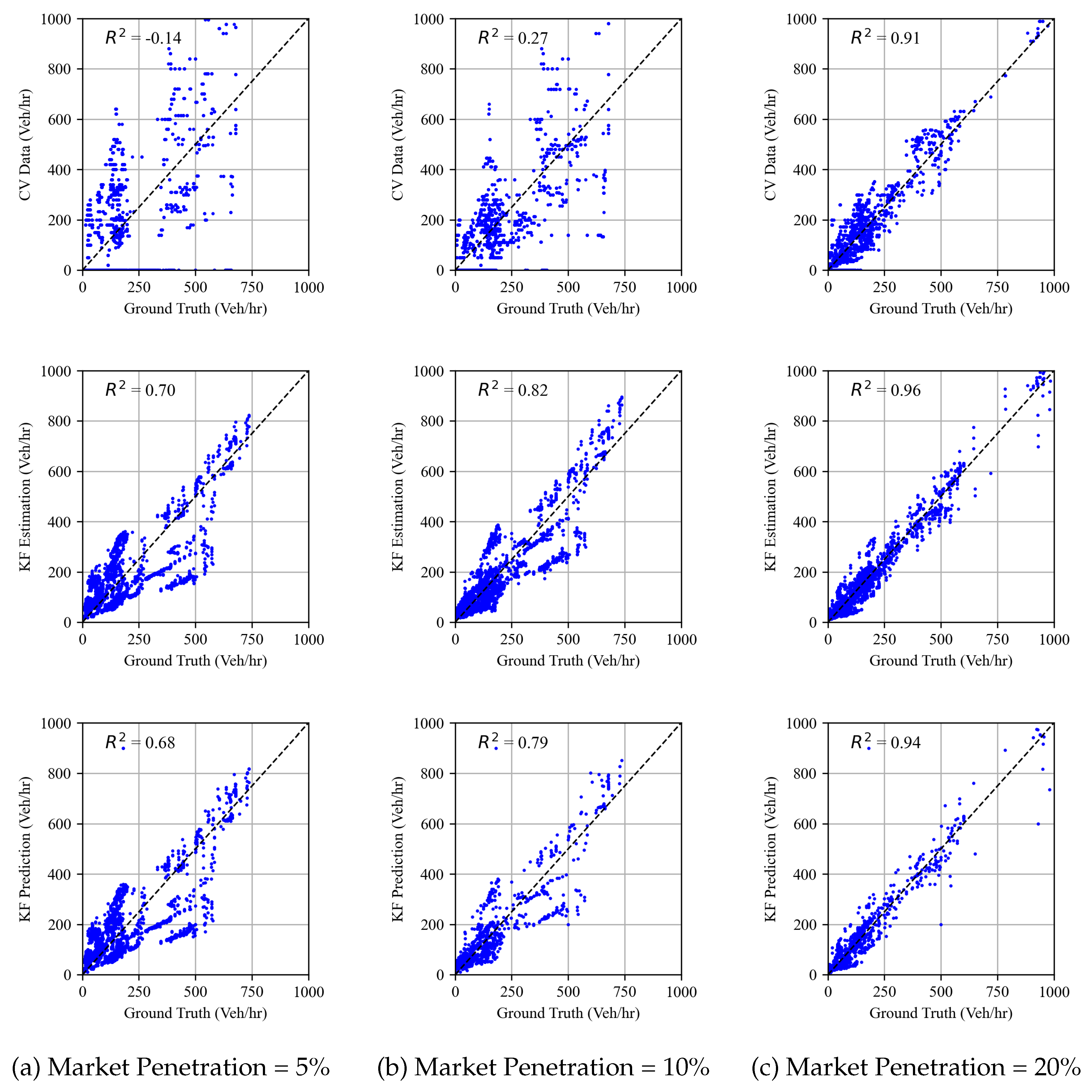
The findings were also evaluated by the results of the analysis depicted in Figure 7. For instance, at the 5% penetration level, the coefficient of determination advanced from white-0.14 for probe-vehicle-estimated TMs to a significantly improved white0.70 for Kalman filter-estimated TMs at a market penetration level of 5%. Moreover, the Kalman filter predictions exhibit a coefficient of determination of white0.68, which is a substantial enhancement over the accuracy achieved when using only probe vehicle data. These results illustrate the effectiveness of the Kalman filter approach in refining TM estimates and providing reliable TM estimates that are representative of real-time traffic dynamics.
Figure 8 shows the probability distribution of the difference between the ground-truth approach flows and the corresponding estimates/predictions generated by the Kalman filter algorithm. Notably, the deviations observed in TM estimates derived from probe vehicle data are significantly reduced. Furthermore, Figure 9 shows the root-mean-squared error (RMSE) values across various levels of CV market penetration implemented in this study. The outcomes reveal that the Kalman filter algorithm consistently outperforms solely CV-derived estimates in capturing the current system state. Furthermore, even at lower CV market penetration levels, the Kalman filter algorithm demonstrates improved predictive capabilities for TM counts, with an RMSE value ranging from white164 to 27 vehicles/hr at various MP levels as shown in Figure 10, where the level of error is significantly less than the estimated TM by probe vehicle data solely. This underlines the reliability of the proposed Kalman filter approach, which qualifies this algorithm to be used as a tool to provide TM counts for queue size estimation algorithms, as performed in this research. The algorithm also qualifies to be integrated with real-time traffic analysis and signal control systems, with varying degrees of CV market penetration levels.
6.2.2. Validation of INTEGRATION Micro-Simulation Model
To validate the input demand, Figure 11 shows that the simulated loop detector data match the observed demands derived from the raw trajectory data (). Furthermore, to validate the use of this model for further queuing analysis, the Kalman filter TM estimation approach was applied to both the simulated outputs and the raw trajectory data. Figure 12 shows a comparison between the RMSE of both estimates using raw trajectory data versus the INTEGRATION model output trajectory dataset. The figure shows high consistency between both outputs. The minor difference is due to the raw data’s higher resolution of vehicle trajectory data (30 frames per second versus the simulated data of 1 frame per second), which translates into more randomness and higher estimation error, as shown in the figure. These results enable us to confidently evaluate the proposed queue estimation scheme using the developed microscopic simulation model data.
6.3. Queue Size and Density Estimation Results
In this subsection, the lower level of the proposed approach is evaluated. The Kalman filter method was used for queue size and density estimation and compared with the baseline estimates using solely probe vehicle data. The TM estimates conducted at the upper level were utilized to estimate and predict the real-time queue size and density. The lower level approach was implemented for the isolated signalized intersection for multiple levels of probe vehicle penetration ranging from 5% to 100% for each prediction horizon of 5 and 10 seconds.
Figure 13 shows the queue size estimation results for the through and left TMs at the north-bound (NB) approach of the intersection for market penetration levels of 5%, 10%, and 20%, respectively. The figure shows the performance of the queue estimation algorithm using Kalman filters, where it captures the general queuing pattern, even at low levels of market penetration. The estimation accuracy is further quantified in Figure 14, which shows the performance of the proposed estimation scheme at various levels of market penetration ranging from 5% to 100%. Mean absolute percentage error (MAPE) and the mean absolute error (MAE) are the measures of performance (MOP) chosen for evaluation.
Figure 14 illustrates the performance evaluation results of the queue estimation and prediction. The figure shows that the use of Kalman filtering for queue size estimation outperforms the baseline estimates using the probe vehicle data by up to white32.8%, which highlights the filter’s capability to reduce the estimation noise at low levels of market penetration. However, at high levels of market penetration, the results show an insignificant impact from using Kalman filters compared to the sole use of probe vehicle data to derive queue size estimates. The figure also shows the prediction quantification results, where the level of error is consistent with the state estimation error results across various MP levels.
To quantify the estimation of upstream traffic density, Figure 15 shows the MAE of the traffic density estimates (the number of vehicles traveling at upstream links) and predictions using Kalman filters compared to the baseline method. The figure shows improved estimation at various market penetration levels, where the MAE improved by up to white18.5%. The figure also shows the prediction performance of the filter, whose prediction accuracy is consistent with the estimation accuracy.
6.4. Discussion
The previous subsections demonstrated the efficiency of the proposed bi-level approach for TM, density, and queue size estimation and prediction using Kalman filters. The proposed system showed enhanced state estimation and prediction and it’s applicability for field implementation and integration with traffic signal control systems. Specifically, the proposed bi-level approach improved traffic state estimates and predictions producing significant system performance at low levels of market penetration. However, the results showed a comparatively marginal enhancement achieved by the proposed approach at higher penetration levels compared to the baseline. This is attributed to the increased accuracy and reduced noise inherent in the probe vehicle data at higher penetration levels, diminishing the necessity for the noise reduction process carried out by the Kalman filter. As such, this research suggests using Kalman filters to enhance state estimates when the market penetration level is below 30%. These findings are consistent with the literature, where Aljamal et al. [39] showed similar findings, where the authors used Kalman filters to estimate the total number of vehicle counts at intersection approaches using probe vehicle data. The results of this paper also confirm the ability of Kalman filters to enhance the estimation of various traffic states such as turning movements, vehicle queues, and traffic stream density.
Furthermore, this research addresses the limitations of traffic state estimation and prediction techniques found in the literature using probe data, such as machine-learning techniques [40]. Machine learning models typically require historical traffic data and extensive computational resources for training, and they are prone to over-fitting, which compromises their predictive accuracy. The bi-level approach proposed in this research demonstrates enhanced estimation and prediction accuracy without the need for historical traffic data. Furthermore, it exhibits computational efficiency suitable for real-time applications. This research also advances the literature in employing Kalman filters in short-term and real-time traffic state estimation without the need for historical traffic data, which might be unavailable in many cases.
In addition, the presented prediction capability is considered a useful prediction tool for integration into advanced traffic signal control systems, such as the adaptive traffic signal controller proposed by Abdelghafar et al. [2], which requires real-time predictions of TM counts, queue sizes as well as traffic density estimates for each TM at each approach. Due to the lack of this information in previous research, the proposed system was only tested considering market penetration levels of 100%. However, the assumed high level of market penetration is inconsistent with the current penetration trends, which makes this system inapplicable in the field. The bi-level approach proposed in this research fills the gap in previous research to develop the adaptive game-theoretic system, which requires real-time traffic state estimation and prediction. The availability of this information allows for further deployment and testing of its efficiency at low levels of market penetration. Furthermore, the queue estimation performance shows its efficiency in being integrated into vehicle trajectory optimization systems, in which the real-time position of the back of the queue is essential for vehicle trajectory optimization in the vicinity of traffic signals [41,42]
7. Conclusions and Future Directions
This paper introduces a bi-level approach that leverages probe vehicle and upstream detector data for real-time traffic state estimation and prediction. A Kalman filter approach is utilized to provide enhanced traffic state estimates compared to those provided solely by probe vehicle data. In the upper level, the number of turning vehicles is estimated in real time, and in the lower level, the upstream link density and the number of queued vehicles at the intersection, categorized by movement, are estimated. A sampling error analysis is utilized to estimate the error covariance matrices for the Kalman filter measurements and predictions using real-time data. The proposed system is evaluated using a drone-collected dataset at a four-legged signalized intersection in Orlando, Florida.
Implementation results show that the proposed methodology has demonstrated promising results in enhancing traffic state estimation and prediction capabilities, in terms of turning movements, queue size, and upstream link density. In the upper level, the TM estimation results show a reduction in the error SD of up to white50% relative to the baseline method relying solely on probe vehicle data. The of the TM estimates is significantly improved by using Kalman filters from white0.14 to 0.70 at a market penetration of 5%. Similarly, at a market penetration of 10%, the improved from white0.27 to 0.82. Furthermore, the upper level showed reliable prediction capability with values of white0.68, 0.79, and 0.94 for market penetration levels of white5%, 10%, and 20%, respectively.
In the lower level, the queue size and upstream link density are estimated using Kalman filters utilizing TM estimates provided in the upper level and probe vehicle data. Results of the queue size estimation showed enhanced estimation accuracy at lower levels of market penetration. Comparing the estimated queue size with the actual, the MAPE was enhanced with up to white32.8%. In addition, the lower level filter produced enhanced estimates of upstream traffic density of up to white18.5%. The proposed approach also shows enhanced estimation and prediction performance at a lower level of market penetration.
The research indicates its applicability for field implementation and integration with real-time game-theoretic traffic signal control systems, even at low levels of market penetration. This approach addresses the limitations of existing techniques, such as machine learning models, by providing enhanced accuracy without the need for historical traffic data and with computational efficiency suitable for real-time applications. Moreover, the prediction capability of this algorithm presents a valuable tool for integration into vehicle trajectory optimization systems. Overall, this research fills a crucial gap in previous studies and paves the way for the development and testing of efficient systems at various levels of market penetration, ultimately contributing to the advancement of traffic management and optimization.
Future directions for research include enhancement of the propoesed system by integrating a more sophisticated approach for the market penetration rate estimation, rather than the simple method currently used in the system. Furthermore, future directions also include the integration of the proposed KF approach within an adaptive game-theoretic traffic signal controller; as such, categorized traffic state estimates can be provided to the controller at various market penetration conditions. Therefore, the controller will be suitable for field implementation.
Author Contributions
Conceptualization, H.A.R., and A.K.S.; methodology, H.A.R., and A.K.S.; software, A.K.S.; validation, A.K.S., and H.A.R.; formal analysis, A.K.S., and H.A.R.; data curation, A.K.S.; writing—original draft preparation, A.K.S.; writing—review and editing, H.A.R.; visualization, A.K.S. All authors have read and agreed to the published version of the manuscript.
Funding
This research was funded by Sustainable Mobility and Accessibility Regional Transportation Equity Research Center, Morgan State University.
Institutional Review Board Statement
Not applicable.
Informed Consent Statement
Not applicable.
Acknowledgments
This effort was funded by the Sustainable Mobility and Accessibility Regional Transportation Equity Research (SMARTER) Center.
Conflicts of Interest
The authors declare no conflicts of interest. The funders had no role in the design of the study; in the collection, analyses, or interpretation of data; in the writing of the manuscript; or in the decision to publish the results.
Abbreviations
The following abbreviations are used in this manuscript:
| TSC | Traffic Signal Control |
| DNB | Decentralized nash Bargaining |
| VOC | Volume-Capacity Ratio |
References
- Blokpoel, R.; Vreeswijk, J. Uses of Probe Vehicle Data in Traffic Light Control. Transportation Research Procedia 2016, 14, 4572–4581. [Google Scholar] [CrossRef]
- Abdelghaffar, H.M.; Rakha, H.A. Development and Testing of a Novel Game Theoretic De-Centralized Traffic Signal Controller. IEEE Transactions on Intelligent Transportation Systems 2021, 22, 231–242. [Google Scholar] [CrossRef]
- Schaefer, M.C. Estimation of Intersection Turning Movements from Approach Counts. Ite Journal-institute of Transportation Engineers.
- Hauer, E.; Pagitsas, E.; Shin, B.T. Estimation of Turning Flows from Automatic Counts. Transportation Research Record 1981, 795. [Google Scholar]
- Van Aerde, M.; Rakha, H.; Paramahamsan, H. Estimation of Origin-Destination Matrices: Relationship Between Practical and Theoretical Considerations. Transportation Research Record: Journal of the Transportation Research Board 2003, 1831, 122–130. [Google Scholar] [CrossRef]
- Xu, K.; Yi, P.; Shao, C.; Mao, J.; Xu, K.; Yi, P.; Shao, C.; Mao, J. Development and Testing of an Automatic Turning Movement Identification System at Signalized Intersections. Journal of Transportation Technologies 2013, 3, 241–246. [Google Scholar] [CrossRef]
- Zhang, X.; Cai, X.; Sun, L. Estimation of Intersection Turning Movement Proportions Using MATLAB. CICTP 2012: Multimodal Transportation Systems - Convenient, Safe, Cost-Effective, Efficient - Proceedings of the 12th COTA International Conference of Transportation Professionals, A: 822–828. ISBN: 9780784412442 Publisher, 9780. [Google Scholar] [CrossRef]
- Chen, A.; Chootinan, P.; Ryu, S.; Lee, M.; Recker, W. An intersection turning movement estimation procedure based on path flow estimator. Journal of Advanced Transportation 2012, 46, 161–176. [Google Scholar] [CrossRef]
- Jiao, P.; Huapu, L.U.; Yang, L. Real-time estimation of turning movement proportions based on genetic algorithm. IEEE Conference on Intelligent Transportation Systems, Proceedings, ITSC 2005, 2005, 484–489. [Google Scholar] [CrossRef]
- Ghanim, M.S.; Shaaban, K. Estimating Turning Movements at Signalized Intersections Using Artificial Neural Networks. IEEE Transactions on Intelligent Transportation Systems 2019, 20, 1828–1836. [Google Scholar] [CrossRef]
- Mousavizadeh, O.; Keyvan-Ekbatani, M.; Logan, T.M. Real-time turning rate estimation in urban networks using floating car data. Transportation Research Part C: Emerging Technologies 2021, 133, 103457. [Google Scholar] [CrossRef]
- Lan, C.J.; Davis, G.A. Real-time estimation of turning movement proportions from partial counts on urban networks. Transportation Research Part C: Emerging Technologies 1999, 7, 305–327. [Google Scholar] [CrossRef]
- Mirchandani, P.B.; Nobe, S.A.; Wu, W.W. Online Turning Proportion Estimation in Real-Time Traffic-Adaptive Signal Control. Transportation Research Record 2001, 1748, 80–86. [Google Scholar] [CrossRef]
- Saldivar-Carranza, E.D.; Li, H.; Bullock, D.M. Identifying Vehicle Turning Movements at Intersections from Trajectory Data. IEEE Conference on Intelligent Transportation Systems, Proceedings, ITSC, I: 4043–4050. ISBN: 9781728191423 Publisher, 4043. [Google Scholar] [CrossRef]
- Wei, L.; Li, J.h.; Xu, L.w.; Gao, L.; Yang, J. Queue Length Estimation for Signalized Intersections under Partially Connected Vehicle Environment. Journal of Advanced Transportation 2022, 2022, 1–11. [Google Scholar] [CrossRef]
- Comert, G.; Cetin, M. Analytical Evaluation of the Error in Queue Length Estimation at Traffic Signals From Probe Vehicle Data. IEEE Transactions on Intelligent Transportation Systems 2011, 12, 563–573. [Google Scholar] [CrossRef]
- Liu, H.; Liang, W.; Rai, L.; Teng, K.; Wang, S. A Real-Time Queue Length Estimation Method Based on Probe Vehicles in CV Environment. IEEE Access 2019, 7, 20825–20839. [Google Scholar] [CrossRef]
- Zhao, Y.; Zheng, J.; Wong, W.; Wang, X.; Meng, Y.; Liu, H.X. Various methods for queue length and traffic volume estimation using probe vehicle trajectories. Transportation Research Part C: Emerging Technologies 2019, 107, 70–91. [Google Scholar] [CrossRef]
- Rostami-Shahrbabaki, M.; Safavi, A.A.; Papageorgiou, M.; Setoodeh, P.; Papamichail, I. State estimation in urban traffic networks: A two-layer approach. Transportation Research Part C: Emerging Technologies 2020, 115, 102616. [Google Scholar] [CrossRef]
- Hao, P.; Ban, X.J.; Guo, D.; Ji, Q. Cycle-by-cycle intersection queue length distribution estimation using sample travel times. Transportation Research Part B: Methodological 2014, 68, 185–204. [Google Scholar] [CrossRef]
- van Lint, H.; Djukic, T. Applications of Kalman Filtering in Traffic Management and Control. In New Directions in Informatics, Optimization, Logistics, and Production; INFORMS TutORials in Operations Research, INFORMS, 2012; pp. 59–91. 4: Section; 4. [CrossRef]
- Aljamal, M.A.; Abdelghaffar, H.M.; Rakha, H.A. Kalman Filter-based Vehicle Count Estimation Approach Using Probe Data: A Multi-lane Road Case Study. In Proceedings of the 2019 IEEE Intelligent Transportation Systems Conference (ITSC); 2019; pp. 4374–4379. [Google Scholar] [CrossRef]
- Antoniou, C.; Ben-Akiva, M.; Koutsopoulos, H.N. Nonlinear Kalman Filtering Algorithms for On-Line Calibration of Dynamic Traffic Assignment Models. IEEE Transactions on Intelligent Transportation Systems 2007, 8, 661–670. [Google Scholar] [CrossRef]
- Emami, A.; Sarvi, M.; Asadi Bagloee, S. Using Kalman filter algorithm for short-term traffic flow prediction in a connected vehicle environment. Journal of Modern Transportation 2019, 27, 222–232. [Google Scholar] [CrossRef]
- Wang, Y.; Papageorgiou, M.; Messmer, A. Real-Time Freeway Traffic State Estimation Based on Extended Kalman Filter: A Case Study. Transportation Science 2007, 41, 167–181. [Google Scholar] [CrossRef]
- Bekiaris-Liberis, N.; Roncoli, C.; Papageorgiou, M. Highway Traffic State Estimation With Mixed Connected and Conventional Vehicles. IEEE Transactions on Intelligent Transportation Systems 2016, 17, 3484–3497. [Google Scholar] [CrossRef]
- Jiao, P.; Sun, T.; Du, L. A Bayesian Combined Model for Time-Dependent Turning Movement Proportions Estimation at Intersections. Mathematical Problems in Engineering 2014, 2014. [Google Scholar] [CrossRef]
- Zhang, H.; Poschinger, A. Estimation of Turning Ratio at Intersections Based on Detector Data using Kalman Filter. Transportation Research Procedia 2019, 41, 673–687. [Google Scholar] [CrossRef]
- Enjedani, S.N.; Khanal, M. Development of a Turning Movement Estimator Using CV Data. Future Transportation 2023, Vol. 3, Pages 349-367 2023, 3, 349–367. [Google Scholar] [CrossRef]
- Hu, S.; Zhou, Q.; Li, J.; Wang, Y.; Roncoli, C.; Zhang, L.; Lehe, L. High Time-Resolution Queue Profile Estimation at Signalized Intersections Based on Extended Kalman Filtering. IEEE Transactions on Intelligent Transportation Systems 2022, 23, 21274–21290. [Google Scholar] [CrossRef]
- Kalman, R.E. A New Approach to Linear Filtering and Prediction Problems. Journal of Basic Engineering 1960, 82, 35–45. [Google Scholar] [CrossRef]
- Auger, F.; Hilairet, M.; Guerrero, J.M.; Monmasson, E.; Orlowska-Kowalska, T.; Katsura, S. Industrial applications of the kalman filter: A review. IEEE Transactions on Industrial Electronics 2013, 60, 5458–5471. [Google Scholar] [CrossRef]
- Cao, J.; Hu, D.; Hadiuzzaman, M.; Wang, X.; Qiu, T.Z. Comparison of queue estimation accuracy by shockwave-based and input-output-based models. In Proceedings of the 17th International IEEE Conference on Intelligent Transportation Systems (ITSC); 2014; pp. 2687–0017. [Google Scholar] [CrossRef]
- Zheng, O.; Abdel-Aty, M.; Yue, L.; Abdelraouf, A.; Wang, Z.; Mahmoud, N. CitySim: A Drone-Based Vehicle Trajectory Dataset for Safety-Oriented Research and Digital Twins. Transportation Research Record. [CrossRef]
- Van Aerde, M.; Hellinga, B.; Baker, M.; Rakha, H. INTEGRATION : An Overview of Traffic Simulation Features, Washington, D.C., 1998.
- Farag, M.M.G.; Rakha, H.A.; Mazied, E.A.; Rao, J. INTEGRATION Large-Scale Modeling Framework of Direct Cellular Vehicle-to-All (C-V2X) Applications. Technical report, 2021. Number: 6 Publisher: Multidisciplinary Digital Publishing Institute.
- Rakha, H. INTEGRATION © RELEASE 2.40 FOR WINDOWS: User’s Guide – Volume I: Fundamental Model Features. Technical report, 2020. Publisher: Virginia Polytechnic Institute and State University Version Number: 1.
- Rakha, H. INTEGRATION © RELEASE 2.40 FOR WINDOWS: User’s Guide – Volume II: Advanced Model Features; 2020. [CrossRef]
- Aljamal, M.A.; Abdelghaffar, H.M.; Rakha, H.A. Real-Time Estimation of Vehicle Counts on Signalized Intersection Approaches Using Probe Vehicle Data. IEEE Transactions on Intelligent Transportation Systems 2021, 22, 2719–2729. [Google Scholar] [CrossRef]
- Sekuła, P.; Marković, N.; Vander Laan, Z.; Sadabadi, K.F. Estimating historical hourly traffic volumes via machine learning and vehicle probe data: A Maryland case study. Transportation Research Part C: Emerging Technologies 2018, 97, 147–158. [Google Scholar] [CrossRef]
- Shafik, A.K.; Eteifa, S.; Rakha, H.A. Optimization of Vehicle Trajectories Considering Uncertainty in Actuated Traffic Signal Timings. IEEE Transactions on Intelligent Transportation Systems 2023, 24, 7259–7269. [Google Scholar] [CrossRef]
- Shafik, A.; Rakha, H.A. Queue Length Estimation and Optimal Vehicle Trajectory Planning Considering Queue Effects at Actuated Traffic Signal Controlled Intersections 2024.
Figure 1.
Kalman Filter Process
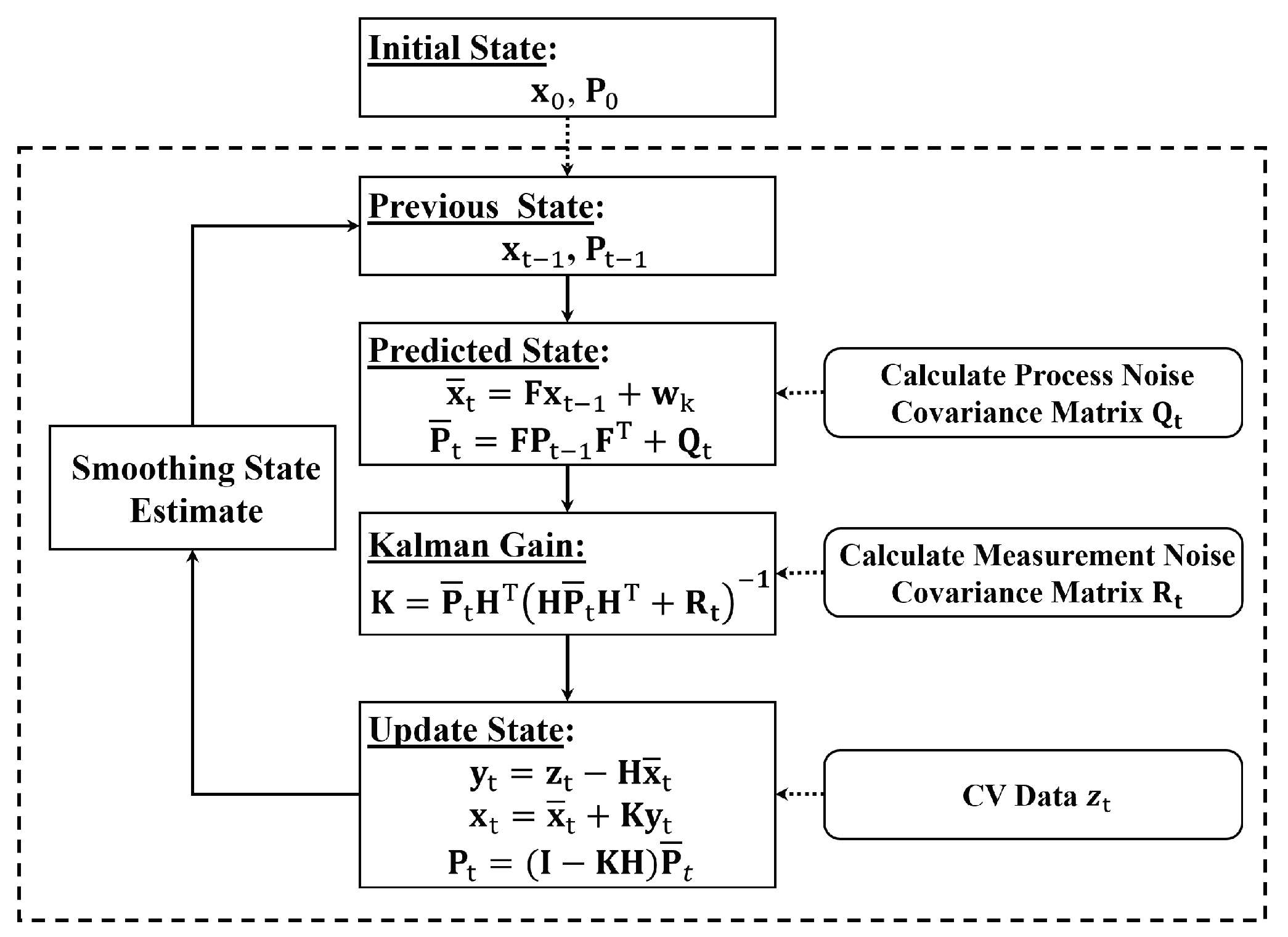
Figure 2.
Four-legged Signalized Intersection at Alafaya Trail and University Boulevard in Orlando, Florida.
Figure 2.
Four-legged Signalized Intersection at Alafaya Trail and University Boulevard in Orlando, Florida.
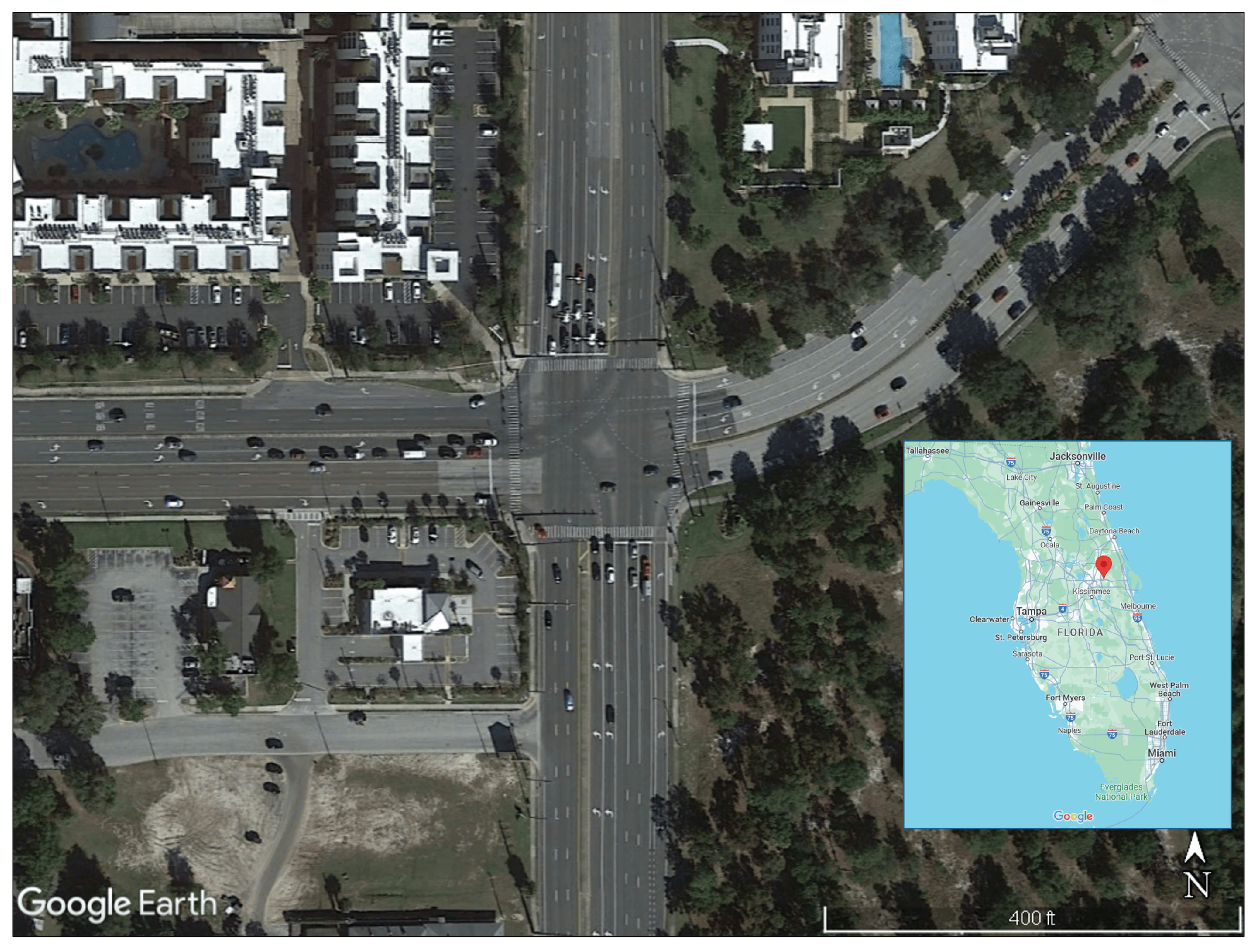
Figure 3.
Snapshot of INTEGRATION Microscopic Simulation Model.
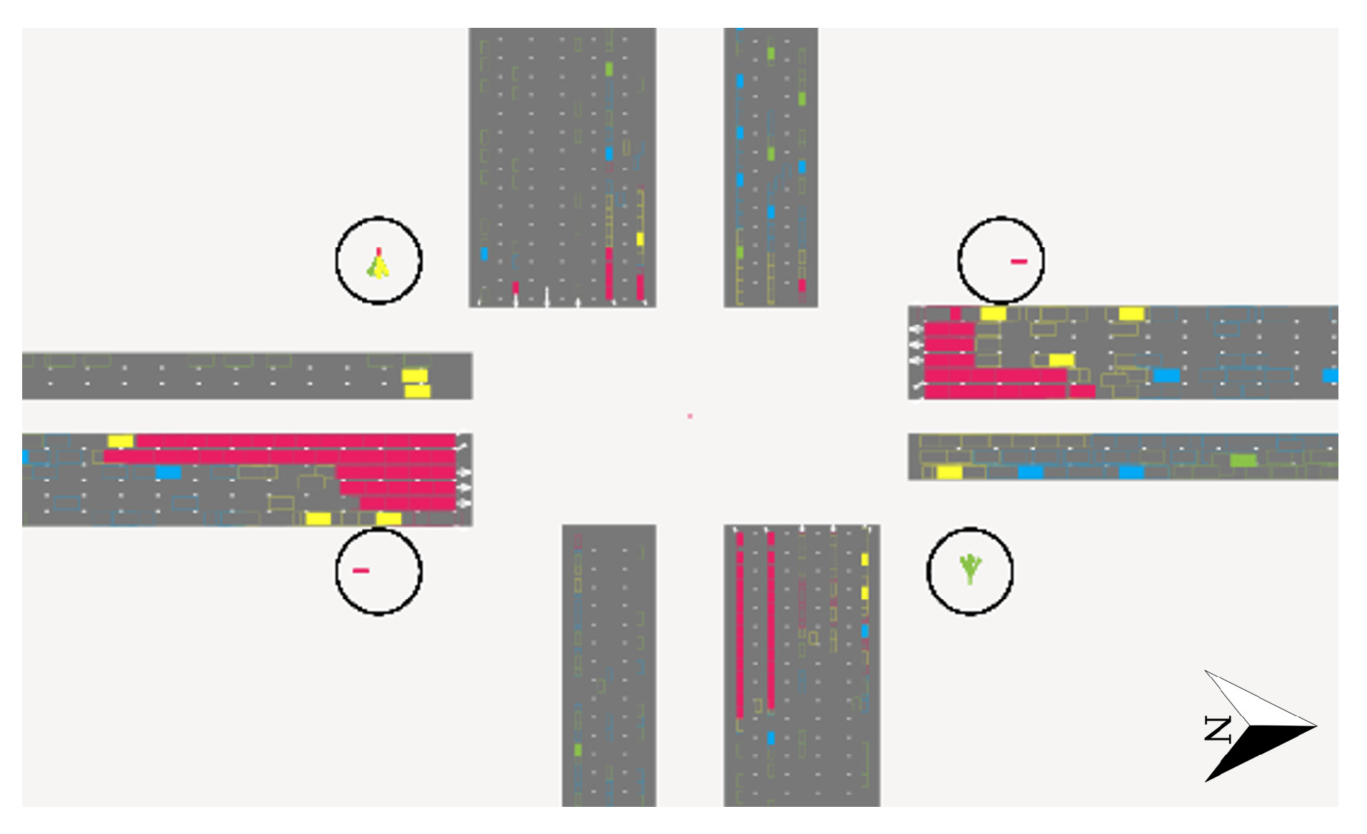
Figure 4.
Comparison Between Kalman Filter-Derived TM Counts Versus CV Observations and Ground Truth Counts for the EB Approach at Market Penetration = 5%.
Figure 4.
Comparison Between Kalman Filter-Derived TM Counts Versus CV Observations and Ground Truth Counts for the EB Approach at Market Penetration = 5%.
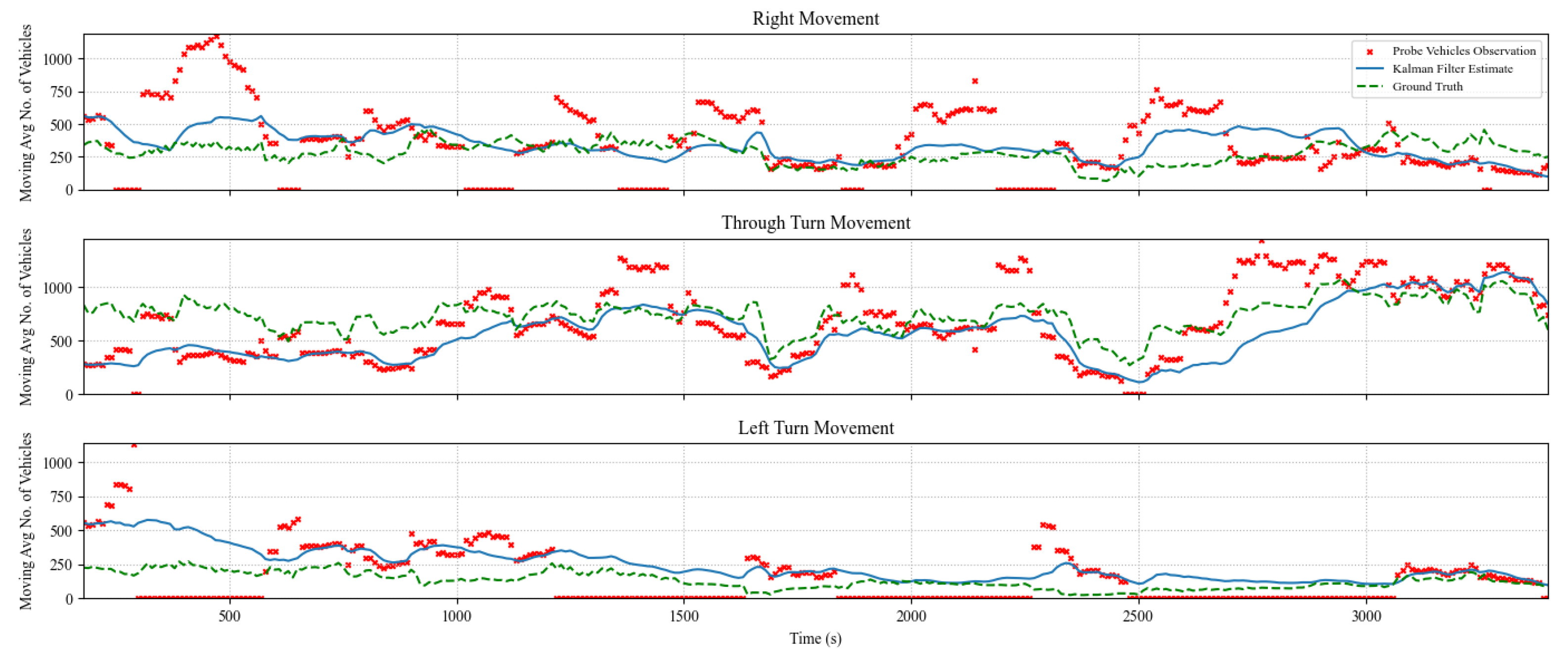
Figure 5.
Comparison Between Kalman Filter-Derived TM Counts Versus CV Observations and Ground Truth Counts for the EB Approach at Market Penetration = 10%.
Figure 5.
Comparison Between Kalman Filter-Derived TM Counts Versus CV Observations and Ground Truth Counts for the EB Approach at Market Penetration = 10%.
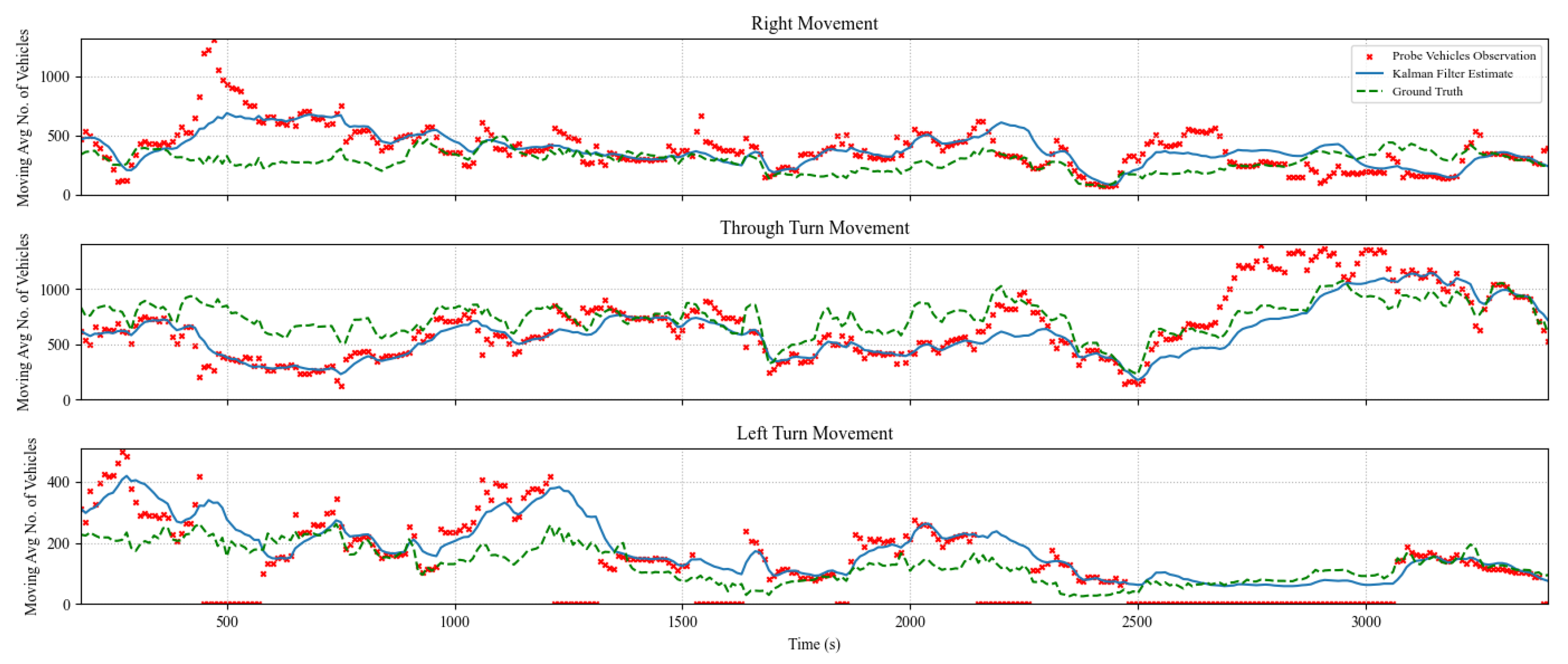
Figure 6.
Comparison Between Kalman Filter-Derived TM Counts Versus CV Observations and Ground Truth Counts for the EB Approach at Market Penetration = 20%.
Figure 6.
Comparison Between Kalman Filter-Derived TM Counts Versus CV Observations and Ground Truth Counts for the EB Approach at Market Penetration = 20%.
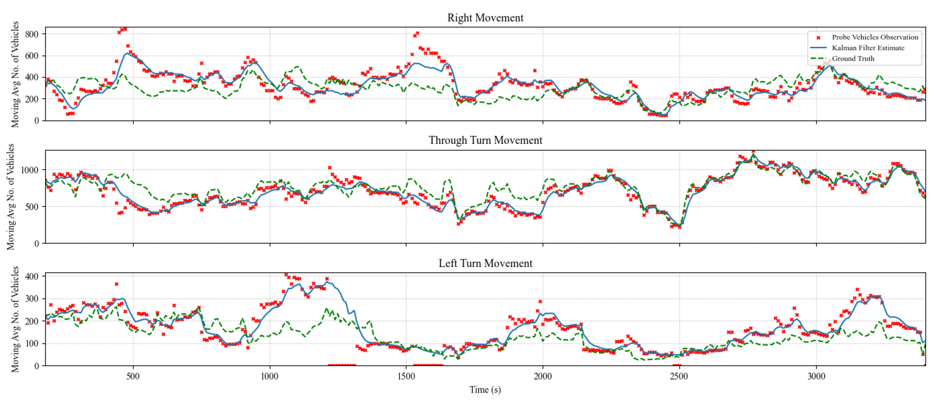
Figure 7.
Correspondence Between TM Estimates and Ground Truth.
| (a) Market Penetration = 5% | (b) Market Penetration = 10% | (c) Market Penetration = 20% |
Figure 8.
The Cumulative Probability of the Difference Between the Ground Truth and Kalman Filter-Derived Estimated Flows.
Figure 8.
The Cumulative Probability of the Difference Between the Ground Truth and Kalman Filter-Derived Estimated Flows.
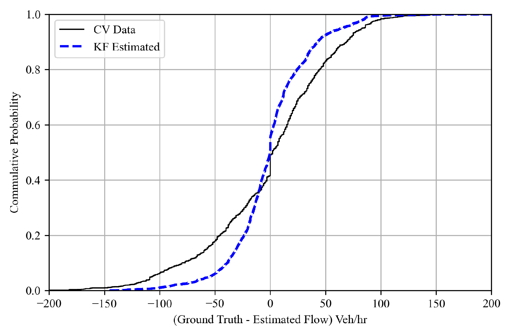
Figure 9.
TM Estimation Accuracy Results for Different Levels of Market Penetration.
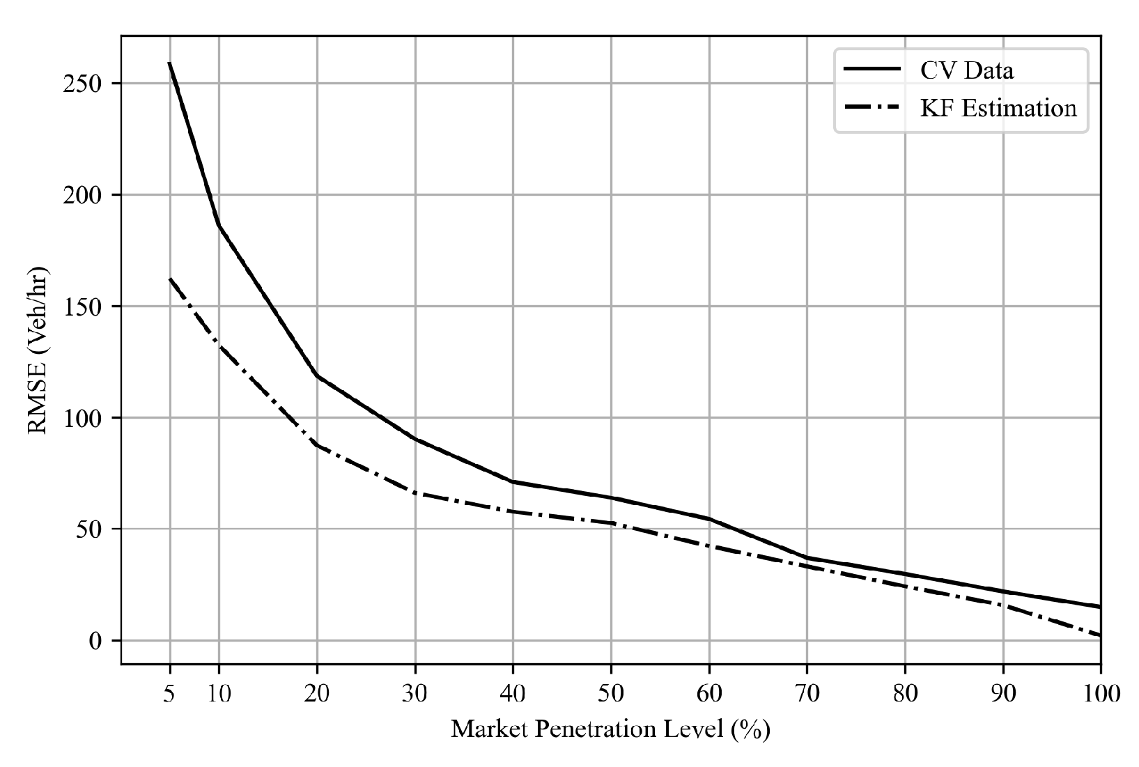
Figure 10.
TM Prediction RMSE Results for Different Levels of Market Penetration.
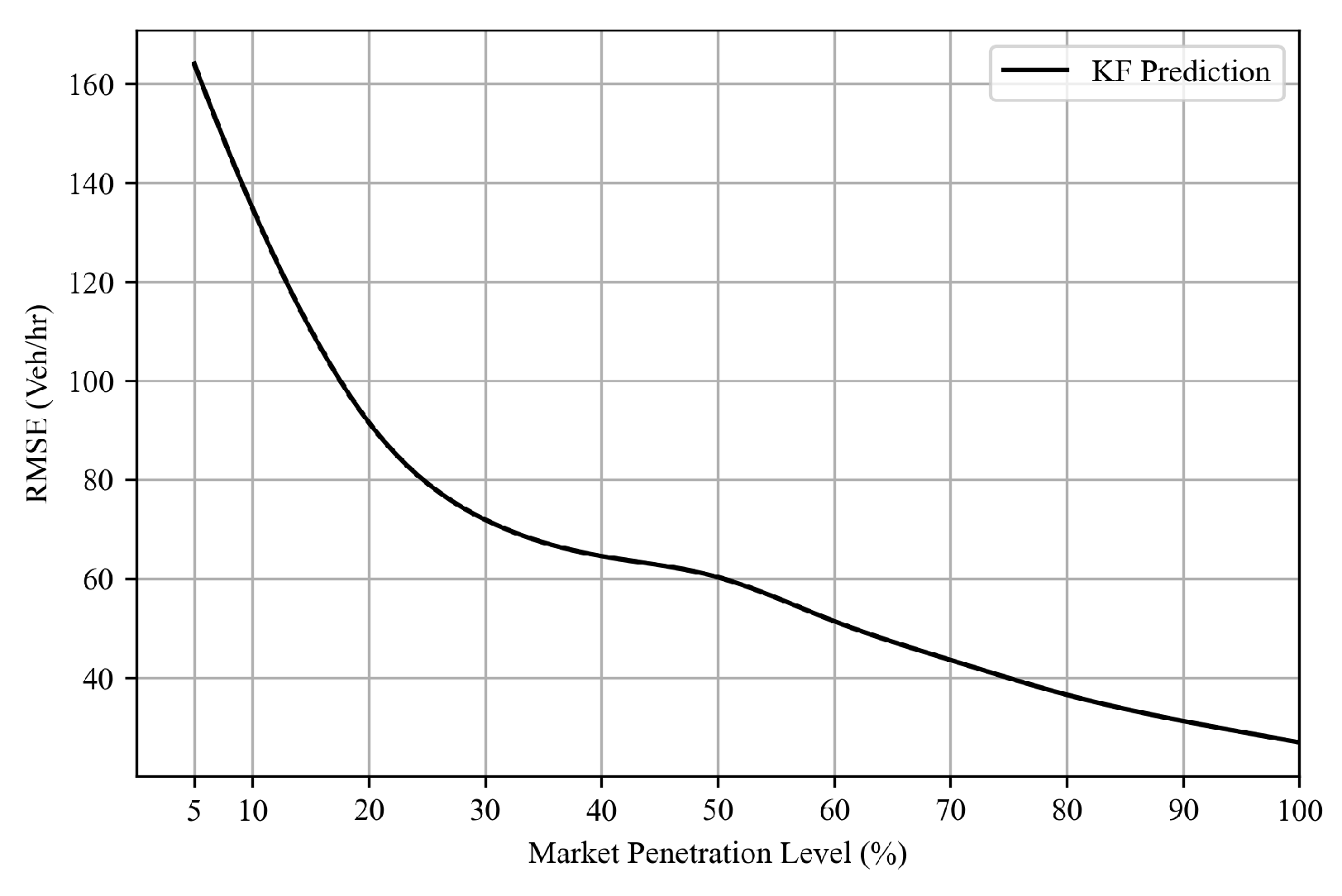
Figure 11.
Demand Validation.
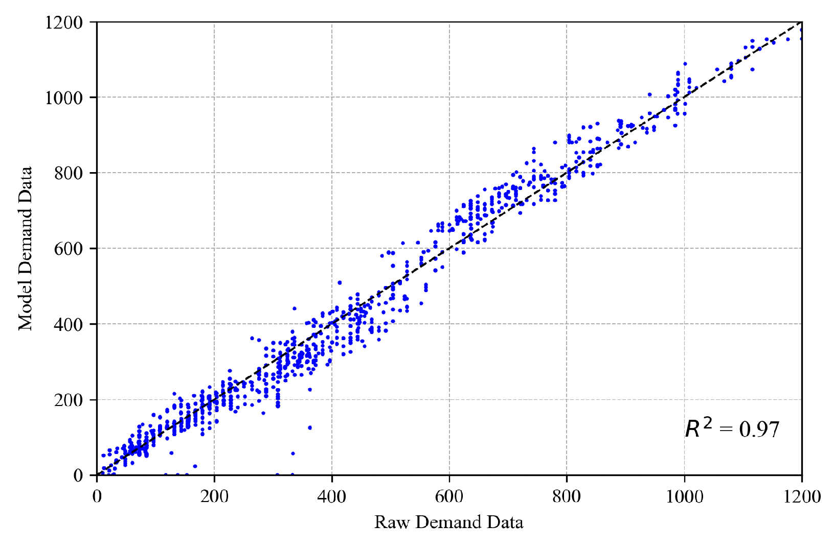
Figure 12.
Validation of the Developed INTEGRATION Microscopic Model.
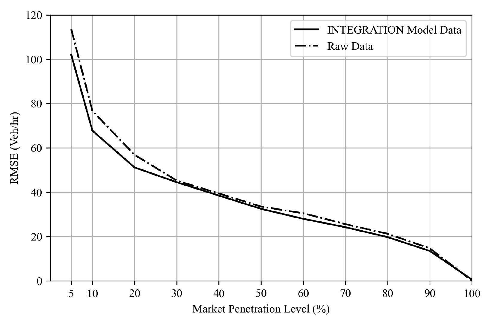
Figure 13.
Comparison Between Queue Estimation Using Kalman Filter Method and Ground Truth.
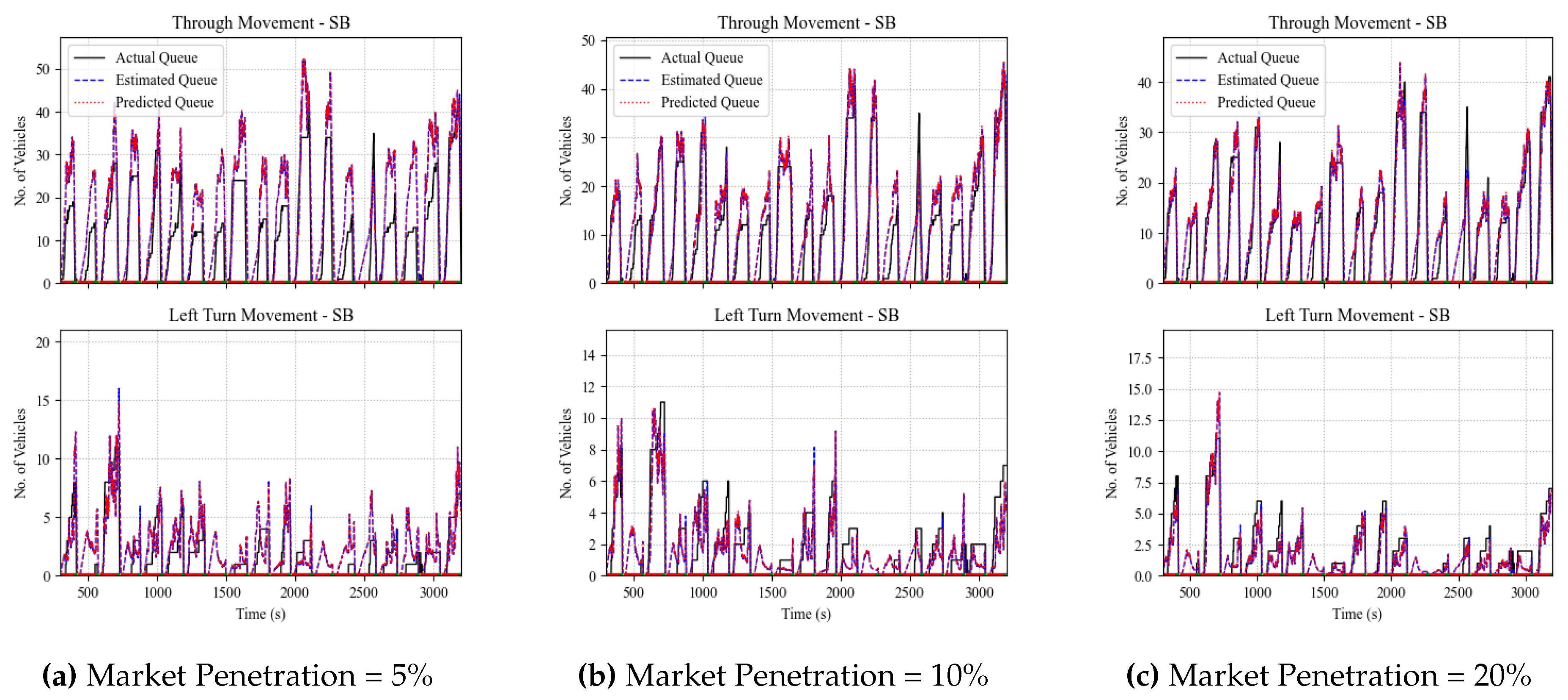
Figure 14.
Queue Estimation and Prediction MOP Results at Different Levels of Market Penetration.
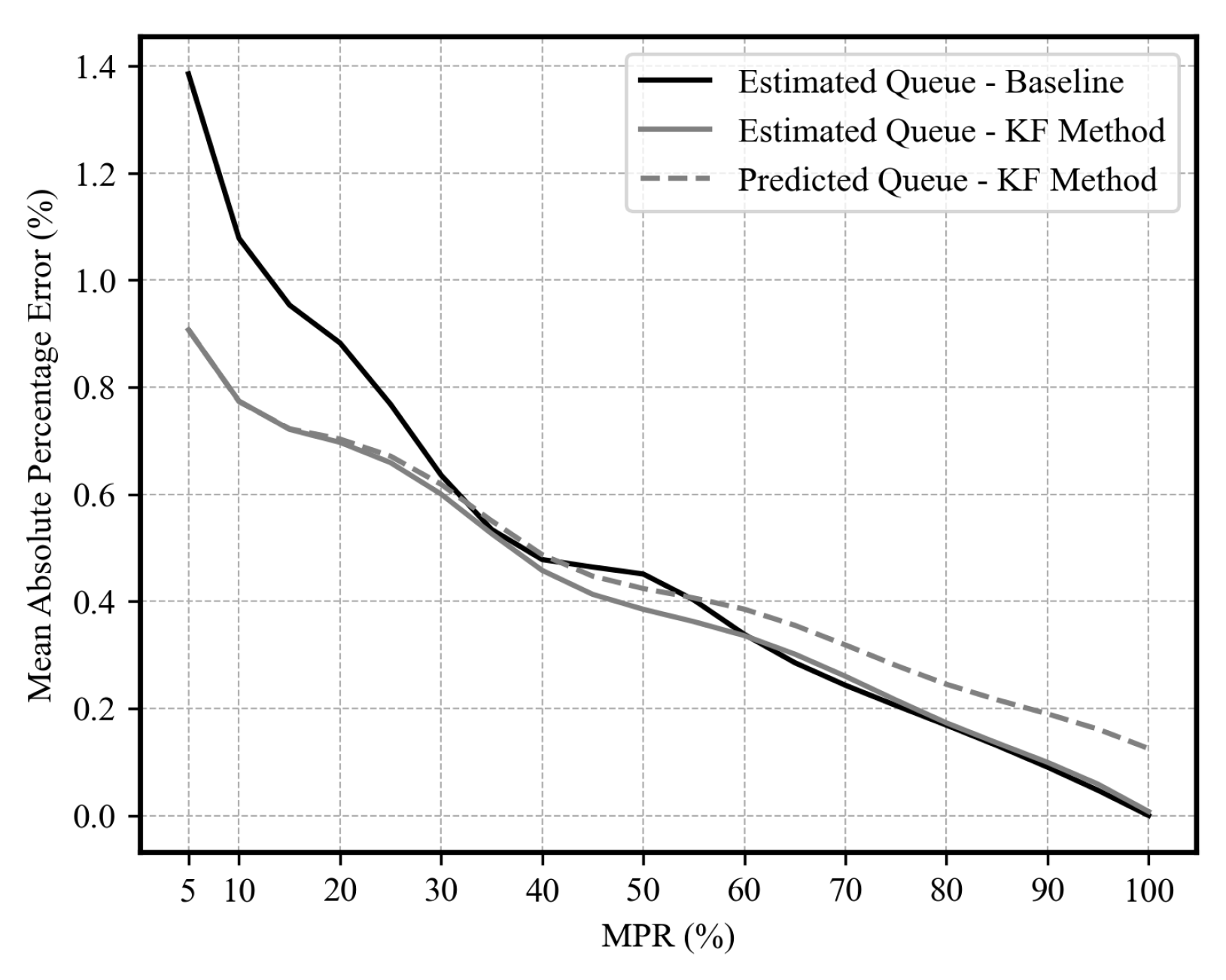
Figure 15.
Density Estimation and Prediction MOP Results at Different Levels of Market Penetration.
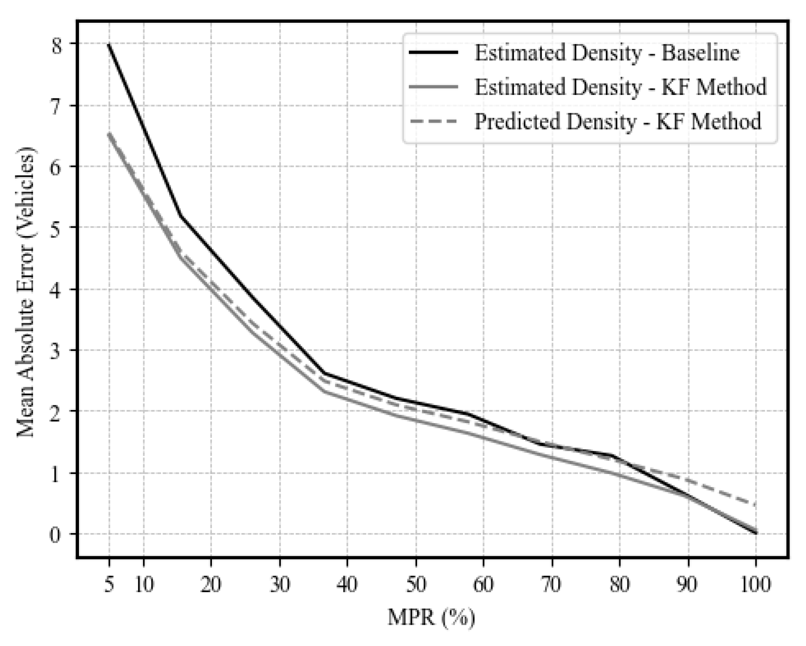

Table 1.
Intersection demand rate in vehicles/hr according to the drone-based vehicle trajectories.
| Approach | LT | THR | RT |
|---|---|---|---|
| NB | 71 | 721 | 88 |
| SB | 188 | 806 | 100 |
| EB | 121 | 1223 | 134 |
| WB | 86 | 844 | 278 |
Table 2.
A Comparison Between the SD of TMs (vehicles/hr) Derived From Probe Vehicle Data and Using Kalman Filtering.
Table 2.
A Comparison Between the SD of TMs (vehicles/hr) Derived From Probe Vehicle Data and Using Kalman Filtering.
| Approach | Market Penetration Levels | ||
|---|---|---|---|
| 5% | 10% | 20% | |
| SD of Probe Vehicle-Estimated TMs | 174.1 | 138.8 | 56.1 |
| SD of Kalman Filter-Estimated TMs | 90.5 | 69.1 | 35.9 |
| Estimation Improvement | 48.0% | 50.1% | 36.0% |
| SD of Kalman Filter-Predicted TMs | 92.8 | 72.5 | 42.7 |
Disclaimer/Publisher’s Note: The statements, opinions and data contained in all publications are solely those of the individual author(s) and contributor(s) and not of MDPI and/or the editor(s). MDPI and/or the editor(s) disclaim responsibility for any injury to people or property resulting from any ideas, methods, instructions or products referred to in the content. |
© 2024 by the authors. Licensee MDPI, Basel, Switzerland. This article is an open access article distributed under the terms and conditions of the Creative Commons Attribution (CC BY) license (https://creativecommons.org/licenses/by/4.0/).
Copyright: This open access article is published under a Creative Commons CC BY 4.0 license, which permit the free download, distribution, and reuse, provided that the author and preprint are cited in any reuse.


