1. Introduction
1.1. Fatigue Assessment for Long-Life Components
In the design of railway vehicles, their expected long longevity must always be taken into account. The essential components for the operation and safety of the railway vehicle must also be designed to operate for years, being only necessary to inspect and repair them [
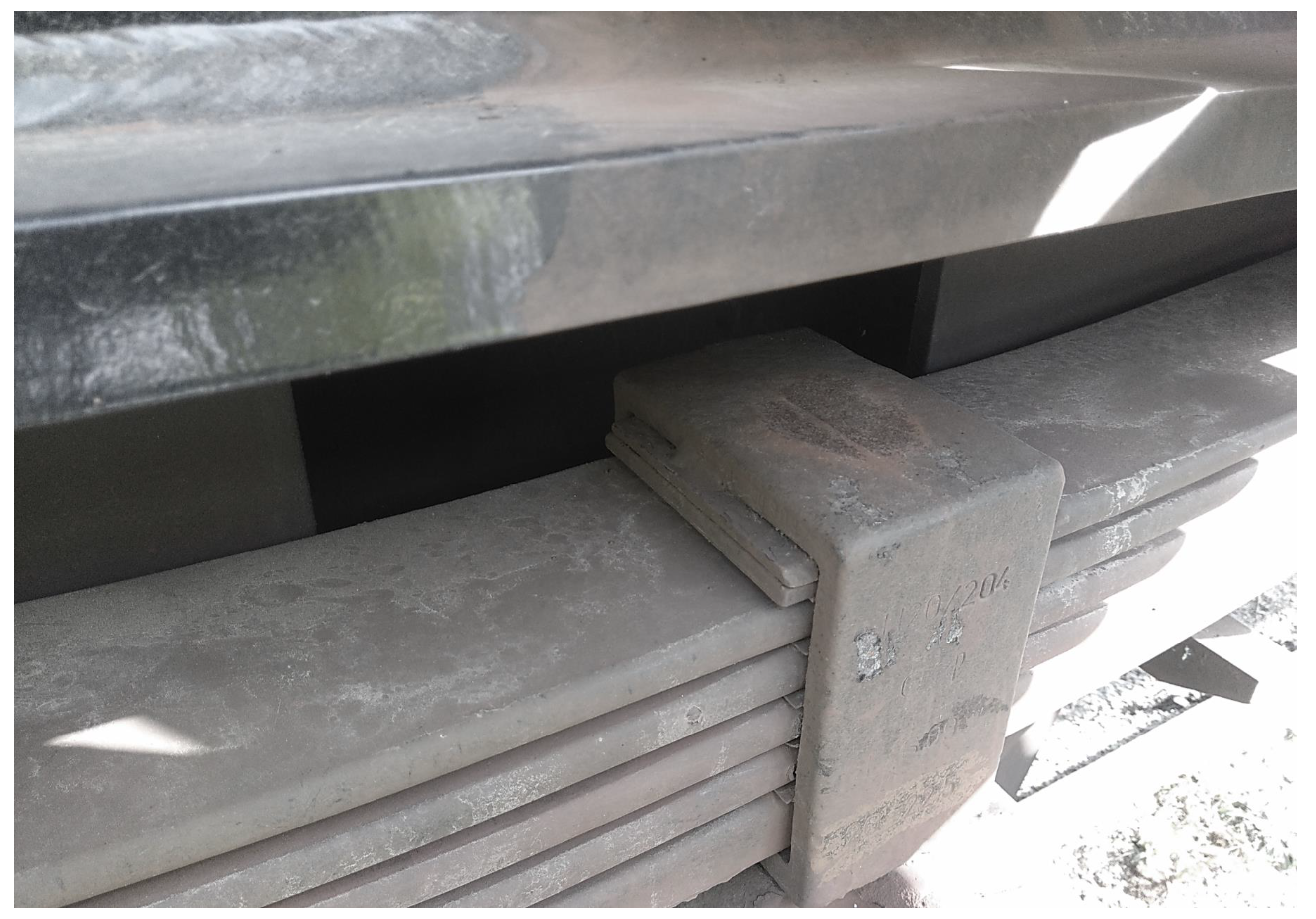
1]. Railway components such as axles, wheels, leaf springs (see
Figure 1), and bogies are some of the rail components designed to operate for a large number of cycles (
) [
2,
3,
4].
Fatigue tests have been performed for an endurance life of 10
6 or 10
7 cycles (often considered as run-out limit and infinite life), however, fatigue failures above this limit have been observed [
1,
2]. Within this range of endurance life, fatigue testing machines operating at 25 Hz are very time-consuming, which consequently forced the appearance of fast machines (operating at 10 times faster). Even so, these machines were not adequate to keep up with the evolution of science, which evolved for fatigue testing speeds up to 10
9 cycles. This fact motivated the development of ultrasonic fatigue testing machines that operate between 15 - 30 kHz (20 kHz, typically) [
5]. Effectively, the time needed to reach lives of 10
9 cycles is approximately 3 days (considering suitable stop-time for cooling). This new advance has raised interest in the scientific community for the study of failures motivated by fatigue cracks starting from internal inclusions and the hydrogen embrittlement effects [
6,
7].
1.2. Frequency Effect on Fatigue Behaviour of Metals
The frequency effect on fatigue resistance has also been analysed using ultrasonic fatigue testing machines. According to the literature, increasing frequency can positively affects the fatigue resistance of the material due to the strain rate effect on changing mechanical properties may exhibit insensitivity to the frequency [
8,
9,
10], however it might not have any effect of the fatigue strength or it might reduce it in some materials [
5]. For materials exhibiting an increasing in the fatigue strength with the frequency level, for example, for higher frequency values, the elasticity modulus tends to increase up to a limit value, following a sigmoid function. In addition, the frequency effect in the SN-field model has been investigated [
11]. Thus, assuming the measured stresses for high frequencies must be corrected to stress values considering conventional frequencies so that data can be extrapolated for common operating frequencies of the equipment, or further comparison with other data previously obtained [
12].
Although the testing frequency affects the fatigue resistance, it has been observed that the effect is much more pronounced for low and medium-strength steels [
13,
14]. On the other hand, for high-strength steels, this frequency effect is less noticeable or even non-existent [
15]. According to research carried out in [
16,
17,
18], the frequency effect on fatigue resistance is associated with risk volume (or highly-stressed volume material), which in case high-strength steel is almost the same for subsonic and ultrasonic fatigue tests, not undergoing any significant change. Materials with a high-risk volume tend to generate a large amount of heat under high-frequency cyclic loading, which can change the microstructure and the internal damping hysteresis of the material and consequently, the life response of the material is affected [
19]. To avoid the large increase in temperature is recommended to use adequate cooling equipment, considering the thermal conductivity of the material [
20].
1.3. Fatigue Data Combining for an Extended Understanding of the Material Fatigue Strength
For components operating under bending loads, such as leaf springs, bending fatigue tests allow a more accurate characterization of the fatigue resistance. The fatigue analysis of spring steels under rotating bending conditions has been extensively investigated over the years. However, in recent years, the search for knowledge of fatigue resistance for very long lives in a timely manner has aroused increasing interest, which was possible to carry out using fatigue machines operating at ultrasonic frequencies. Although these machines allow us to obtain a large amount of giga-cycle fatigue data in a short time, for shorter lifetimes, these machines are not recommended, since their sensitivity for short lifetimes is too small. Thus, the combination of fatigue strength data obtained from machines operating at low frequency and machines operating at high frequency with corrected stress values as suggested by Castillo
et al. [
12] is advantageous. Additionally, data obtained from high-frequency fatigue tests can be used further for comparison. Although it is advantageous, high-frequency fatigue machines were initially developed for uniaxial tensile/compressive loads [
5]. Therefore, subsequent data processing, considering the effect of the type of loading, must be considered, since the type of loading has shown a clear influence on the fatigue strength of the material. Uniaxial stress loading often proves to be more detrimental to fatigue than bending loading [
9]. This difference is often associated with the stress gradient generated by the different types of loading [
21]. Accordingly [
22], the difference in mechanical resistance due to the loading type can be modeled by methods of highly-stressed zones such as surface method and volume method.
In order to increase the reliability and safety of these components, the fatigue resistance curves of the respective materials are recommended to be determined for lives longer than 10
7 cycles. However, for stress amplitude levels close to the fatigue limit (endurance life of 10
6 or 10
7 cycles), a wide scatter in the fatigue resistance is observed, making the probabilistic approaches more suitable than deterministic ones, since probabilistic models may provide more realistic reliability levels associated with large scatter observed in fatigue strength curves. Thus, the veracity of the SN curve models, whose regression parameters are obtained by least squares minimization methods, is called into question or ceases to be valid for low-stress amplitude values. For lower loading values, outliers begin to appear showing life values much higher than those expected according to the stress model. Thus, the error distribution is no longer given by a normal distribution and must be modeled according to distributions based on the extreme limits [
23]. This difference is more accentuated as the fatigue stresses tend to the fatigue limit levels. To overcome this condition, more advanced models have been developed over the years, taking into account the probability of failure. In the case of models with log-Normal distribution, these were suggested after realising that the failure probabilistic curve was skewed and hence Gaussian distribution has not been suitable. Subsequently, and based on mechanical equipment failure data, models according to statistical distributions based on extreme model theory have been widely considered.
1.4. Article Outline
In this paper, a probabilistic fatigue analysis based on the SN curve for spring steel, 51CrV4, commonly applied to leaf springs in both rail and road vehicles is carried out for reversible cycling loading (
R = - 1) [
24,
25]. Since leaf springs operate under bending conditions, rotating bending fatigue tests using conventional methods (25 Hz) are carried out up to the life of 10
7 cycles. With the increase in component life requirements, the knowledge of the fatigue performance of 51CrV4 steel up to a life of 10
9 cycles, using high-frequency fatigue machines operating at 20 kHz, with uniaxial tension/compression type of load and a stress amplitude test range around the conventional fatigue limit zone initially determined in rotating bending tests will be performed. To combine the obtained results (uniaxial tension/compression and rotating bending), some uniaxial tension/compression specimens were also tested, but at a lower frequency (150 Hz), which also allowed the analysis of the frequency effect of the 51CrV4 steel. By applying the correction to the stress amplitude level (considering the frequency effect), the data is consistently combined.
With the consideration of a large amount of data in the fatigue limit zone, the number of outliers with respect to the SN curve increases, which suggests the use of the Castillo-Fernandez-Cantelli model (CFC), based on the Weibull distribution instead of the Basquin stress model, SN, as proven by the comparative analysis carried out.
Finally, the fracture surfaces obtained in the experimental campaign of fatigue tests in rotating bending (25 Hz) and uniaxial tension/compression (150 Hz and 20 kHz) are analyzed using the methods of scanning electron microscopy, SEM, and energy dispersive spectroscopy, EDS. The analysis made it possible to evaluate, for different levels of stress amplitude in the high-cycle fatigue, HFC, and very-high-cycle fatigue, VHCF,(or giga-cycle fatigue) zone, the areas of initiation and propagation of fatigue cracks, as well as detect the existence of non-metallic inclusions, their respective size, and their element content.
As a result, a probabilistic fatigue prediction curve, developed according to the CFC model, encompassing the HCF and VHCF fatigue region, and for application under normal stress amplitude conditions (bending or uniaxial) is suggested in this article. The suggested probabilistic prediction curve besides allowing the fatigue design of railway wagon leaf springs, it can also assist in the design of other components made of 51CrV4 (same manufacturing processes).
2. Fatigue Prediction
2.1. Basquin SN Fatigue Model
One of the most useful methods for prediction of fatigue resistance and commonly applied in fatigue design codes [
26] is the usage of SN curves, which relates the applied stress amplitude,
, and the number of cycles to failure,
, based on a median curve. The log-log straight line SN models such as proposed by Basquin [
27,
28] have been used in the prediction of fatigue life with coefficient,
, and exponent,
, such that
with
denoting the applied stress range. The determination of
and
is performed according to the ordinary least-squares method, OLS, for the linearised model of the Equation (
1) with the independent variable given by
and the dependent variable given by
or
, with
i denoting the respective data point, such that
which is in accordance with the standardised procedure in ASTM E732-9 [
29]. According to the linear regression model, the points around the mean curve are assumed to have a probability distribution that follows a Gaussian function, such that the failure probability,
, is defined as
where
denotes the error function,
denotes the mean of the independent variable (
) , and
denotes standard deviation of the dependent variable (
).
2.2. CFC Fatigue Model
For a better representation of fatigue behaviour considering the statistical requirements such as, the weakest link principle, stability; limited range, limit behaviour, and the satisfaction of physical conditions, the CFC fatigue model can be considered. CFC fatigue model allows the characterization of fatigue strength from low to high-cycle fatigue regimes, and even up to very-high cycle regime. According to the limit behaviour and the limit range, the random variables are best represented by distributions of extreme values, such as Weibull or Gumbel, however for modelling the probabilistic fatigue failure in components, the Weibull model has been preferred instead of the Gumbel distribution [
30,
31,
32,
33,
34,
35,
36]. Furthermore, the Weibull model has a good fit for modelling the fatigue failure probability in medium, long, and even in very long lives.
Considering the stress range distribution for a given life or vice-versa, the fatigue model given by Weibull distribution is determined by the failure probability,
, (Equation (
4)) [
28,
37,
38,
39], such that
with
V denoting the Weibull random variable, which is calculated by
which implies that
. The location, the shape, and the scale parameters of Weibull’s distribution are respectively denoted as
,
, and
, whereas the fatigue life and stress range are represented by
and
, respectively.
B denotes the logarithm of threshold value for life
and
C the logarithm of threshold of fatigue life for a fatigue limit,
. CFC fatigue model is mathematically represented by an hyperbolic function with asymptotes equal to
and
, and where the fatigue failure probability curve,
, provides the minimum possible number of cycles for failure. The horizontal asymptote represents the fatigue limit,
, or in case of materials not showing fatigue limit,
. This model has proved good agreements with several fatigue life analyses [
28,
37,
40,
41,
42]. The estimation of Weibull parameters (
,
, and
),
B, and
C is made via the E-M algorithm methodology, considering both the points associated with failure and run-outs [
28,
43].
3. Material and Experimental Procedure
The fatigue strength of Chromium-Vanadium spring steel is intended to be determined under bending and uniaxial tension/compression loading conditions. Rotating bending tests were carried out for different stress levels considering the region of interest for the investigation. This region corresponds to the HCF regime, which comprises the region from the elastic limit of the material and 107 cycles. For tension/compression fatigue tests, the region of interest was the fatigue limit regime, which allowed to extension of the analysis up to 109 cycles. Initially, fatigue data were analysed separately, and later they were evaluated together. The Basquin SN fatigue and CFC fatigue models were both considered in the analysis of the results. Some of the fatigue fracture surfaces were observed, using scanning electron microscopy, SEM, and Energy Dispersive Spectroscopy, EDS (JEOL JSM 6301F/ Ozford INCA Energy 350 and FEI Quanta 400 FEG ESEM / EDAX Genesis X4M), to understand the obtained results.
3.1. Chemical Composition and Material
The steel under investigation is the chromium-vanadium alloyed steel 51CrV4 with an average carbon content of roughly 0.50 % as presented in
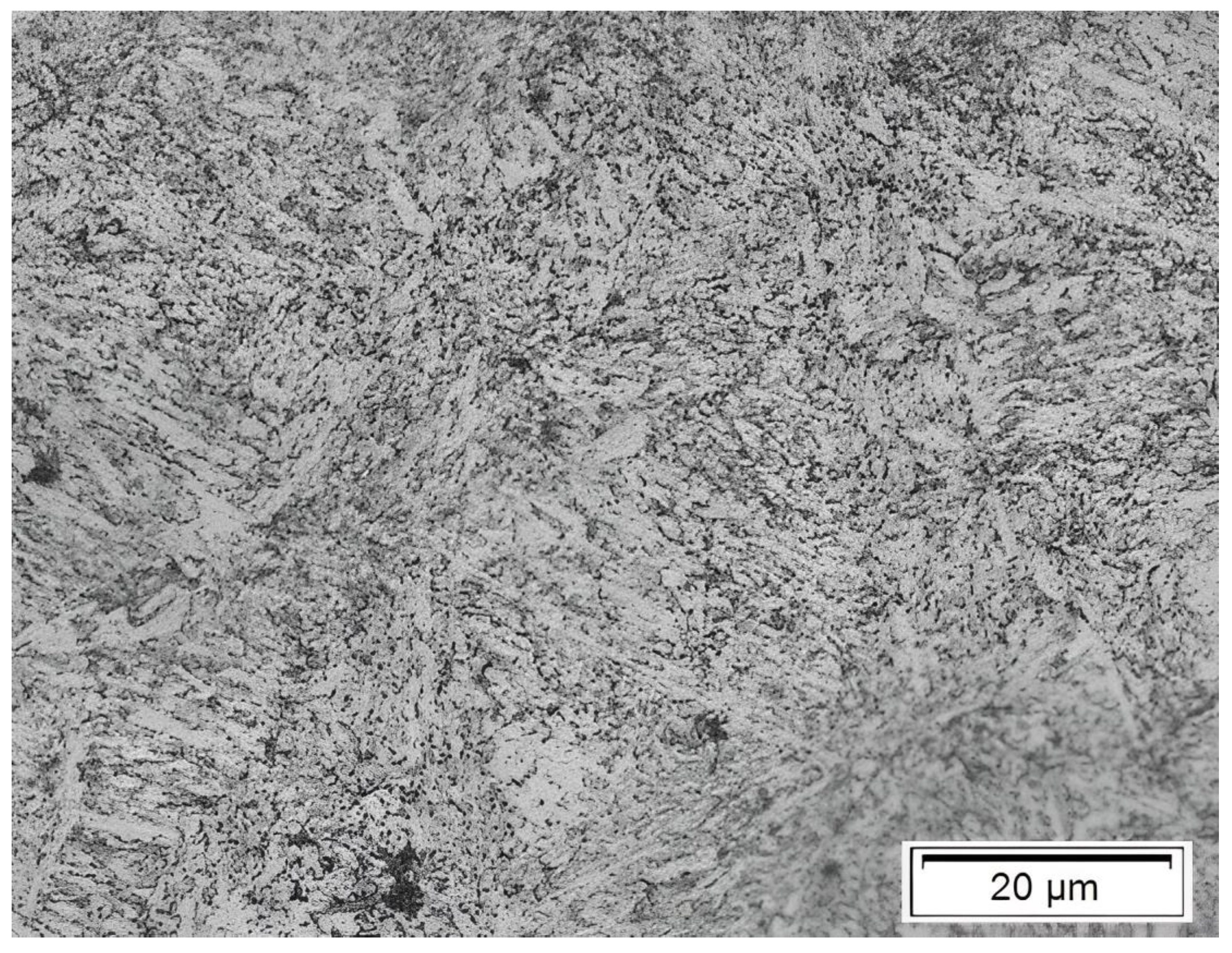
Table 1. Being this steel grade standardised to be quenched at 850 °C (40 min) in an oil bath, and then tempered at 450 °C for 90 min, the 51CrV4 steel (as received) exhibited a tempered martensite microstructure with retained austenite (white phases) [
25,
44] as shown in
Figure 2.
In terms of mechanical strength under monotonic loading conditions, the statistical values were obtained in the proper tests presented in the reference [
25], which followed the ISO 6892-1 [
45] standards as presented in
Table 2. The results refer to a batch of several specimens obtained from different spring leaves in their longitudinal and transverse directions.
Table 2 shows a spring steel with high mechanical strength,
= 1271.48 MPa and
= 1438.5 MPa, but with low (conventional) ductility at fracture,
= 7.53 %. This spring steel grade exhibited a Vickers hardness of 447 HV (corresponding ≈ 45 HRC).
3.2. Fatigue Testing Setup and Specimen Geometry
The spring steel was tested under rotating bending and uniaxial tension/compression conditions for a stress ratio, , of -1 from the high-cycle fatigue regime ( cycles) to the giga-cycle fatigue regime ( cycles). In the HCF region, both rotating bending and uniaxial fatigue tests were carried out at low frequencies, 25 and 150 Hz, respectively, whereas in the giga-cycle fatigue regime, only uniaxial tension/compression tests at a high frequency, 20 kHz were carried out.
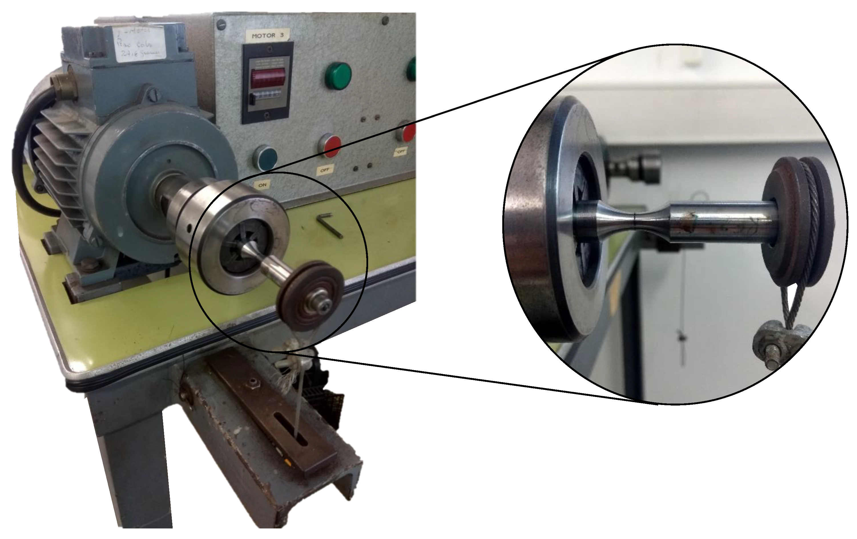
Regarding fatigue tests under rotating bending loading conditions, these were performed with force control under simple bending conditions, with the number of cycles controlled with an automatic counting display. The cyclic force applied on the specimen is induced by a static loading hanging on a bearing and an electric motor operating at 1500 rpm (25 Hz), as illustrated in
Figure 3.
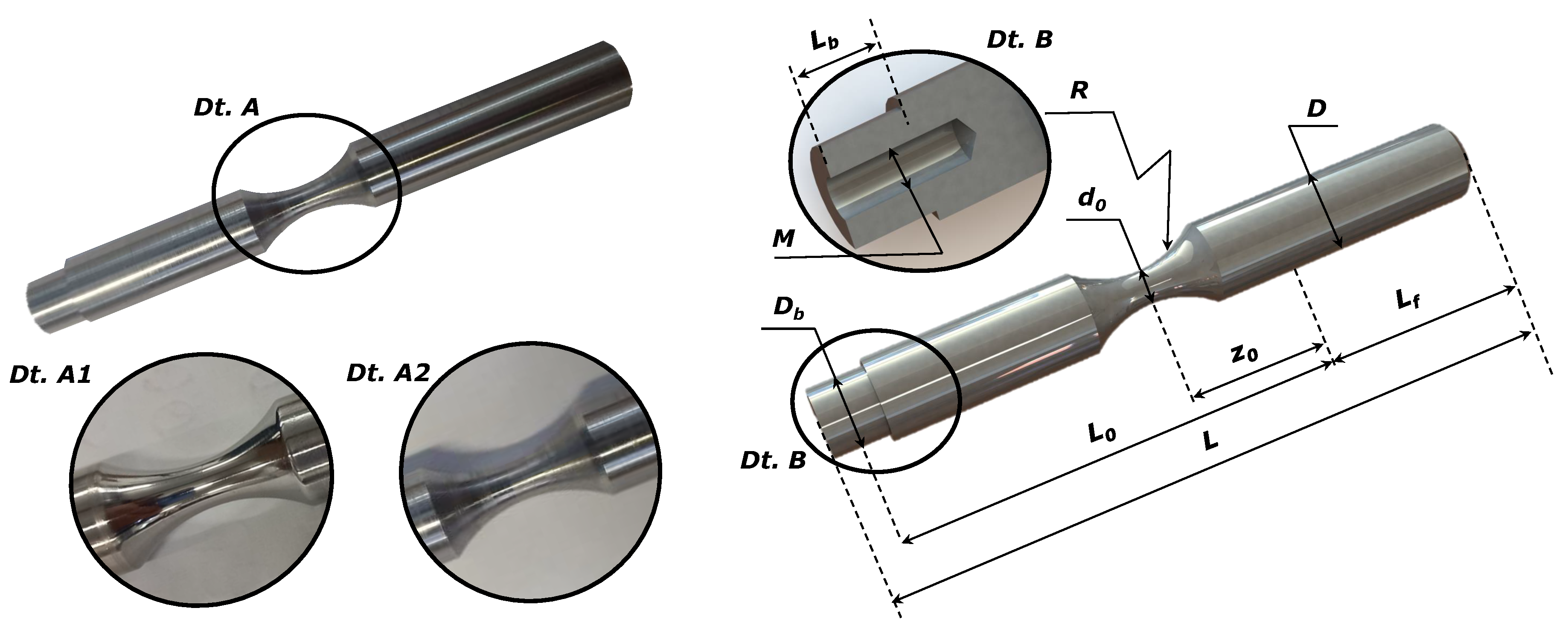
Regarding the specimen geometry for the rotating bending configuration, a hourglass geometry is used with a region for coupling the bearing and a gauge section reduction with radius
R. The specimen geometry complies with the ISO 1143 standard [
46] for rotating bending testing in metallic materials. Furthermore, the value of the radius
R is high enough so that there is no significant stress concentration effect in the analysis zone.
Figure 4 illustrates the smooth fatigue specimen geometry for rotating bending loading showing the finishing detail in the analysis zone.
The details A1 and A2 in
Figure 4 correspond respectively to the surface of a polished specimen and the surface of an unpolished specimen (turned). The smooth specimens were sanded with 800-grit sandpaper, followed by polishing with a diamond cloth of 3
m. On the right side of
Figure 4 the dimensions for defining the specimen geometry are presented.
Table 3 presents the average dimensions of polished and machined smooth specimens used in rotating bending fatigue testing according to ISO 1413 standard [
46].
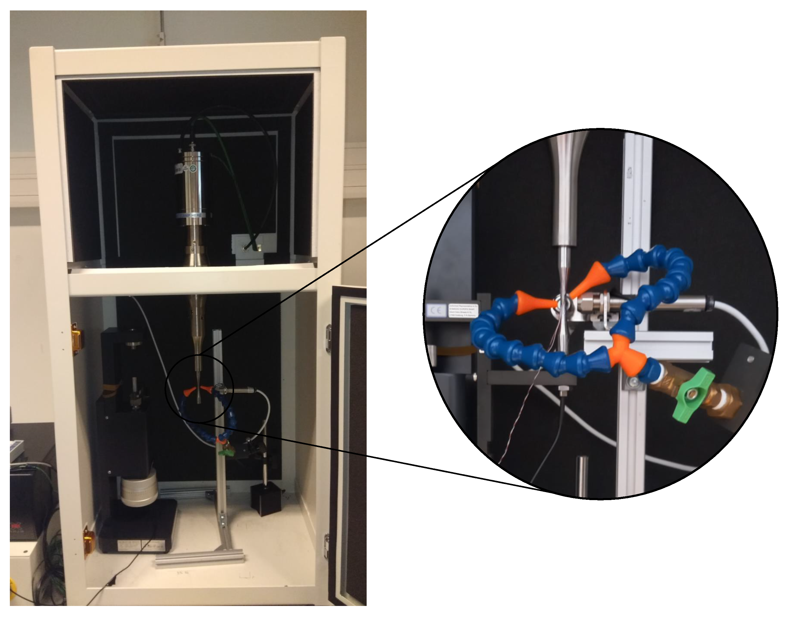
The extension of the fatigue strength curve up to giga-cycle regime is made using the high-frequency uniaxial tension/compression fatigue testing machine, USF-2000 fatigue machine (see
Figure 5) from the Japanese manufacturer Shimadzu, operating at a resonance frequency of 20 kHz under displacement control.
The specimen has an hourglass geometry with a variable cross-section and a test zone being the section with the smallest diameter. Due to the ultrasonic fatigue test operating principle, the specimen must be design to have its 1st longitudinal vibration mode associated frequency in ressonance with the machine excitation one, 20 kHz. Moreover, being the specimen inertial component the equivalent of an external force in a conventional fatigue test, the testing section diameter must be properly choose, in order to achieve the desired stress levels.
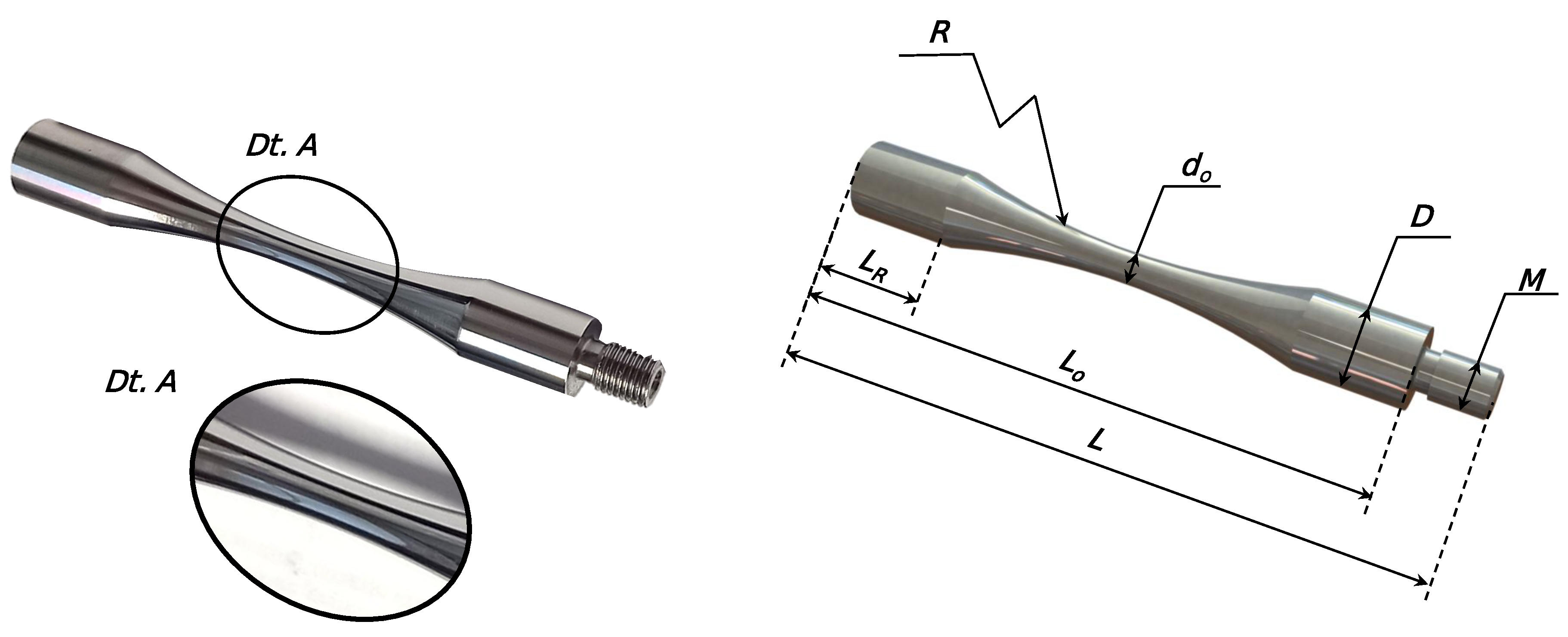
Figure 6 illustrates the geometry of the hourglass fatigue specimen for ultrasonic uniaxial tension/compression testing in the Shimadzu’s machine with the surface finishing in the analysis zone and the CAD model representing the main dimensions for ultrasonic hourglass specimens.
Table 4 summarizes the dimensions considered for the manufacturing of hourglass specimens.
All specimens were tested to verify their natural frequency of vibration, and posteriorly were sanded and polished with 800-grit sandpaper and a 3 m diamond paste, respectively. For the test batch, a random specimen is chosen for dimensional control of the surface roughness (maximum surface roughness allowed, , of 0.1 m and visual control of surface quality using an optical microscope (Olympus SZH).
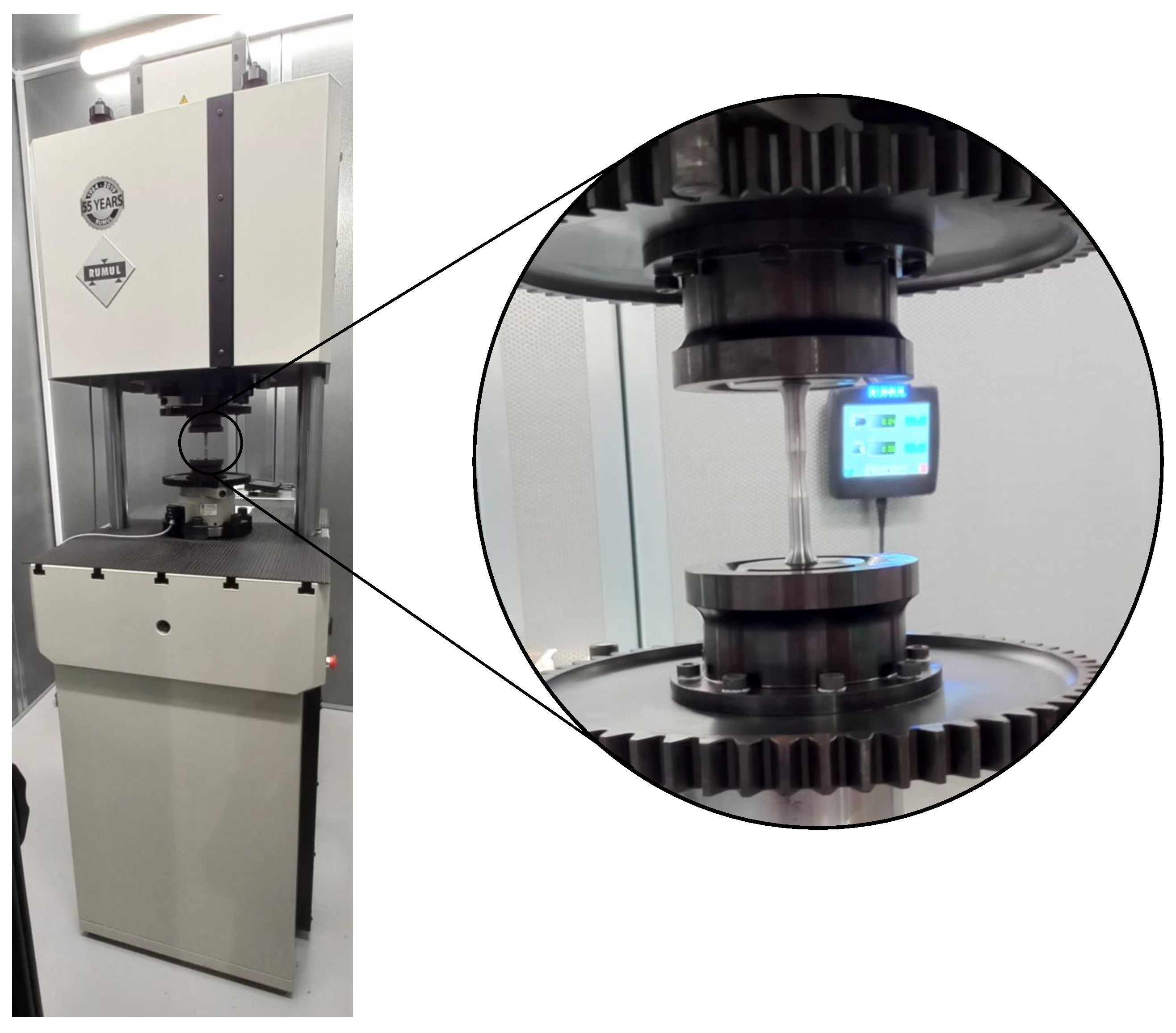
The fully-reversed uniaxial tension/compression fatigue tests at lower frequency (150 Hz which is defined by the controller) are performed using the Rumul Testronic HCF machine operating under load control conditions as illustrated in
Figure 7 [
47,
48]. For measuring the imposed load, a 150 kN load cell is used, which is fitted with built-in acceleration transducers to compensate for the inertial forces resulting from oscillating gripping devices. Data with the number of cycles and applied stress are collected with the help of software and an acquisition system.
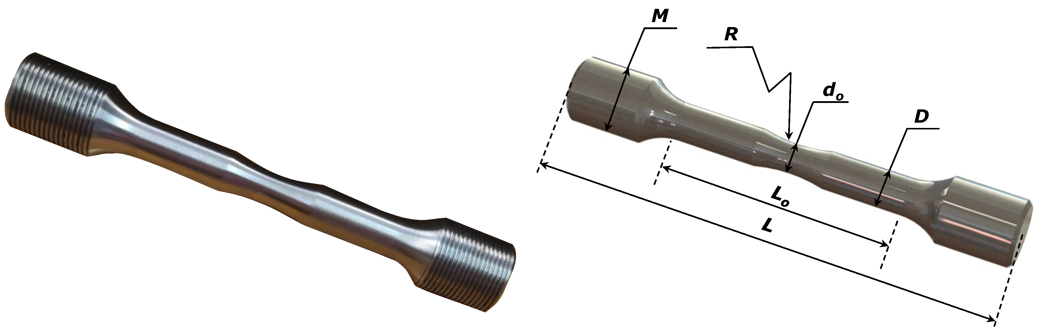
The geometry of the test specimens was developed according to the recommendations of the manufacturer and the fatigue standard [
49] for the standardized grips available (M16×1) and the central geometry of the specimen. The smooth specimens are threaded at both ends, and in the central part the specimens, after machining, were sanded with 800-grit sandpaper and followed by polishing with a diamond paste of 3
m.
Figure 8 presents the hourglass geometry of the test specimen used, with a gauge section reduction zone with radius,
R. The definition of the value for the
R radius is high enough so that there is no significant stress concentration effect in the analysis zone.
Table 5 shows the average dimensions and standard deviations of the analysis region of the specimen.
4. Results and Discussion
In this section, the results of the SN and CFC fatigue curves are presented for rotating bending (25 kHz), tension/compression (150 Hz), and tension/compression at (20kHz) loads. The results are initially presented separately and then subsequently combined to create a full range model from the HCF to VHCF regime for bending and tension/compression, for both SN and CFC models. The effects of frequency and type of loading on fatigue strength are analysed and discussed. The fatigue fracture surfaces obtained by SEM and EDS analysis are considered to clarify the results obtained.
4.1. Basquin SN Fatigue Model
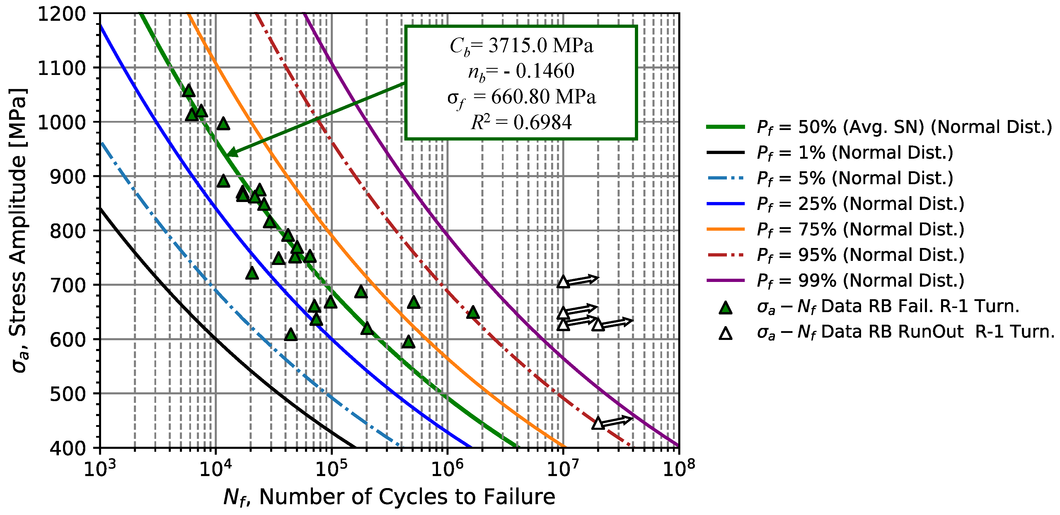
The rotating bending fatigue tests were carried out from a level stress amplitude,
, close to the yield strength of the material, up to a stress amplitude where run-outs begin appearing, corresponding to a fatigue life around of 10
7 cycles.
Table 6 summarizes the parameters
and
obtained by the linear regression model, for specimens with different surface finishing conditions. According to the results presented in
Table 6 and
Figure 9, a value of
equal -0.1460 and a value of
equal 3715.0 MPa with a coefficient of determination of
were obtained. However, considering only polished specimens, the value of
increases to -0.082, and
decreases to 2005.68 MPa, as expected for specimens tested in the HFC regime with a better surface quality. The change of the exponent
was due to the most extreme point that fractured in the zone close to the occurrence of run-outs, as can be seen in
Figure 10, which hence increases
and decreases
. In addition, from the comparison between the data set corresponding to the turned and polished specimens, one verified that specimens with a surface roughness of 0.5
m had no significant influence on the fatigue strength.
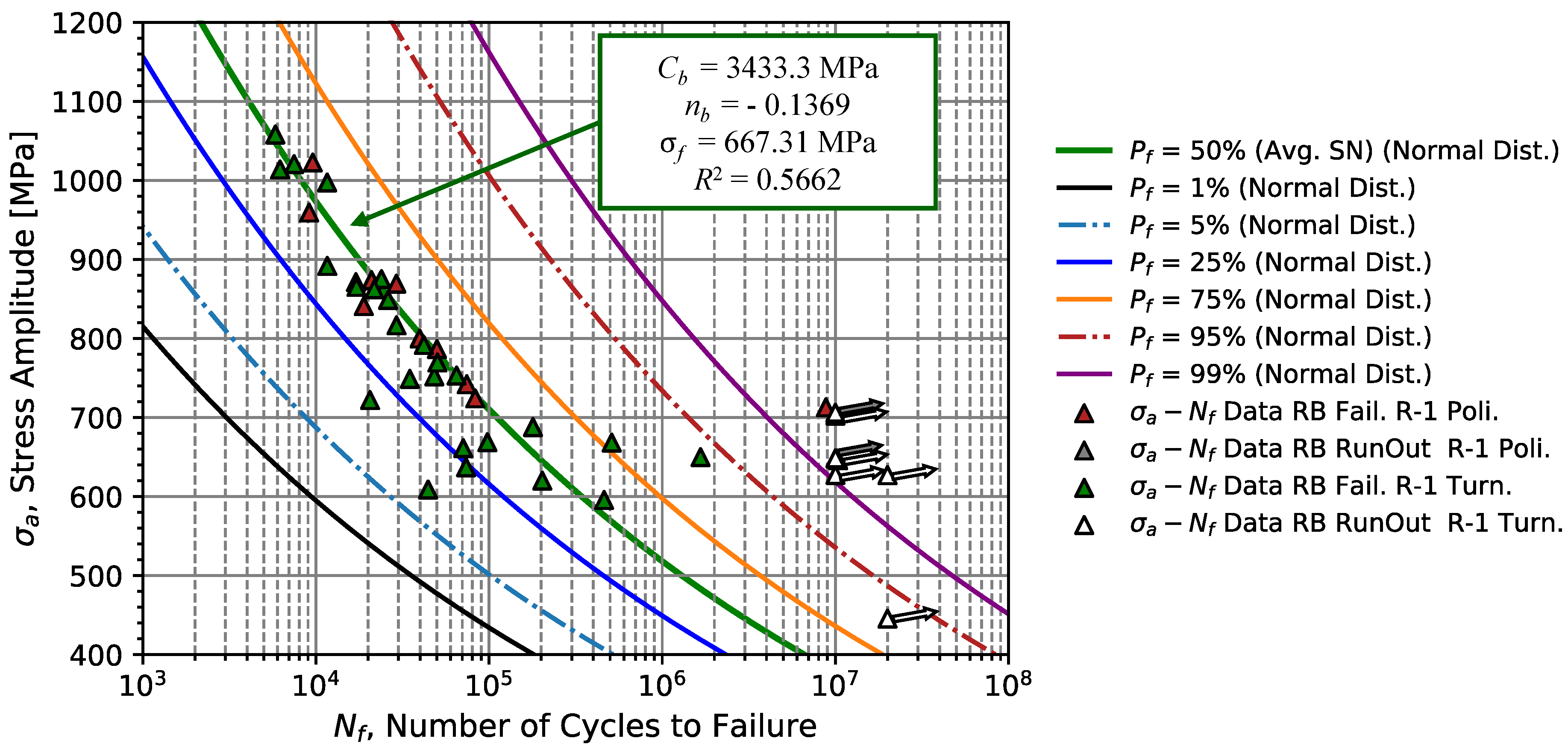
Thus, considering a combination of the obtained results from turned and polished specimens, one verifies that
and
are close to the SN fatigue model considering only turned specimens, such that the combined model results in
= -0.1369 and
= 3433.3 MPa with a coefficient of determination of
of approximately 0.57. Additionally, the fatigue limit,
, does not undergo significant changes, 660.8 MPa for specimens only turned and 667.3 MPa for specimens turned and polished. The fatigue limit is determined by the arithmetic average of the data set below the stress amplitude level in which the first run-out was observed. Notice that this value of fatigue limit is 1.48 of the Vickers hardness value, which corresponds approximately to the relationship of
[
6]. The low calculated values of
are associated with the high scatter obtained in the zone close to the fatigue limit stress. The parameters obtained for the equation model (
1) consider that the distribution of the points around the mean curve is given by a Gaussian distribution, and hence the outliers increase significantly the scatter of the model.
Regarding the failure probability curves (Equation (
3)) in
Figure 10 obtained from
Table 6, it is verified that the median curve contains most of the failure points for stress amplitudes higher than 700 MPa. In the range of 600 and 800 MPa, it is verified that some failures occur for a failure probability inferior to 25 %. Moving on to the analysis in longer lives, the statistical model cannot contemplate the outliers correctly, as is the case of the polished specimen fractured close to 10
7 cycles.
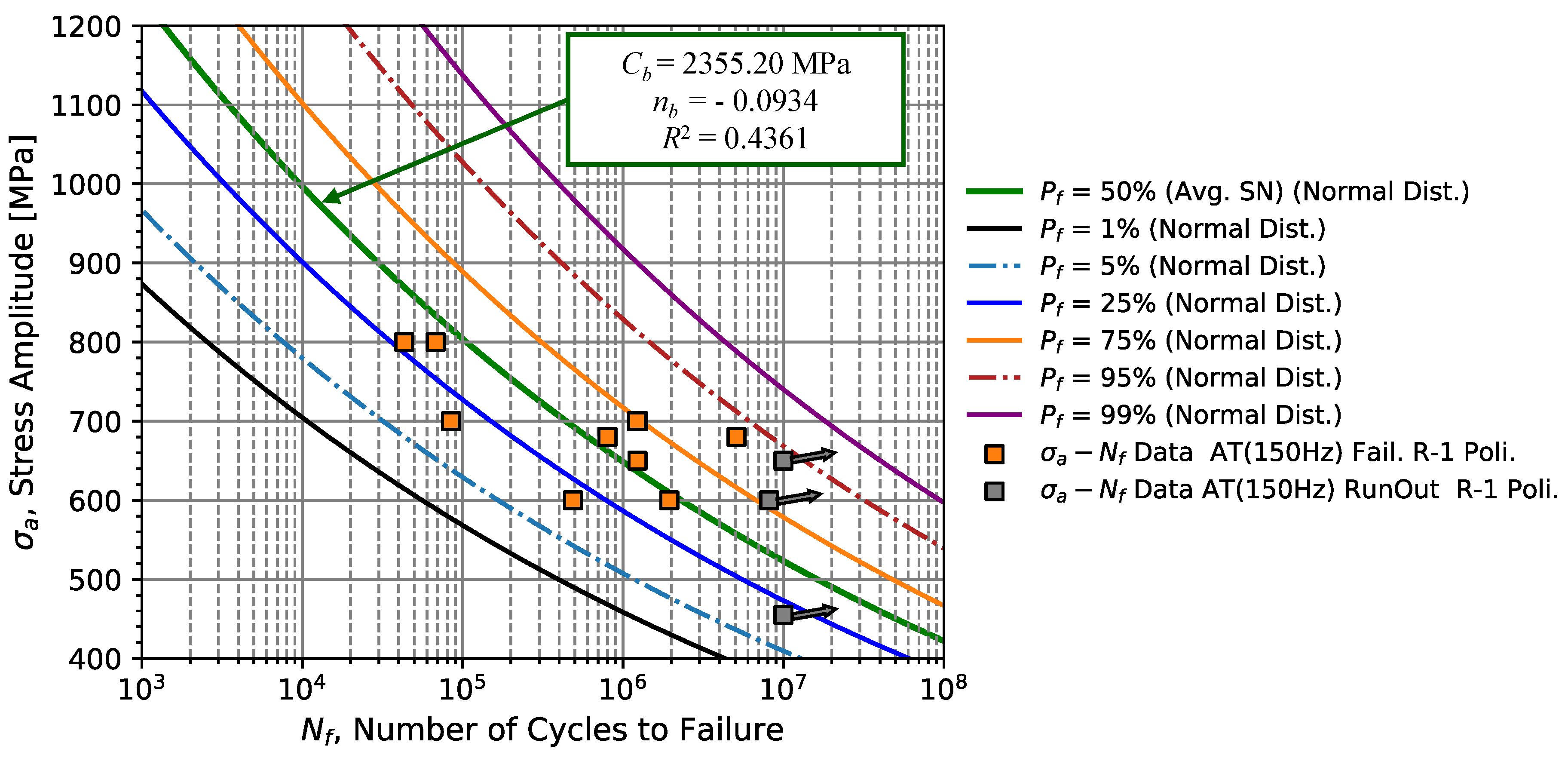
Regarding the tests carried out under fully-reversed stress conditions at subsonic frequency (150 Hz), for a region of interest from
to 1.0
cycles, a reduction in the resistance coefficient value,
, to 2355 MPa is obtained when compared with results obtained for cyclic rotating bending conditions. The value associated with the regression resistance exponent,
, also decreases slightly to values around -0.09. The coefficient of determination of
= 0.4361 indicates a large variance of the results in relation to the linearised regression model. In fact, from
Figure 11 it is clear that for stress amplitudes below 700 MPa, we will be in the fatigue limit zone and the occurrence of outliers is likely increasing. Under these conditions, regressive models considering distributions based on the outer limits are recommended.
Table 7 summarizes the coefficients of Basquin’s model (equation (
1)).
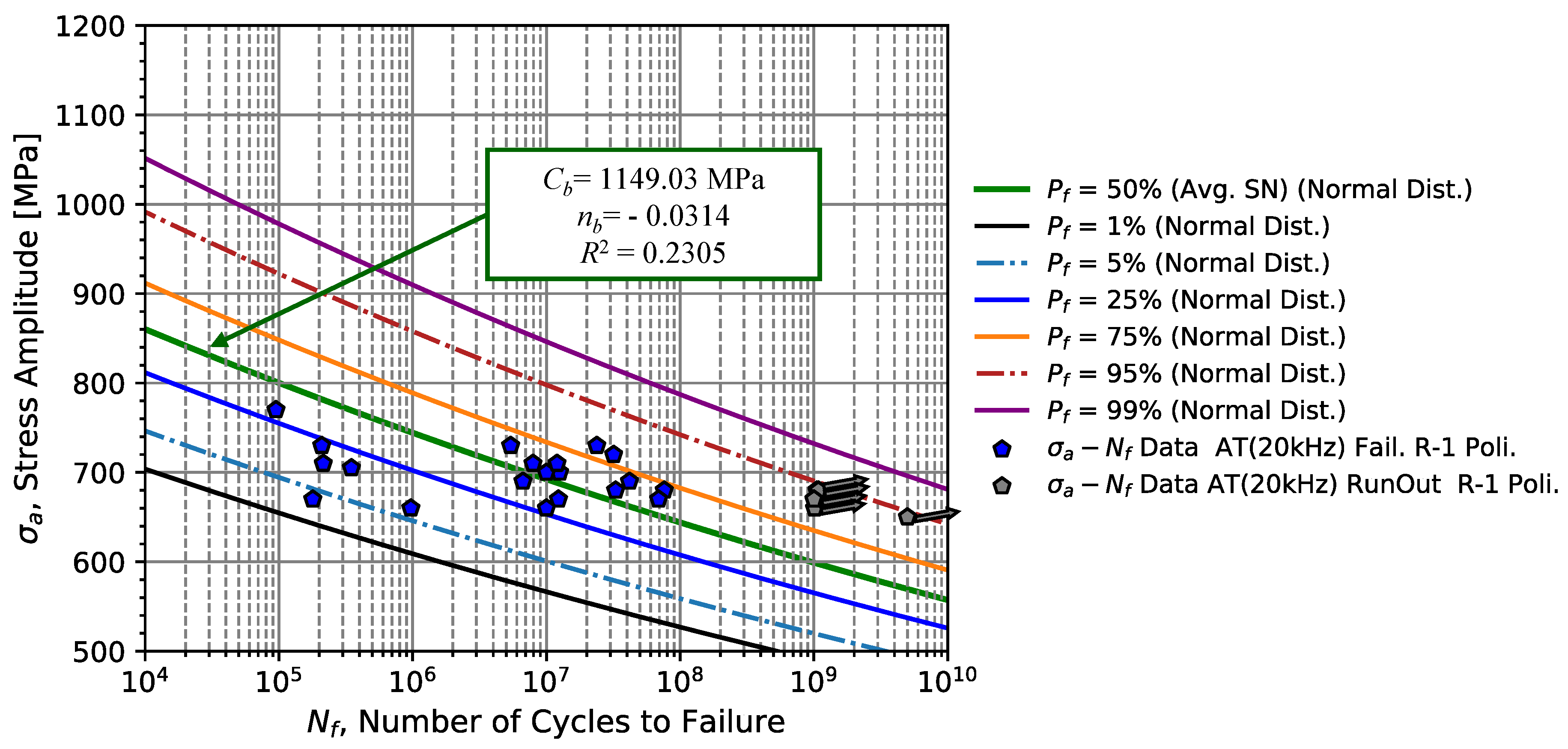
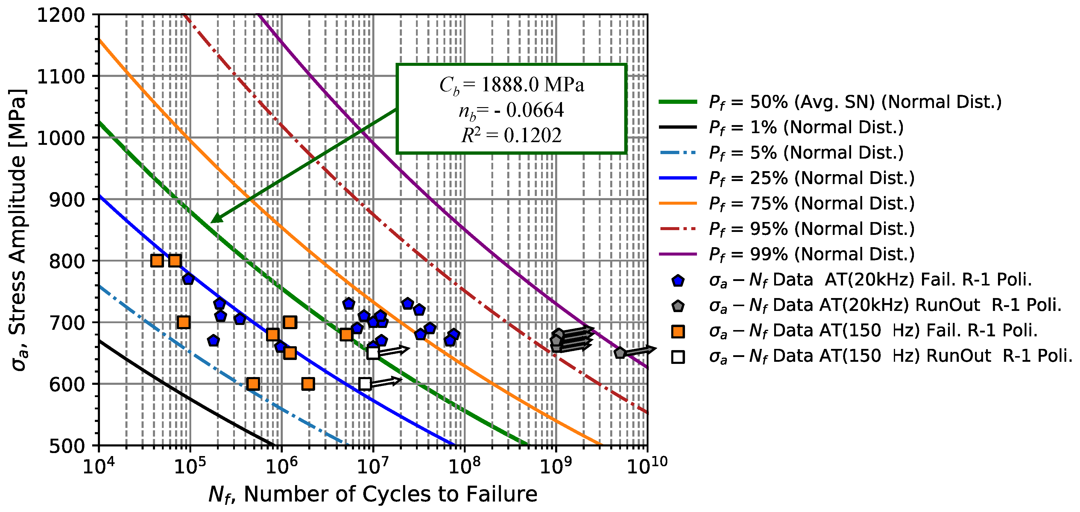
Increasing the testing frequency to 20 kHz, it is possible to test the spring steel up to 1.0
cycles in a suitable testing time. Analysing the region of interest from 1.0
to 1.0
cycles as shown in
Figure 12, it is verified an increase in the fatigue life scatter of the spring steel for the same stress amplitude. From the regression analysis, the resistance coefficient,
, decreases to half of the value for tension/compression conditions at subsonic frequencies, while the resistance exponent,
, is reduced to one-third of the previously obtained value. Following the same trend, the value of the coefficient of determination also decreases by half to
= 0.2377. This analysis sequence indicates that the regression model is practically not adequate in this analysis region due to the high scatter of the data and the increase of run-outs obtained.
Table 7 summarizes the quantities of Basquin’s model (Equation (
1)) and the respective statistical parameters of the regression.
Since the frequency effect affects the fatigue strength, the frequency sensitivity of spring steel is analysed using the data set presented in
Figure 11 and
Figure 12, 150 Hz and 20 kHz, respectively. Since both data are overlapped, one concludes that the spring steel 51CrV4 has a low sensitivity up to 20 kHz, for the fatigue life region between 1.
to 1
cycles. Quantitatively, the frequency effect can be evaluated by determining the nominal stress,
which does not take into account the frequency effect, and it is given as
where the effective stress,
, is the stress that takes into account the frequency effect, and the correction factor
, that is the ratio,
with
and
denoting respectively the Young’s modulus evaluated for quasi-static conditions and the Young’s modulus evaluated with the existence of frequency effect. For spring steel 51CrV4, the factor
is approximately 0.98, which indicates that there is only a 2 % variation of Young’s modulus when we excite the material at a frequency of 20 kHz. Thus, converting the effective stresses,
, presented in the data of
Figure 12 by the Equation (
6) the stresses are slightly reduced as presented in
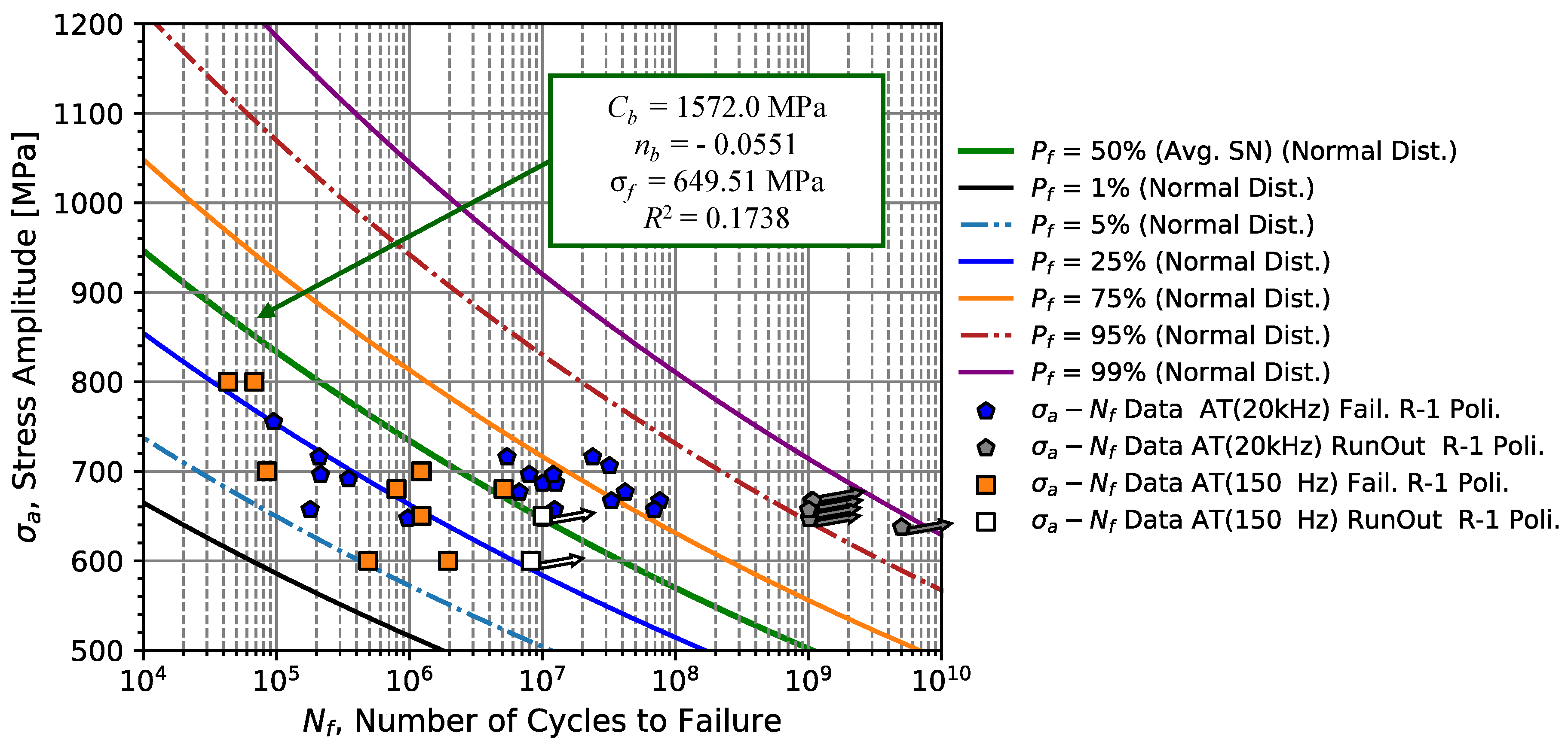
Figure 14. From the analysis performed to identify the fatigue limit of 51CrV4 steel under tension/compression conditions, results in
MPa. In similarity to the bending conditions, the fatigue limit is very close to the relationship of
[
6], such that the ratio between
and HV is 1.45.
In is important to note that by applying this correction to the data tested at 20 kHz, the coefficient of determination increased from 0.1202 to 0.1738, also verifying a greater overlapping of the fatigue failure data for stresses between 650 and 700 MPa. Furthermore, for a stress of 650 MPa, one verifies that the first run-out obtained for tests at 150 Hz is almost coincident with the run-out at the lowest stress obtained for 20 kHz. Regarding the resistance parameters, the coefficient
decreased from 1888 to 1572 MPa while the exponent,
, underwent a slight change, changing from -0.0664 to -0.0551.
Table 8 presents the summary of the statistical parameters obtained for each of the regressions.
4.2. CFC Fatigue Model
Although the Basquin SN linear regression model has shown to predict material failure for higher stress amplitudes, that model does not allow a good fitting of the failure probability to low-stress levels. Additionally, the SN model does not take into account the outliers and run-outs in its predictions. To overcome these constraints, the CFC fatigue model using a 3-parameter Weibull distribution is considered.
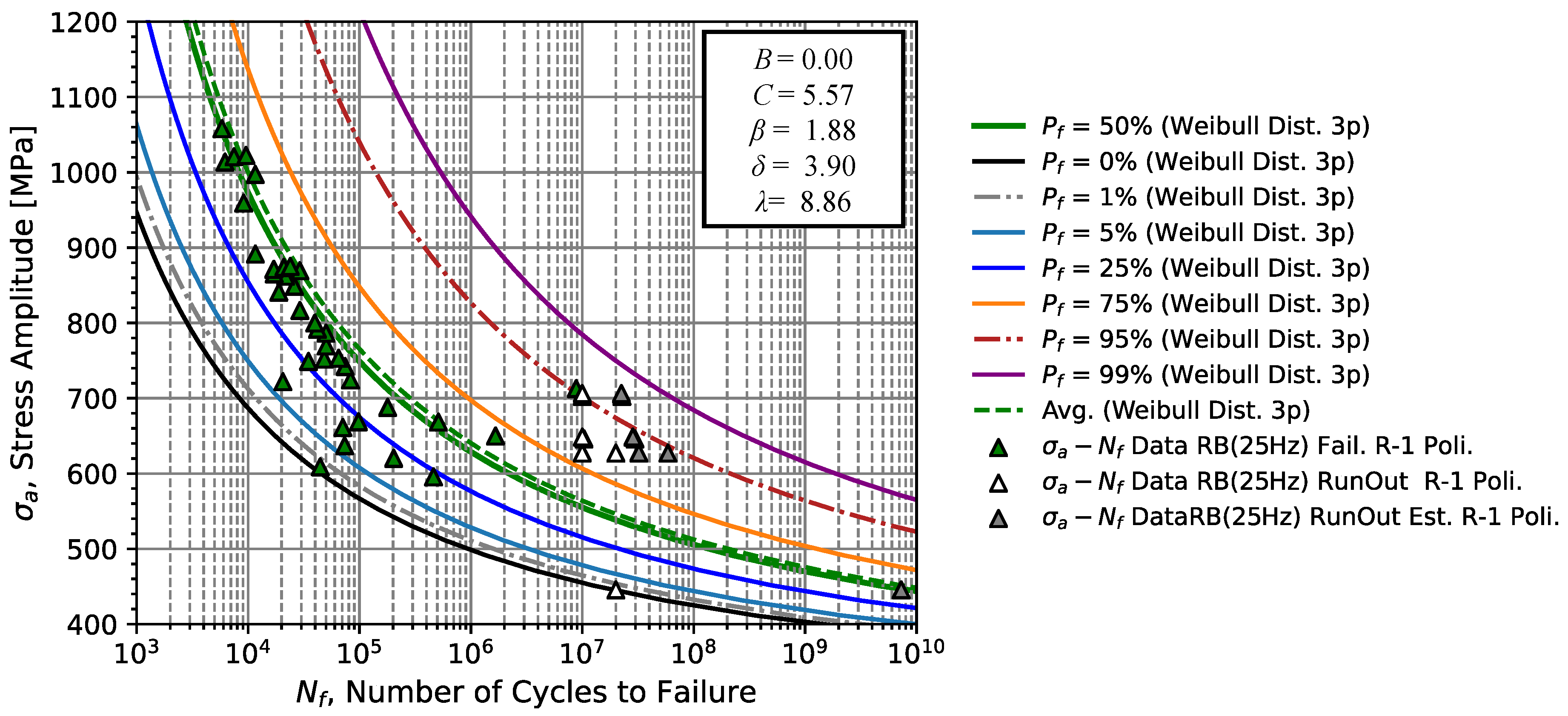
Figure 15 presents the failure data of smooth fatigue specimens under rotating bending loading conditions in a stress field given by the CFC fatigue model. The estimators determined for the construction of the SN-field presented in
Figure 15 are presented in
Table 9 column 1. According to the results obtained by the estimation methods, a fatigue limit value of 261.0 MPa is estimated for a scale parameter,
, shape parameter,
, and the location parameter
.
Figure 15 shows that the mean curve of the Weibull distribution and the corresponding median curve are very close to the values for the normalized random variable,
v of 12.32 and 12.07, respectively. This proximity indicates that the determined distribution is almost symmetrical with the largest amount of data occurring between the 25th and 75th percentiles % for loads greater than 700 MPa. Concerning stresses lower than or equal to 700 MPa, it appears that the model allows including run-outs up to a failure probability of 99 %. Note that only one of the data points occurs for a failure probability of less than 1 %.
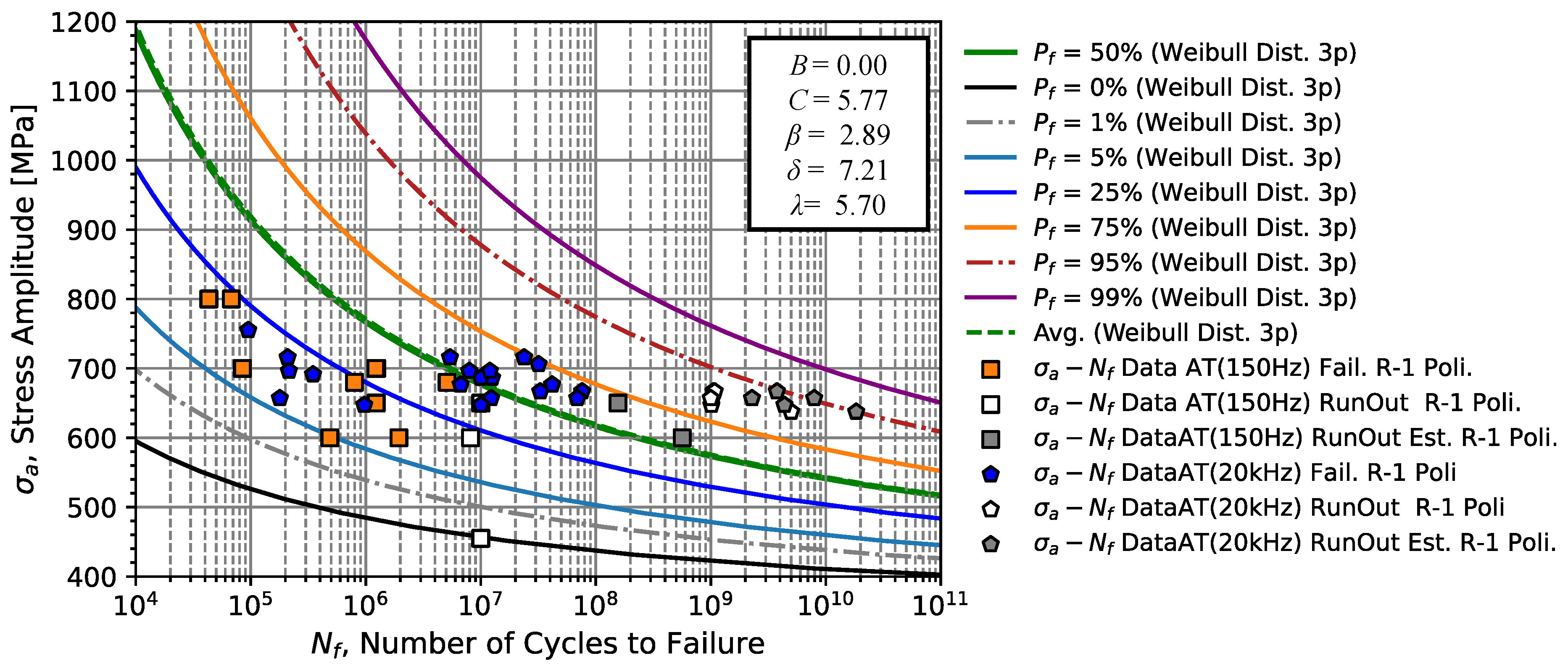
For subsonic and ultrasonic tension/compression fatigue tests, percentile curves illustrated in
Figure 16 were constructed considering the parameters presented in
Table 9 column 2 (considering both failures and run-outs). Notice that the estimate for the 450 MPa run-out that was tested to a life of 10
7 cycles is nearly 10
10 cycles.
According to these obtained results obtained, a fatigue limit value,
C, for the axial tension/compression loading of 319.1 MPa is estimated, which is a higher value, around 22.60 % when compared to the value of
C = 261 MPa for the rotating bending model (see
Figure 15). With respect to the distribution parameters, this model obtained a shape parameter,
of 2.89, a scale parameter,
of 7.21, and a location parameter
of 5.70. Since the
parameter shapes the probability density function, it is expected that for more dispersed data along the SN field, the value of
will be higher. However, these parameters refer to the random variable
V and therefore only the combination of the applied stress, number of cycles and parameters
B and
C can explain this change in values in greater detail. Analysing the failure occurrence zone in more detail, one can observe from
Figure 15 that the mean curve of the distribution and the percentile corresponding to the median are even closer with the greater amount of data occurring between the 5-95 % percentiles.
4.3. Combined Fatigue Model
The combined fatigue model requires that the data sets considered are provided for the same test frequency and type of loading. Regarding the frequency effect, this has already been analysed previously, and no significant influence on fatigue resistance was observed for 20 kHz. With respect to the effect of the type of loading, it is seen in
Table 8 that a higher fatigue strength in the finite life zone when subjected to bending loads. This conclusion is consistent with some previously conducted studies [
50,
51] and engineering design literature [
52] that compare this detrimental effect of axial stress versus bending. In addition, it is also verified that this harmful effect will tend to be greater for lower life regimes.
Despite the differences in fatigue strength for the two types of loads, it is verified that for lower stress amplitudes, there is an overlap of strength data under rotating bending and axial tension/compression stresses. Assuming that in the zone close to the fatigue limit, the loading effect for 51CrV4 steel can be neglected since the fatigue limit for both loading conditions is very close with an average value of 655.16 MPa, and an SN curve is determined containing these data sets.
Figure 17 presents the SN curve and the curves corresponding to the percentiles of the Gaussian function obtained from the experimental data.
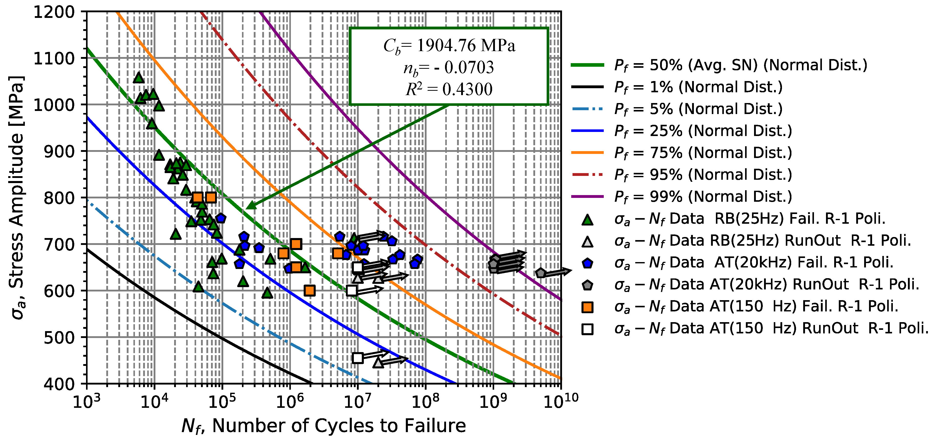
Comparing
Figure 17 with
Figure 10 and
Figure 14, it can be observed that there is a certain deviation in the gradient of the SN curve compared to resistance data between the range of 600 and 900 MPa. The obtained SN curve regression parameters were
= 1904 MPa and
= -0.0703 with a
of 0.43. These values are close to those obtained for the SN curves in tension/compression uniform stress, showing the large weight that failure data in the fatigue limit region have on the parameters of the average SN curve.
Table 8- column 3, presents the data used to create the percentile curves of
Figure 17. According to the results obtained, the SN curve with stress amplitude, will not be the most suitable for representing the combined fatigue prediction model of 51CrV4 steel.
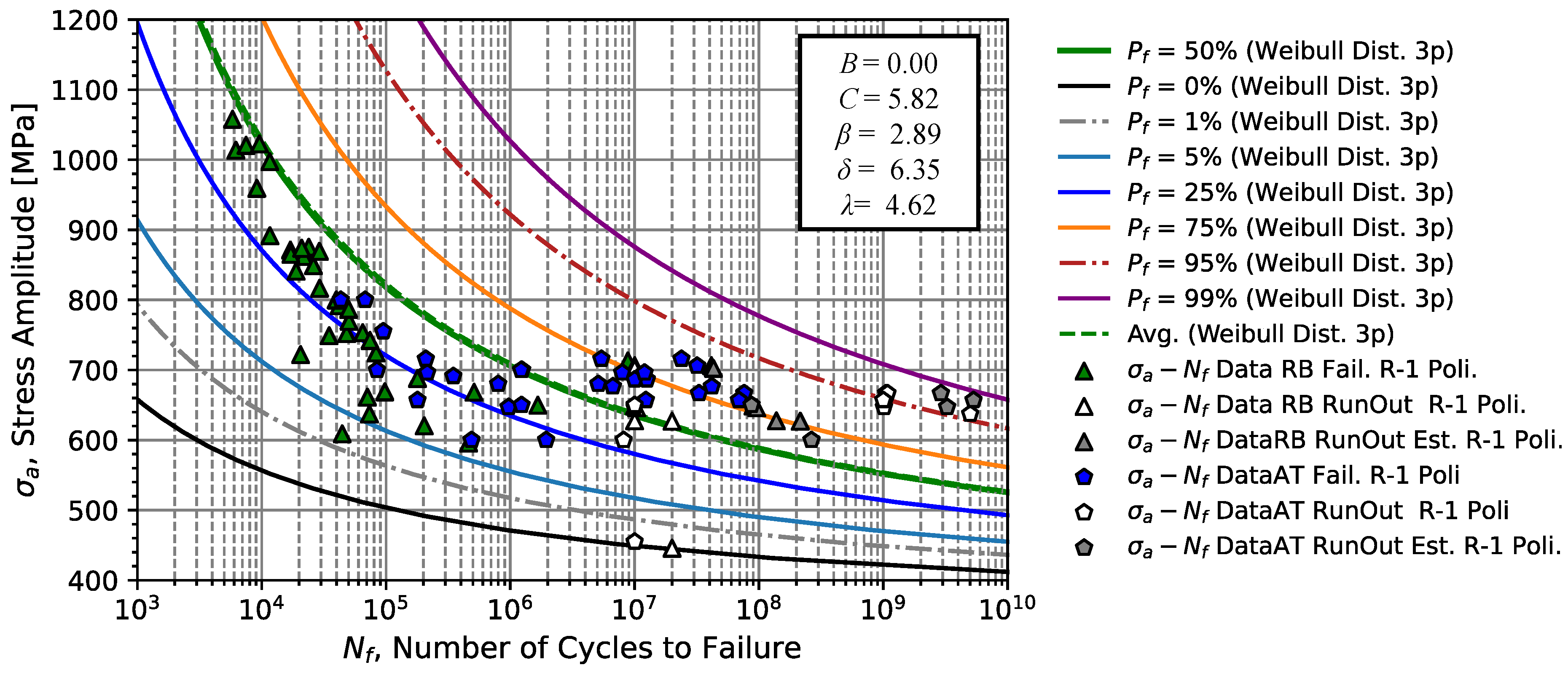
Considering the advantages of fitting the CFC model (already shown) on the test data set, the CFC model is now analyzed. For the CFC model with the normalized random variable
V, the joint data of rotating bending and compressive stress/strain alternation were used. The parameters calculated and used to build the CFC model in
Figure 18 are presented in
Table 9-column 3. It should be noted that the introduction of information regarding higher stress amplitudes, in this case, due to fatigue data from rotating bending, allowed the estimated fatigue limit to be changed to 338.4 MPa. However, this increase was only 6.05 %, which indicates that the information obtained by the axial alternating tensile tests has a great impact on the estimation of the fatigue limit of the model. Furthermore, this impact is verified in the scale parameter
which remained at 2.89. Regarding the rest of the parameters, a shape parameter
of 6.35, and a location parameter
= 4.62 were computed. Concerning the percentile curves, again values are very close to the mean curve and median curve, (
v = 10.28 and
v = 10.21, respectively). Furthermore, it is also shown in
Figure 18 that the data set under analysis is all contained in the probabilistic band corresponding to the failure probability of 1 and 99 %.
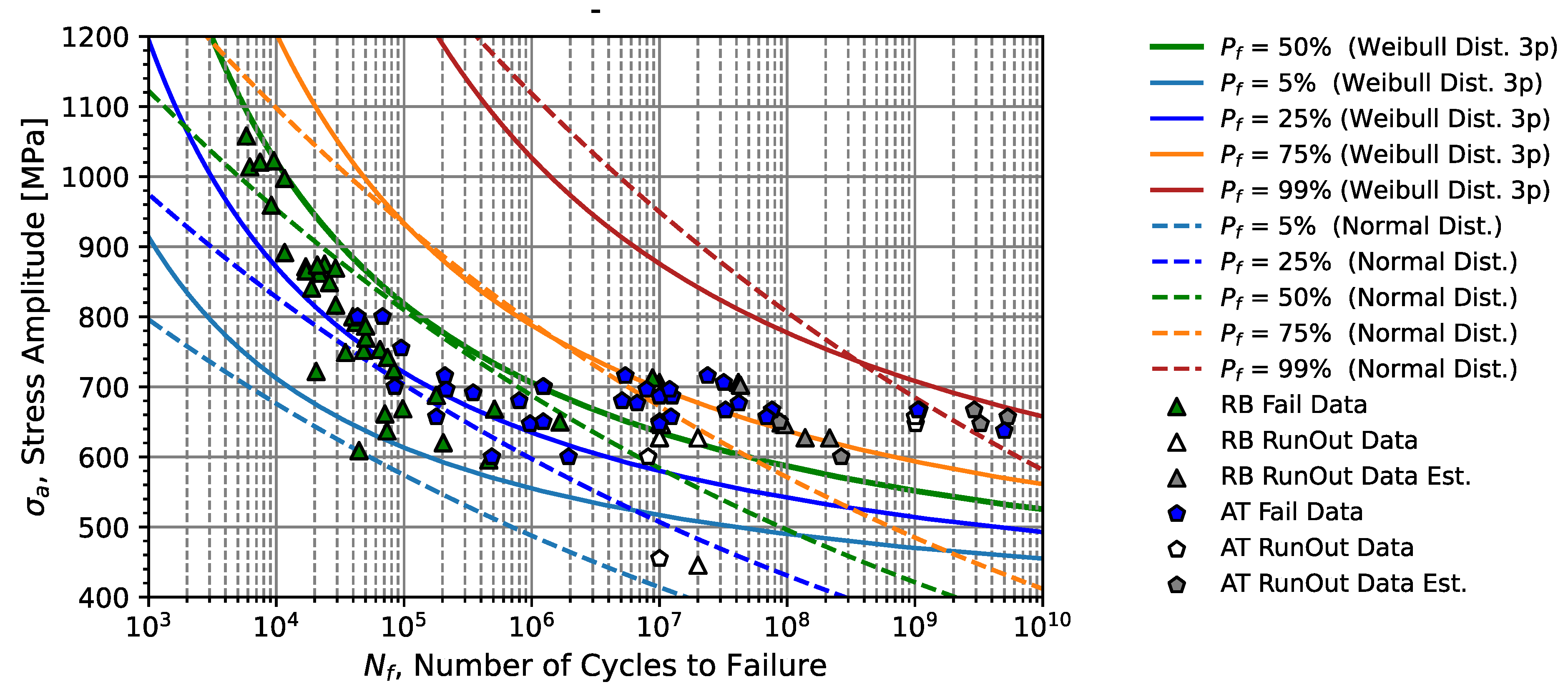
Thus, from the comparison between the SN and CFC fatigue prediction models, some comparative points can be mentioned. According to
Figure 19, in addition to the fact that the SN model is monotonically decreasing until it vanishes, while the CFC model tends to its limited value
. The percentage curves appear that the median curves and the 25th and 75th percentage curves tend to coincide in the intermediate zone of the analysed data, approximately around 800 MPa, becoming divergent for higher and lower stresses. Another big difference is that the percentile curves obtained by the SN model tend to be conservative for higher stress amplitudes. Furthermore, for long lifetimes, the SN law tends to be non-conservative since it does not consider the effect of run-outs on the SN field estimate. In summary, the CFC model produces a better fatigue strength prediction for both high-cycle and giga-cycle fatigue regimes, and this model is recommended for future predictions.
With respect to specimens tested under fatigue tension/compression loadings, in this region of interest, most fractures occurred due to the initiation of cracks on the surface, except in one case. In this single case, the crack started through a non-metallic inclusion in the interior zone of the specimen. Concerning the tests carried out at a stress of 600 and 700 MPa, the specimens that obtained a life of 5
and 8
cycles, respectively, failed from a "macro" surface scratch contrary to the rest of the specimens. Under these conditions, the probabilistic model given by the normal distribution considering the parameters presented in the
Table 7 subsonic tensile column, encompassed all the test specimens that failed in a failure probability between 5 and 95 %.
4.4. Fracture Surfaces Analysis
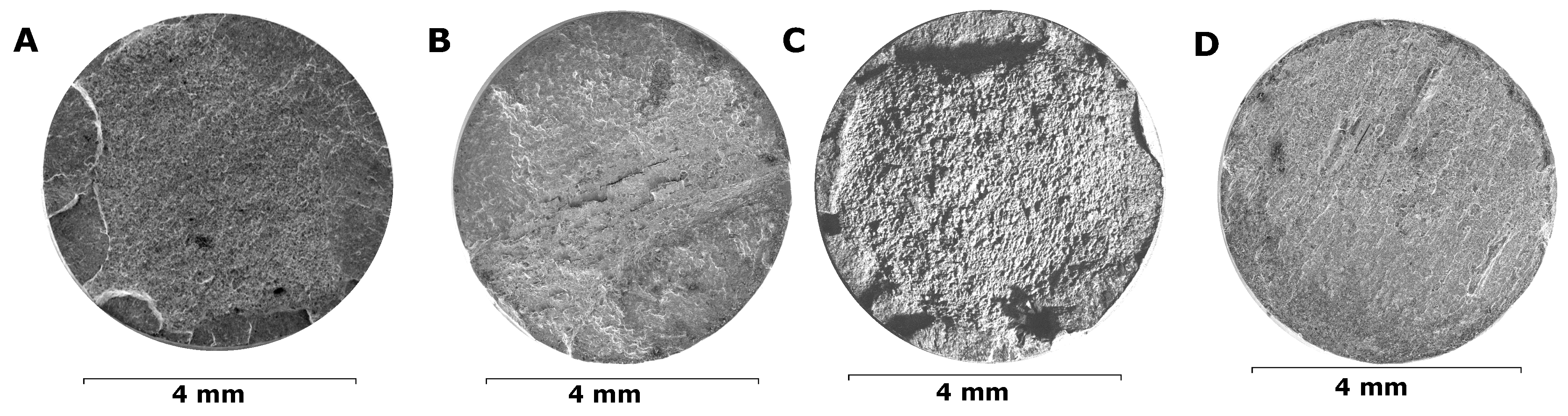
Fracture surfaces analysed via SEM for rotating bending specimens (for three distinct applied stress amplitude levels) are illustrated in
Figure 20.
Figure 20A,B are associated with the highest stress amplitude region. It is clear that there is an initiation of multiple cracks around the specimen circumference with crack propagation areas of 6.20 and 7.33 mm
2 and a critical crack length of 0.84 and 0.95 mm, respectively. Some of these cracks along their propagation process merge with other cracks in their vicinity. Additionally, it is visible that some of these cracks produced larger cracks than others. Reducing the load to 816.56 MPa, the occurrence of multiple initiation cracks with different crack lengths is still verified. In this condition, a total crack area of 12.99 mm
2 and a critical crack length of 1.671 mm are measured. In the lowest loaded region (595.67 MPa), the failure mode predominantly occurs by single crack initiation, which propagates to an extent of almost half the specimen diameter as shown in
Figure 20D with 5.07 mm
2 and a length of 1.847 mm.
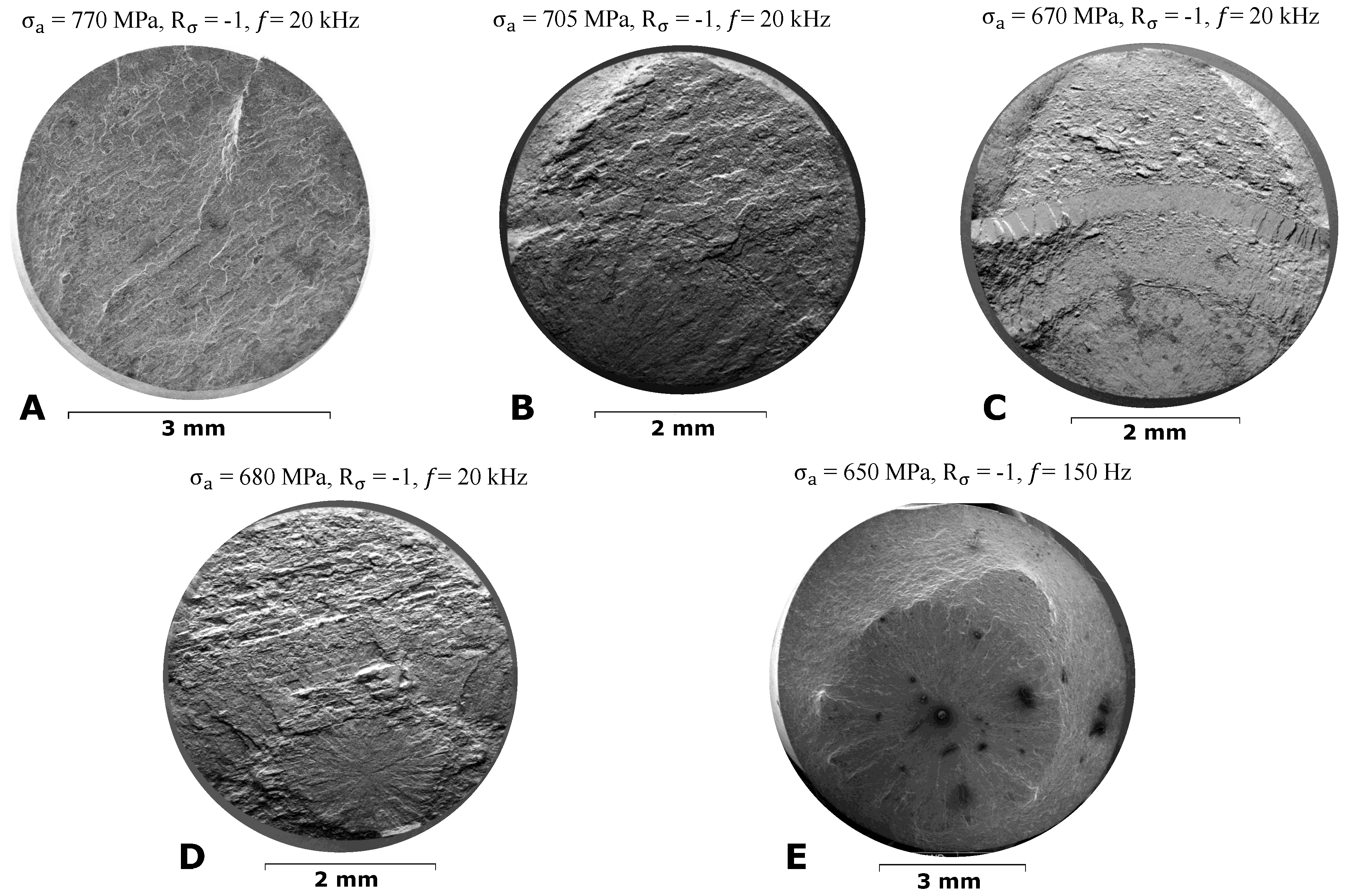
With respect to specimens tested under fatigue tension/compression loading,
Figure 21 presents the comparison of fracture surfaces for different stress amplitudes of specimens tested at 150 Hz and 20 kHz. One verifies that for higher stresses between 770 and 705 MPa (
Figure 21A and B, respectively), the failure mode occurs mainly by crack initiation on the surface. However, for stress amplitudes below 680 and 670 MPa, a mixed failure mode occurs. Therefore, under these load conditions, crack initiation can occur either on the surface or from in the interior or sub-regions of the specimen from non-metallic inclusions. The occurrence of both situations will depend on several factors such as surface roughness, and inclusion size, among others. In
Figure 21D,E the occurrence of failure with crack initiation in the core of the specimen is verified. While the fracture surface of
Figure 21D exhibits an inclusion with a shallow and elongated shape, the inclusion in the fracture surface of
Figure 21E, has a circular shape.
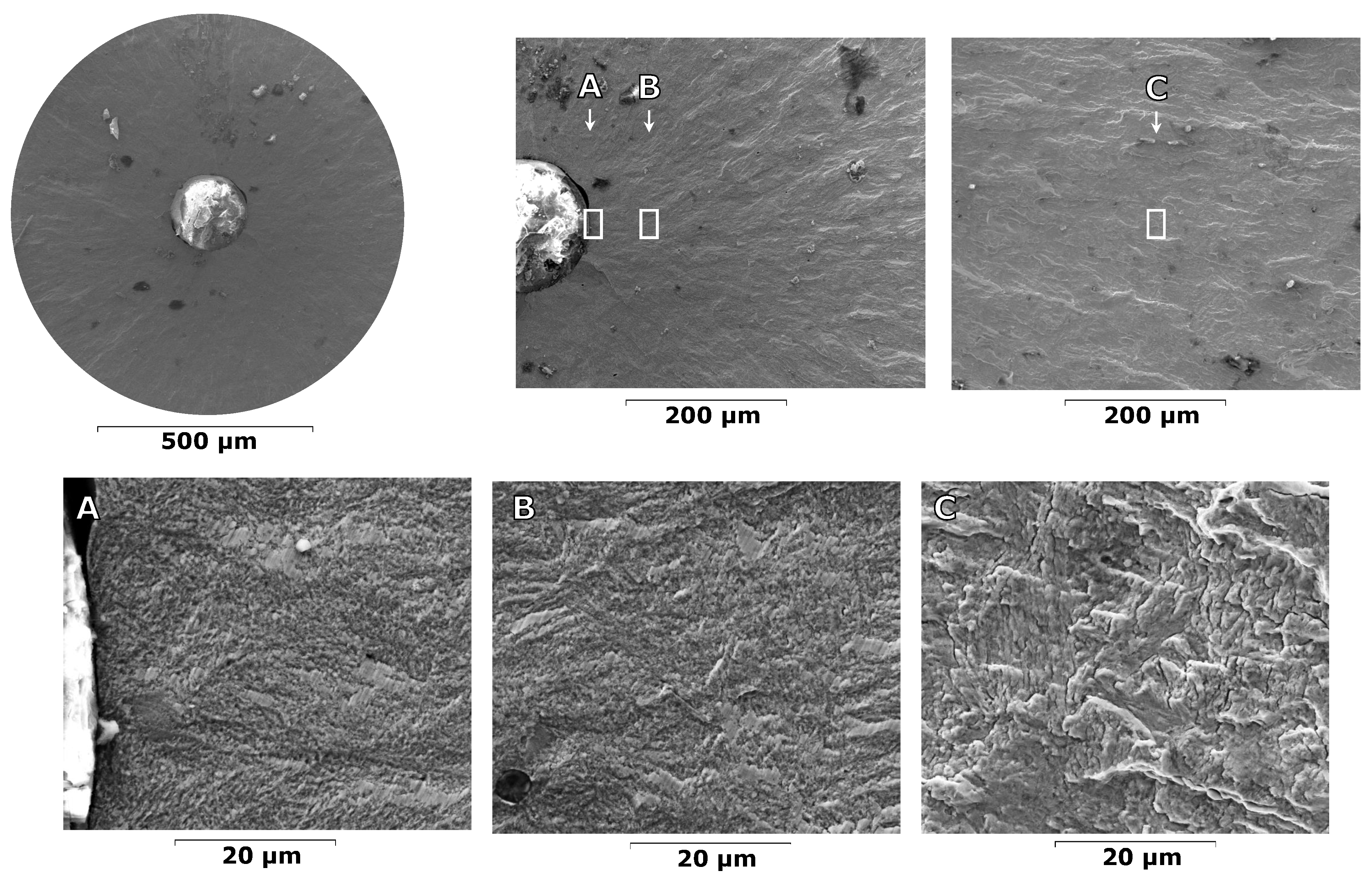
A more detailed analysis of the fracture surface of
Figure 21D is performed in terms of surface morphology around the non-metallic inclusion.
Figure 22 shows the fracture surface of the fish-eye with details on the morphology in the zones close to the inclusion. Comparing zones A and B (immediately after the inclusion) with zone C (away from the inclusion), the surface roughness is very different. Zone C shows higher roughness than zones A and B. From this verification, it is possible to conclude that the initiation occurs without the formation of a fine-granual-area zone (FGA) [
6]. From the analysis of zone C, fracture micro-mechanisms predominantly by cleavage are visible.
In this region, surface defects become very important for the occurrence of failures or run-outs. As observed for specimens tested under subsonic fatigue conditions (150 Hz) in tension/compression, some failures occurred on the free surface of the specimen or from non-metallic inclusions in the interior of the specimens.
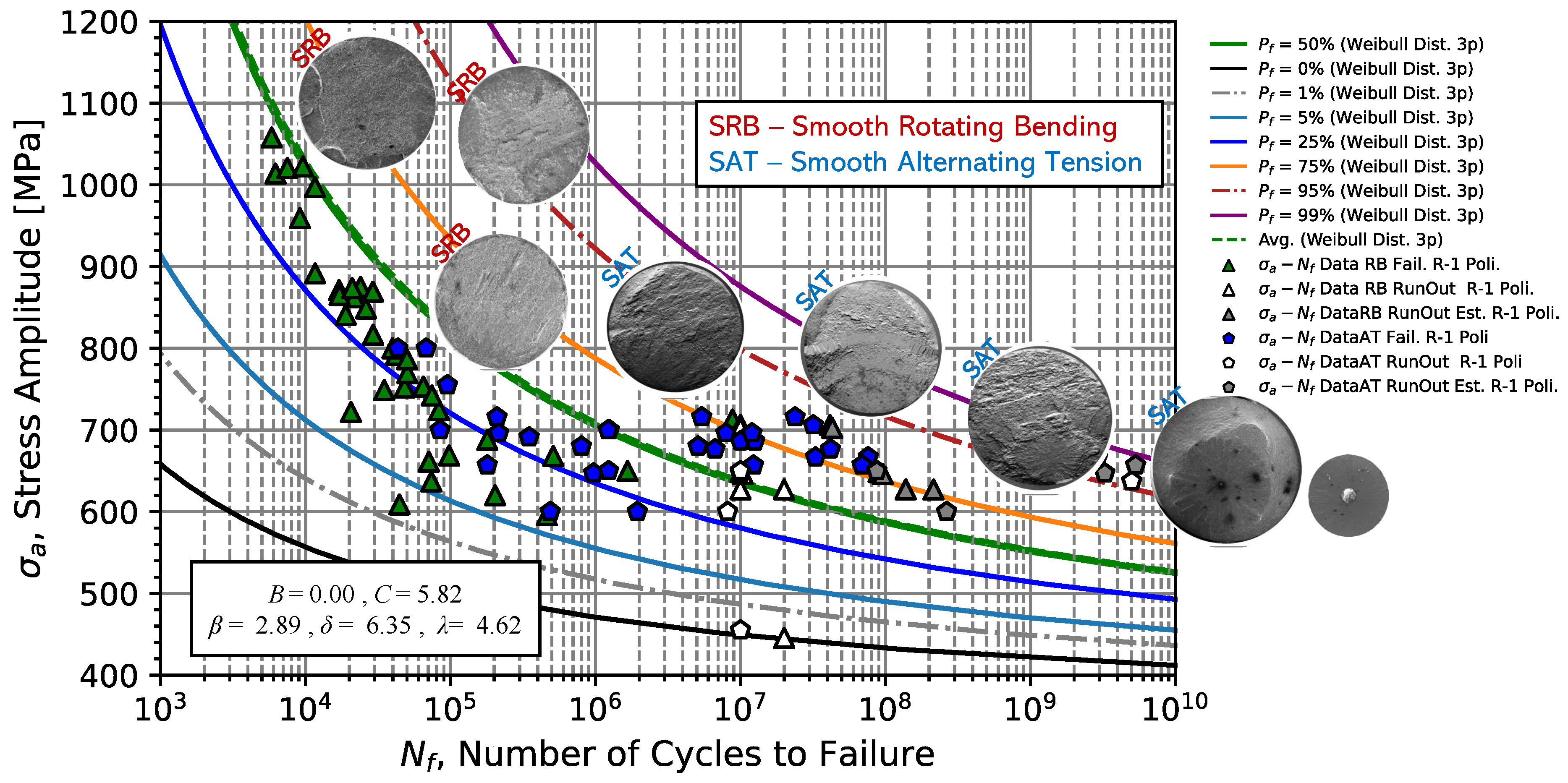
Figure 23 succinctly illustrates the fatigue fracture surfaces observed for different stress amplitude levels from high-cycle to giga-cycle fatigue regime considering the loading type, rotating bending (SRB) and uniaxial tensile/compressive (SAT).
4.5. Non-metallic Inclusions Analysis
To obtain a better characterization of the fracture surfaces of specimens with cracks initiated by inclusions, an EDS analysis was performed on the zones where non-metallic inclusions are visible.
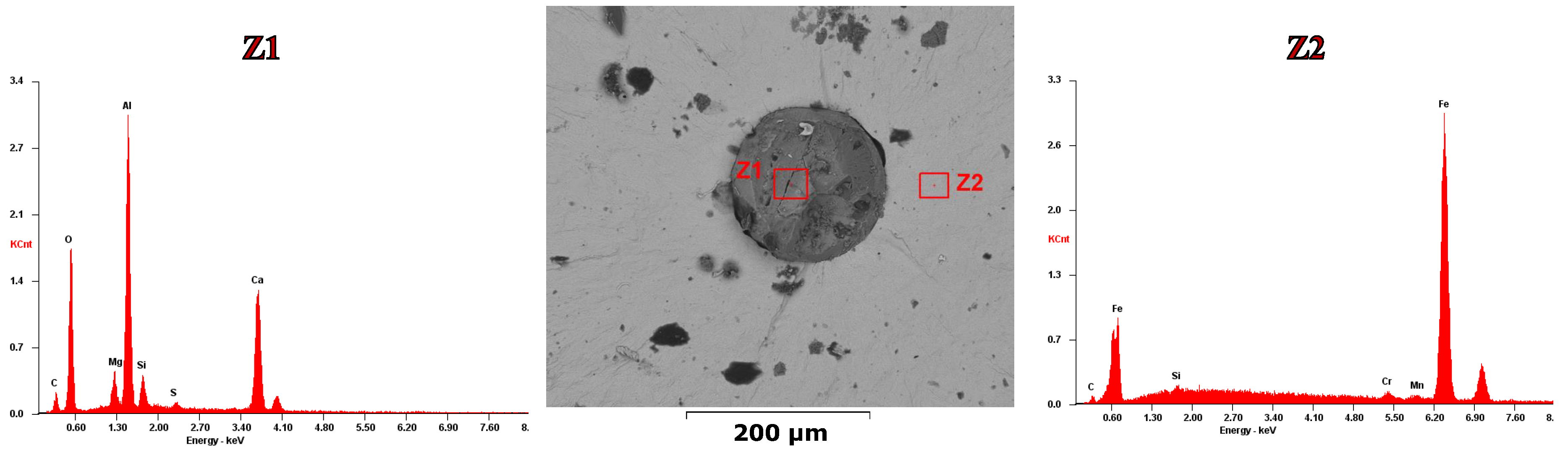
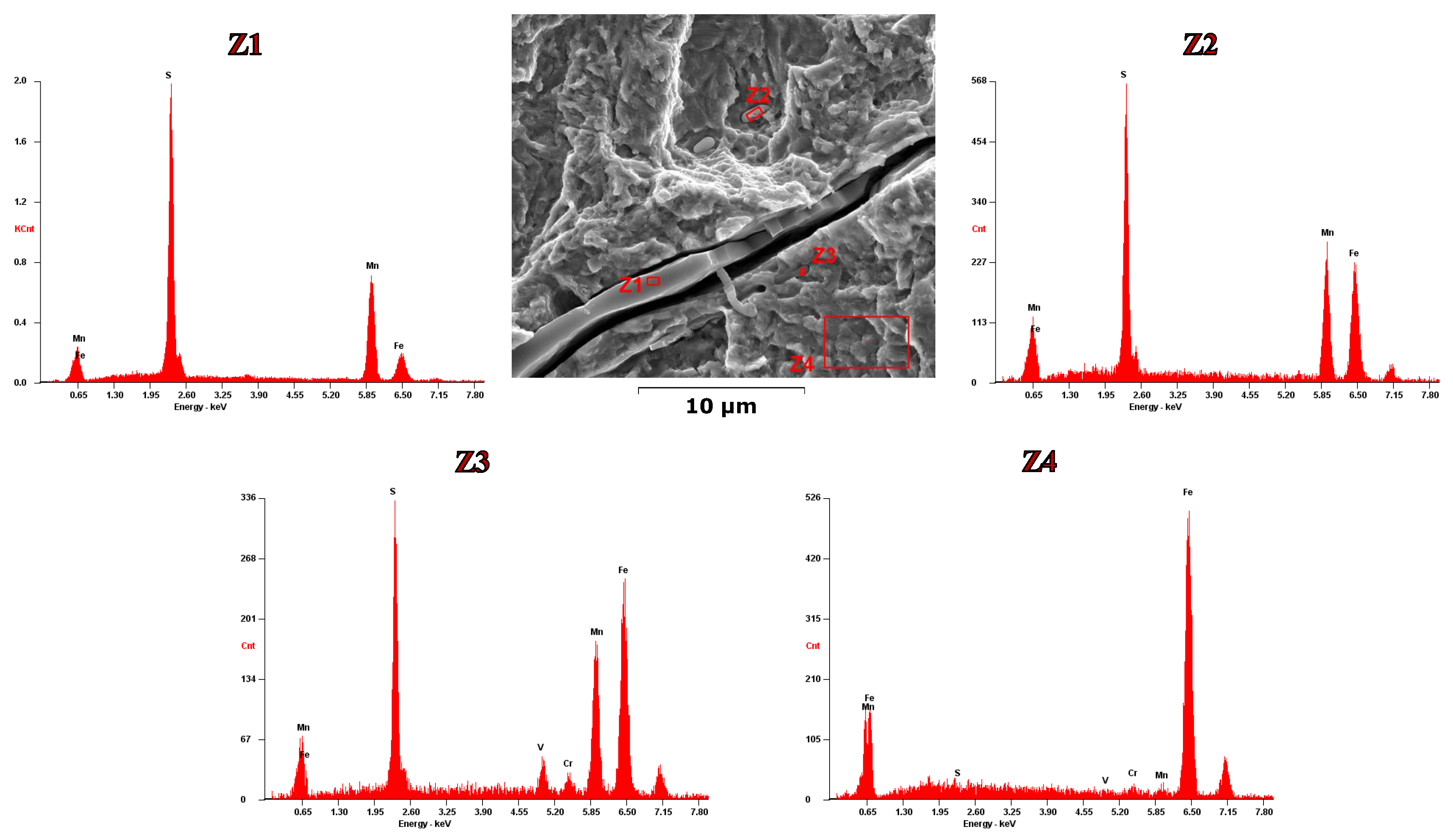
Figure 24 and
Figure 25 present two types of common non-metallic inclusion geometries. In the first case (
Figure 24), the fracture surface exhibits a spherical inclusion of approximately 170
m in diameter. This inclusion shape is usually found by the compound Al
3O
2 [
6]. According to the EDS analysis, the presence of a cluster Al
3O
2 and CaO is verified. Furthermore, amounts of Mn and Si indicate the presence of manganese sulfides. In contrast to the constituents present in zone Z1, zone Z2 presents the constituents of the metal matrix of 51CrV4 steel.
About the non-metallic inclusions with elongated geometry such as the one shown in the fracture surface of
Figure 21D, the EDS analysis was performed in an area far from the initiation zone where the inclusion was found. The EDS analysis revealed that this inclusion is a manganese silicate (see in
Figure 25 the chemical composition analysis for zone Z1). From the micrograph, it is visible a de-cohesion at the metallic matrix-inclusion interface and the fracture of the non-metallic inclusion. This type of geometry of non-metallic inclusions is elongated according to the lamination rolling direction and therefore is easily found when the tested specimens are obtained perpendicular to the rolling direction. Inspecting the zones around this inclusion, other MnS inclusions are found, but with smaller dimensions in the order of 4
m (see in
Figure 25 the chemical composition analysis for zones Z2 and Z3).
5. Conclusions
In this paper, probabilistic fatigue prediction curves based on SN and CFC models are suggested for the fatigue strength of spring steel, 51CrV4 under reversible cycling loading (R = - 1). This steel grade is applied to a wide range of components, which in the case of railway rolling stock components is often used in the production of leaf springs.
Since leaf springs operated under bending conditions, rotating bending fatigue tests were initially performed at low frequency (25 Hz) up to the infinite life of 107 cycles. The initial fatigue resistance analysis was carried out using SN curves, which resulted in a coefficient = 3433.34 MPa and an exponent = - 0.1369 and a determination coefficient of 0.5662, for rotating bending fatigue tests. In order to extend the strength curve to lives greater than 107 cycles, 51CrV4 steel was tested to 109 cycles using high-frequency fatigue machines operating at 20 kHz with tensile loads/ uniaxial compression in the fatigue limit region. The batch of data obtained resulted in an SN curve with the coefficient of 1149.03 MPa and exponent of -0.0314 with a very low value of (0.2305), characteristic of the fatigue life scatter in the region of the test. Since material testing at high-frequency tends to increase the material’s mechanical and fatigue resistance, uniaxial tension/compression load tests at lower frequency (150 Hz) were also carried out, with curves with a coefficient = 2355.20 MPa, an exponent = - 0.0934, slightly larger, and also larger (0.4361), also largely due to the range of stress amplitude and fatigue life tested. From the frequency effect analysis with a combination of 20 kHz failure data (corrected) with the data tested at 150 Hz, it was verified that the material did not present a significant frequency effect, with an adjusted SN curve of = 1572 .0 MPa is an exponent = - 0.0551, with = 0.1738.
Since the applied stress amplitude approaches the fatigue limit region, the value of suggests the use of other prediction models is low. In this paper, the CFC (3-parameter Weibul) model was considered in the analysis of rotating bending and uniaxial tension/compression conditions with combined data. According to the analyses carried out, under rotating bending conditions, the Weibul parameters are = 1.88, = 3.90, and = 8.86, with B = 0.0 and C = 5.57, while under uniaxial tension/compression fatigue loads, the failure data is fitted by = 2.89, = 7.21, and = 5.70, with B = 0.0 and C = 5.57.
From the analysis of the combined fatigue model, it was found that the SN model (with = 1904.76 MPa, an exponent = - 0.0703, and = 0.43) is more conservative, not suitable for prediction of fatigue life in the fatigue limit region (stress amplitudes close to = 655.16 MPa), and with the average curve not correctly fitting the failure data. Contrary to the SN model, the CFC model combined with the Weibull parameters ( = 2.89, = 6.35, and = 4.62, B = 0.0, and C = 5.82) results in a more representative model of the material failure probability curve with an estimate for the fatigue limit given by the hyperbolic curve of 338 MPa (1/2 of of the SN model).
Lastly, the fracture surfaces analysed in the experimental campaign of all fatigue tests using SEM and EDS, for different stress amplitude levels in the HFC and VHCF zone revealed that under conditions of rotating bending, multiple crack initiation occurs for stress amplitudes greater than 800 MPa, and for stresses lower than about 600 MPa, only a single crack is found. For stress amplitudes greater than 670 MPa, under axial uniform stress loading, single crack initiation occurs preferentially from the surface, however, if the stress amplitudes are low enough, a mixed failure zone with crack initiation from non-metallic inclusions starts appearing. Regarding the type of non-metallic inclusions found on the fracture surfaces, the EDS analysis revealed the appearance of Al3O4, CaO, and MnS with and without the formation of the FGA zone. Analysis of different samples of fracture surfaces for different levels of stress amplitude revealed the trend in crack initiation modes expected, which means that very high loads result in multiple crack initiation, medium loads result in single cracks, and very low loads occur surface single cracks or internal cracks.
In summary, the research carried out and presented in this article suggests the use of the combined CFC model to predict the fatigue life of components made with 51CrV4 steel (in quenched and tempered conditions) when the stress amplitudes are uniaxial tension/compression or bending.
Author Contributions
Conceptualization, Gomes V.M.G. and Fiorentin, F.K.; methodology, Gomes V.M.G., Fiorentin, F.K., Dantas, R., and Silva, F.G.A.; software, Gomes V.M.G., Fiorentin, F.K., Dantas, R. and Silva, F.G.A.; validation, Gomes V.M.G., Fiorentin, F.K., Dantas, R., Correia J.A.F.O. and de Jesus A.M.P.; formal analysis, Gomes V.M.G., Fiorentin, F.K., Dantas, R. and ; investigation, Gomes V.M.G., Fiorentin, F.K., Dantas, R. and Silva, F.G.A.; resources, Correia J.A.F.O. and de Jesus A.M.P.; data curation, Gomes V.M.G., Fiorentin, F.K., and Dantas, R.; writing—original draft preparation, Gomes V.M.G.; writing—review and editing, Gomes V.M.G., Fiorentin, F.K., Dantas, R., Silva, F.G.A., Correia J.A.F.O. and de Jesus A.M.P.; visualization, Gomes V.M.G.; supervision, Silva, F.G.A., Correia J.A.F.O. and de Jesus A.M.P.; project administration, de Jesus A.M.P.; funding acquisition, de Jesus A.M.P.
Institutional Review Board Statement
Not applicable
Informed Consent Statement
Not applicable
Data Availability Statement
The data presented in this study are available on request from the corresponding author. The data are not publicly available due to privacy restrictions.
Acknowledgments
The authors also want to express a special thanks to the Doctoral Programme iRail - Innovation in Railway Systems and Technologies funded by the Portuguese Foundation for Science and Technology, IP (FCT) through the PhD grant (PD/BD/143141/2019); and the following Research Projects: GCYCLEFAT - Giga-cycle fatigue behaviour of engineering metallic alloys, with reference PTDC/EME-EME/7678/2020; FERROVIA 4.0, with reference POCI-01-0247-FEDER-046111, co-financed by the European Regional Development Fund (ERDF), through the Operational Programme for Competitiveness and Internationalization (COMPETE 2020), under the PORTUGAL 2020 Partnership Agreement; SMARTWAGONS - DEVELOPMENT OF PRODUCTION CAPACITY IN PORTUGAL OF SMART WAGONS FOR FREIGHT with reference nr. C644940527-00000048, investment project nr.27 from the Incentive System to Mobilising Agendas for Business Innovation, funded by the Recovery and Resilience Plan and by European Funds NextGeneration EU; and PRODUCING RAILWAY ROLLING STOCK IN PORTUGAL, with reference nr. C645644454-00000065, investment project nr. 55 from the Incentive System to Mobilising Agendas for Business Innovation, funded by the Recovery and Resilience Plan and by European Funds NextGeneration EU. And a final thank you to CEMUP, "Centro de Materiais da Universidade do Porto", and respective technical staff for carrying out the scanning electron microscopy tests.
Conflicts of Interest
The authors declare no conflict of interest.
References
- Zerbst, U.; Beretta, S.; Köhler, G.; Lawton, A.; Vormwald, M.; Beier, H.; Klinger, C.; Černý, I.; Rudlin, J.; Heckel, T.; et al. Safe life and damage tolerance aspects of railway axles – A review. Engineering Fracture Mechanics 2013, 98, 214–271. [Google Scholar] [CrossRef]
- Zhao, Y.; Yang, B.; Feng, M.; Wang, H. Probabilistic fatigue S–N curves including the super-long life regime of a railway axle steel. International Journal of Fatigue 2009, 31, 1550–1558. [Google Scholar] [CrossRef]
- Xiu, R.; Spiryagin, M.; Wu, Q.; Yang, S.; Liu, Y. Fatigue life assessment methods for railway vehicle bogie frames. Engineering Failure Analysis 2020, 116, 104725. [Google Scholar] [CrossRef]
- Kassner, M. Fatigue strength analysis of a welded railway vehicle structure by different methods. International journal of fatigue 2012, 34, 103–111. [Google Scholar] [CrossRef]
- Bathias, C.; Paris, P.C. Gigacycle Fatigue in Mechanical Practice, 1ª ed.; 2005. [Google Scholar]
- Murakami, Y. Metal Fatigue: Effects of Small Defects and Nonmetallic Inclusions.; Elsevier Science: Kyushu University, Japan, 2002. [Google Scholar]
- Furuya, Y.; Matsuoka, S.; Abe, T.; Yamaguchi, K. Gigacycle fatigue properties for high-strength low-alloy steel at 100 Hz, 600 Hz, and 20 kHz. Scripta Materialia 2002, 46, 157–162. [Google Scholar] [CrossRef]
- Takeuchi, E.; Furuya, Y.; Nagashima, N.; Matsuoka, S. The effect of frequency on the giga-cycle fatigue properties of a Ti–6Al–4V alloy. Fatigue & Fracture of Engineering Materials & Structures 2008, 31, 599–605. [Google Scholar] [CrossRef]
- Newman, J. Fatigue and Crack-growth Analyses under Giga-cycle Loading on Aluminum Alloys. Procedia Engineering 2015, 101, 339–346, 3rd International Conference on Material and Component Performance under Variable Amplitude Loading, VAL 2015. [Google Scholar] [CrossRef]
- Nonaka, I.; Setowaki, S.; Ichikawa, Y. Effect of load frequency on high cycle fatigue strength of bullet train axle steel. International journal of fatigue 2014, 60, 43–47. [Google Scholar] [CrossRef]
- Saucedo, L.; Yu, R.C.; Medeiros, A.; Zhang, X.; Ruiz, G. A probabilistic fatigue model based on the initial distribution to consider frequency effect in plain and fiber reinforced concrete. International Journal of Fatigue 2013, 48, 308–318. [Google Scholar] [CrossRef]
- Castillo, E.; Fernández-Canteli, A.; Blasón, S.; Khatibi, G.; Czerny, B.; Zareghomsheh, M. Step-by-Step Building of a Four Dimensional Fatigue Compatible Regression Model including Frequencies. Open Journal of Statistics 2021, 11, 1072–1096. [Google Scholar] [CrossRef]
- Schneider, N.; Bödecker, J.; Berger, C.; Oechsner, M. Frequency effect and influence of testing technique on the fatigue behaviour of quenched and tempered steel and aluminium alloy. International Journal of Fatigue 2016, 93, 224–231. [Google Scholar] [CrossRef]
- Guennec, B.; Ueno, A.; Sakai, T.; Takanashi, M.; Itabashi, Y. Effect of the loading frequency on fatigue properties of JIS S15C low carbon steel and some discussions based on micro-plasticity behavior. International journal of fatigue 2014, 66, 29–38. [Google Scholar] [CrossRef]
- Palin-Luc, T.; Jeddi, D. The gigacycle fatigue strength of steels: a review of structural and operating factors. Procedia Structural Integrity 2018, 13, 1545–1553. [Google Scholar] [CrossRef]
- Kovacs, S.; Beck, T.; Singheiser, L. Influence of mean stresses on fatigue life and damage of a turbine blade steel in the VHCF-regime. International Journal of Fatigue 2013, 49, 90–99. [Google Scholar] [CrossRef]
- Furuya, Y. Size effects in gigacycle fatigue of high-strength steel under ultrasonic fatigue testing. Procedia Engineering 2010, 2, 485–490. [Google Scholar] [CrossRef]
- Furuya, Y. Specimen size effects on gigacycle fatigue properties of high-strength steel under ultrasonic fatigue testing. Scripta Materialia 2008, 58, 1014–1017. [Google Scholar] [CrossRef]
- Hilgendorff, P.M.; Grigorescu, A.; Zimmermann, M.; Fritzen, C.P.; Christ, H.J. Simulation of deformation-induced martensite formation and its influence on the resonant behavior in the very high cycle fatigue (VHCF) regime. Procedia materials science 2014, 3, 1135–1142. [Google Scholar] [CrossRef]
- Klein Fiorentin, F.; Reis, L.; Lesiuk, G.; Reis, A.; de Jesus, A. A Predictive Methodology for Temperature, Heat Generation and Transfer in Gigacycle Fatigue Testing. Metals 2023, 13, 492. [Google Scholar] [CrossRef]
- Papadopoulos, I.V.; Panoskaltsis, V.P. Invariant formulation of a gradient dependent multiaxial high-cycle fatigue criterion. Engineering Fracture Mechanics 1996, 55, 513–528. [Google Scholar] [CrossRef]
- Tomaszewski, T.; Strzelecki, P.; Mazurkiewicz, A.; Musiał, J. Probabilistic estimation of fatigue strength for axial and bending loading in high-cycle fatigue. Materials 2020, 13, 1148. [Google Scholar] [CrossRef]
- Pascual, F.G.; Meeker, W.Q. Estimating Fatigue Curves With the Random Fatigue-Limit Model. Technometrics 1999, 277–289. [Google Scholar] [CrossRef]
- Gomes, V.M.; Lesiuk, G.; Correia, J.A.; De Jesus, A.M. Fatigue Crack Propagation of 51CrV4 Steels for Leaf Spring Suspensions of Railway Freight Wagons. Materials 2024, 17, 1831. [Google Scholar] [CrossRef] [PubMed]
- Gomes, V.M.; Souto, C.D.; Correia, J.A.; de Jesus, A.M. Monotonic and Fatigue Behaviour of the 51CrV4 Steel with Application in Leaf Springs of Railway Rolling Stock. Metals 2024, 14, 266. [Google Scholar] [CrossRef]
- EN1993-1-9. Eurocode 3: Design of Steel Structures - Part 1-9: Fatigue. European Committee for Standardization 2005.
- Basquin, O.H. The exponential law of endurance tests. Proceedings of the American Society for Testing and Materials 1910, 10, 625–630. [Google Scholar]
- Castillo, E.; Fernández-Canteli, A. A Unified Statistical Methodology for Modeling Fatigue Damage; Springer: Netherlands, 2009. [Google Scholar] [CrossRef]
- ASTME732. Standard Practice for Statistical Analysis of Linear or Linearized Stress-Life (S-N) and Strain-Life (ε-N) Fatigue Data. Annual Book of ASTM Standards 3 2004, 1, 1–7. [Google Scholar]
- Strzelecki, P. Determination of fatigue life for low probability of failure for different stress levels using 3-parameter Weibull distribution. International Journal of Fatigue 2021, 145, 106080. [Google Scholar] [CrossRef]
- Ai, Y.; Zhu, S.; Liao, D.; Correia, J.; Souto, C.; De Jesus, A.; Keshtegar, B. Probabilistic modeling of fatigue life distribution and size effect of components with random defects. International Journal of Fatigue 2019, 126, 165–173. [Google Scholar] [CrossRef]
- Li, H.; Wen, D.; Lu, Z.; Wang, Y.; Deng, F. Identifying the probability distribution of fatigue life using the maximum entropy principle. Entropy 2016, 18, 111. [Google Scholar] [CrossRef]
- Rathod, V.; Yadav, O.P.; Rathore, A.; Jain, R. Probabilistic modeling of fatigue damage accumulation for reliability prediction. Journal of Quality and Reliability Engineering 2011, 2011. [Google Scholar] [CrossRef]
- Doh, J.; Lee, J. Bayesian estimation of the lethargy coefficient for probabilistic fatigue life model. Journal of Computational Design and Engineering 2018, 5, 191–197. [Google Scholar] [CrossRef]
- Chabod, A.; Czapski, P.; Aldred, J.; Munson, K. Probabilistic fatigue and reliability simulation. Procedia Structural Integrity 2019, 19, 150–167. [Google Scholar] [CrossRef]
- Wu, Y.L.; Zhu, S.P.; Liao, D.; Correia, J.A.; Wang, Q. Probabilistic fatigue modeling of notched components under size effect using modified energy field intensity approach. Mechanics of Advanced Materials and Structures 2022, 29, 6379–6389. [Google Scholar] [CrossRef]
- Correia, J. An Integral Probabilistic Approach for Fatigue Lifetime Prediction of Mechanical And Structural Components. PhD thesis, Faculty of Engineering of the University of Porto, 2014. [Google Scholar]
- Castillo, E.; Galambos, J. Lifetime regression models based on a functional equation of physical nature. Journal of Applied Probability 1987, 24, 160–169. [Google Scholar] [CrossRef]
- Castillo, E.; Fernández-Canteli, A.; Ruiz-Tolosa, J.; Sarabia, J. Statistical models for analysis of fatigue life of long elements. Journal of engineering mechanics 1990, 116, 1036–1049. [Google Scholar] [CrossRef]
- Castillo, E.; Fernández-Canteli, A. A General Regression Model for Lifetime Evaluation and Prediction. International Journal of Fracture 2001, 107, 117–137. [Google Scholar] [CrossRef]
- Castillo, E.; López-Aenlle, M.; Ramos, A.; Fernández-Canteli, A.; Kieselbach, R.; Esslinger, V. Specimen Length Effect on Parameter Estimation in Modelling Fatigue Strength by Weibull Distribution. International Journal of Fatigue 2006, 28, 1047–1058. [Google Scholar] [CrossRef]
- Castillo, E.; Fernández-Canteli, A.; Ruiz-Ripoll, M.L. A General Model for Fatigue Damage Due to Any Stress History. International Journal of Fatigue 2008, 30, 150–164. [Google Scholar] [CrossRef]
- Fernández-Canteli, A.; Przybilla, C.; Nogal, M.; Aenlle, M.L.; Castillo, E. ProFatigue: A software program for probabilistic assessment of experimental fatigue data sets. Procedia Engineering 2014, 74, 236–241. [Google Scholar] [CrossRef]
- Lee, C.; Lee, K.; Li, D.; Yoo, S.; Nam, W. Microstructural influence on fatigue properties of a high-strength spring steel. Materials Science and Engineering: A 1998, 241, 30–37. [Google Scholar] [CrossRef]
- Metallic materials-tensile testing-Part 1: Method of test at ambient temperature. ISO6892-1; 2009.
- Metallic materials - Rotating bar bending fatigue testing. ISO1143; International Standard Organization, 2010.
- Qualitest. Resonant fatigue testing machines. Available online: https://www.worldoftest.com/resonant-fatigue-testing-machines (accessed on 8 June 2022).
- RUMUL. Rumul Equipment. Available online: https://www.rumul.ch/index.php?lang_choose=1 (accessed on 7 June 2022).
- ASTME466. Standard Practice For Conducting Force Controlled Constant Amplitude Axial Fatigue Tests Of Metallic Materials. Book of Standards Vol. 03.01 2021, 7. [CrossRef]
- Li, W.; Sakai, T.; Li, Q.; Lu, L.; Wang, P. Effect of loading type on fatigue properties of high strength bearing steel in very high cycle regime. Materials Science and Engineering: A 2011, 528, 5044–5052. [Google Scholar] [CrossRef]
- Malikoutsakis, M.; Makris, I.; Pagonas, A.; Savaidis, G. Characterization and performance of high strength steel 51CrV4 under cyclic loading. In Proceedings of the MATEC Web of Conferences. EDP Sciences, Vol. 349; 2021; p. 02008. [Google Scholar] [CrossRef]
- Shigley, J.E.; Mischke, C.R.; Brown Jr, T.H. Standard handbook of machine design; McGraw-Hill Education, 2004. [Google Scholar]
Figure 1.
Two-axle wagon suspension with a parabolic leaf spring.
Figure 1.
Two-axle wagon suspension with a parabolic leaf spring.
Figure 2.
Typical microstructure of the chromium-vanadium alloyed steel for all tested specimens [
25].
Figure 2.
Typical microstructure of the chromium-vanadium alloyed steel for all tested specimens [
25].
Figure 3.
Rotating bending fatigue testing machine (simple bending).
Figure 3.
Rotating bending fatigue testing machine (simple bending).
Figure 4.
Geometry of the smooth fatigue specimen for rotating bending loading. Left: Sample of the actual specimen showing the detail (Dt.A) of the finishing in the analysis zone: Dt. A1 - polished, Dt. A2 - unpolished. Right: Rendered image of the CAD model showing the dimensions for the definition of the specimen geometry.
Figure 5.
Representation of Shimadzu’s machine, its structure and testing specimen with the cooling system.
Figure 5.
Representation of Shimadzu’s machine, its structure and testing specimen with the cooling system.
Figure 6.
Geometry of the fatigue specimen for ultrasonic uniaxial tension/compression testing in the Shimadzu’s machine. Left: Sample of the actual specimen showing the detail (Dt. A) of the finishing in the analysis zone: Dt. A - polished. Right: Rendered image of the CAD model showing the dimensions for the definition of the specimen geometry.
Figure 7.
Rumul’s machine and the testing specimen installed.
Figure 7.
Rumul’s machine and the testing specimen installed.
Figure 8.
Geometry of the smooth fatigue specimen for uniaxial tension/compression testing in the Rumul machine: Left: Rendered image of the CAD model showing the dimensions for definition of the specimen geometry, and Right: Sample of the actual specimen.
Figure 8.
Geometry of the smooth fatigue specimen for uniaxial tension/compression testing in the Rumul machine: Left: Rendered image of the CAD model showing the dimensions for definition of the specimen geometry, and Right: Sample of the actual specimen.
Figure 9.
SN curve for smooth fatigue specimens under rotating bending loading conditions with turned surface finishing. (R - stress ratio; - Probability of failure; RB - Rotating Bending)
Figure 9.
SN curve for smooth fatigue specimens under rotating bending loading conditions with turned surface finishing. (R - stress ratio; - Probability of failure; RB - Rotating Bending)
Figure 10.
SN curve for smooth fatigue specimens under rotating bending loading conditions with polished plus turned surface finishing. (R - stress ratio; - Probability of failure; RB - Rotating Bending; Poli. - Polished specimen; Turn -Turned specimens)
Figure 10.
SN curve for smooth fatigue specimens under rotating bending loading conditions with polished plus turned surface finishing. (R - stress ratio; - Probability of failure; RB - Rotating Bending; Poli. - Polished specimen; Turn -Turned specimens)
Figure 11.
SN curve for smooth fatigue specimens with polished surface finishing under subsonic tension/compression fatigue loading conditions. (R - stress ratio; - Probability of failure; AT(150Hz) - specimen under axial tension at 150 Hz)
Figure 11.
SN curve for smooth fatigue specimens with polished surface finishing under subsonic tension/compression fatigue loading conditions. (R - stress ratio; - Probability of failure; AT(150Hz) - specimen under axial tension at 150 Hz)
Figure 12.
SN curve for smooth fatigue specimens with polished surface finishing under ultrasonic tension/compression fatigue loading conditions. (R - stress ratio; - Probability of failure; AT(20kHz) - specimen under axial tension at 20 kHz)
Figure 12.
SN curve for smooth fatigue specimens with polished surface finishing under ultrasonic tension/compression fatigue loading conditions. (R - stress ratio; - Probability of failure; AT(20kHz) - specimen under axial tension at 20 kHz)
Figure 13.
Comparison of fatigue data obtained for the fatigue life of spring steel under uniaxial tension/compression tests. (R - stress ratio; - Probability of failure; AT(150Hz) - specimen under axial tension at 150 Hz; AT(20kHz) - specimen under axial tension at 20 kHz)
Figure 13.
Comparison of fatigue data obtained for the fatigue life of spring steel under uniaxial tension/compression tests. (R - stress ratio; - Probability of failure; AT(150Hz) - specimen under axial tension at 150 Hz; AT(20kHz) - specimen under axial tension at 20 kHz)
Figure 14.
Comparison of fatigue data obtained from fatigue tests of spring steel in uniaxial tensile tests at 150 Hz and 20 kHz considering corrected nominal stresses for frequency effect. (R - stress ratio; - Probability of failure; AT(150Hz) - specimen under axial tension at 150 Hz; AT(20kHz) - specimen under axial tension at 20 kHz)
Figure 15.
PSN field for smooth specimens under fatigue rotating bending loadings. (R - stress ratio; - Probability of failure; Est- estimation for run-out data; RB(25Hz) - smooth specimens under rotating bending at 25 Hz)
Figure 15.
PSN field for smooth specimens under fatigue rotating bending loadings. (R - stress ratio; - Probability of failure; Est- estimation for run-out data; RB(25Hz) - smooth specimens under rotating bending at 25 Hz)
Figure 16.
PSN field curve for smooth specimens under subsonic and ultrasonic fatigue tensile loadings. (R - stress ratio; - Probability of failure; Est- estimation for run-out data; AT(150Hz) - smooth specimens under axial tension at 150 Hz; AT(20kHz) - smooth specimens under axial at 20 kHz)
Figure 16.
PSN field curve for smooth specimens under subsonic and ultrasonic fatigue tensile loadings. (R - stress ratio; - Probability of failure; Est- estimation for run-out data; AT(150Hz) - smooth specimens under axial tension at 150 Hz; AT(20kHz) - smooth specimens under axial at 20 kHz)
Figure 17.
Regression model considering the dataset of rotating bending and axial tensile fatigue loading. (R - stress ratio; - Probability of failure; RB(25Hz) - specimen under rotating bending at 25Hz; AT(150Hz) - specimen under axial tension at 150 Hz; AT(20kHz) - specimen under axial tension at 20 kHz)
Figure 18.
PSN hyperbolic field considering only the rotating bending and tensile loadings. (R - stress ratio; - Probability of failure; Est- estimation for run-out data; RB - smooth specimens under rotating bending; AT - smooth specimens under axial tension)
Figure 18.
PSN hyperbolic field considering only the rotating bending and tensile loadings. (R - stress ratio; - Probability of failure; Est- estimation for run-out data; RB - smooth specimens under rotating bending; AT - smooth specimens under axial tension)
Figure 19.
Comparison between the PSN power and hyperbolic fields from rotating bending and tensile fatigue data. (R - stress ratio; - Probability of failure; Est- estimation for run-out data; RB - smooth specimens under rotating bending; AT - smooth specimens under axial tension)
Figure 19.
Comparison between the PSN power and hyperbolic fields from rotating bending and tensile fatigue data. (R - stress ratio; - Probability of failure; Est- estimation for run-out data; RB - smooth specimens under rotating bending; AT - smooth specimens under axial tension)
Figure 20.
Fracture surfaces for the three stress amplitude regions of the rotating bending specimens: A) = 1057.96 MPa, B) = 1020.62 MPa, C) = 816.56 MPa, D) = 595.67 MPa.
Figure 20.
Fracture surfaces for the three stress amplitude regions of the rotating bending specimens: A) = 1057.96 MPa, B) = 1020.62 MPa, C) = 816.56 MPa, D) = 595.67 MPa.
Figure 21.
Fracture surfaces obtained for different stress amplitude and testing frequencies of specimens under uniaxial test conditions (R = -1.0): A) = 770 MPa (20 kHz), B) = 705 MPa (20 kHz), C) = 670 MPa (20 kHz), D) = 680 MPa (20 kHz), E) = 650 MPa (150 Hz).
Figure 21.
Fracture surfaces obtained for different stress amplitude and testing frequencies of specimens under uniaxial test conditions (R = -1.0): A) = 770 MPa (20 kHz), B) = 705 MPa (20 kHz), C) = 670 MPa (20 kHz), D) = 680 MPa (20 kHz), E) = 650 MPa (150 Hz).
Figure 22.
Comparison of different crack propagation zones of a fish-eye fracture surface. A and B - Close to the non-metallic inclusion, C - Away from the initiation zone.
Figure 22.
Comparison of different crack propagation zones of a fish-eye fracture surface. A and B - Close to the non-metallic inclusion, C - Away from the initiation zone.
Figure 23.
Fatigue fracture surfaces depending on the amplitude stress level from high-cycle up to giga-cycle and for rotating bending (SRB) and uniaxial tension/compression (SAT) loads
Figure 23.
Fatigue fracture surfaces depending on the amplitude stress level from high-cycle up to giga-cycle and for rotating bending (SRB) and uniaxial tension/compression (SAT) loads
Figure 24.
Analysis of the chemical composition of the non-metallic inclusion and the metallic matrix through EDS: Z1 Zone 1, Z2 - Zone 2.
Figure 24.
Analysis of the chemical composition of the non-metallic inclusion and the metallic matrix through EDS: Z1 Zone 1, Z2 - Zone 2.
Figure 25.
Chemical composition analysis of the non-metallic slender inclusions and the matrix through EDS.
Figure 25.
Chemical composition analysis of the non-metallic slender inclusions and the matrix through EDS.
Table 1.
Standard chemical composition of 51CrV4 steel grade in % wt.
Table 1.
Standard chemical composition of 51CrV4 steel grade in % wt.
| Material |
C |
Si |
Mn |
Cr |
V |
S |
Pb |
Fe |
| 51CrV4 EN 1.815 |
0.47-0.55 |
≤0.40 |
0.70-1.10 |
0.90-1.20 |
≤0.10-0.25 |
≤0.025 |
≤0.025 |
96.45-97.38 |
Table 2.
Monotonic mechanical properties obtained of the chromium-vanadium alloyed steel, 51CrV4 [
25].
Table 2.
Monotonic mechanical properties obtained of the chromium-vanadium alloyed steel, 51CrV4 [
25].
|
E |
|
|
|
|
|
[GPa] |
[MPa] |
[MPa] |
[%] |
[%] |
| Average |
|
|
|
7.53 |
34.69 |
| Std. Dev. [] |
|
|
|
|
|
| DIN 51CrV4 (1.8159) |
200 |
1200 |
1350-1650 |
6 |
30 |
Table 3.
Average dimensions of machined and polished smooth specimens used in rotating bending fatigue testing according to ISO 1143 standard [
46].
Table 3.
Average dimensions of machined and polished smooth specimens used in rotating bending fatigue testing according to ISO 1143 standard [
46].
| Finishing |
[mm] |
[mm] |
L [mm] |
[mm] |
[mm] |
D [mm] |
|
[mm] |
M [mm] |
| Polishing |
|
|
|
|
|
12 |
10 |
7.67 |
M5 |
| |
|
|
|
|
|
- |
- |
|
- |
| Turning |
|
|
|
|
|
12 |
10 |
7.62 |
M5 |
| |
|
|
|
|
|
- |
- |
|
- |
| Average |
|
|
|
|
|
12 |
10 |
7.63 |
M5 |
| |
|
|
|
|
|
- |
- |
|
- |
Table 4.
Average dimensions of specimens used in uniaxial fatigue tests in the ultrasonic testing machine.
Table 4.
Average dimensions of specimens used in uniaxial fatigue tests in the ultrasonic testing machine.
|
[mm] |
R
|
[mm] |
L [mm] |
[mm] |
M [mm] |
D [mm] |
| 4.00
|
|
73.02 |
|
13.51 |
|
10.00 |
Table 5.
Average dimensions of specimens used in fatigue uniaxial tension/compression tests in accordance with the manufacturer and standard ASTM E4-621 [
49] for fatigue axial-force testing.
Table 5.
Average dimensions of specimens used in fatigue uniaxial tension/compression tests in accordance with the manufacturer and standard ASTM E4-621 [
49] for fatigue axial-force testing.
|
[mm] |
|
D [mm] |
[mm] |
L [mm] |
M [mm] |
R [mm] |
| 7.05
|
|
9 |
|
110 |
|
36.6 |
Table 6.
Summary of Basquin SN model, based on nominal amplitude stress for rotating bending conditions.
Table 6.
Summary of Basquin SN model, based on nominal amplitude stress for rotating bending conditions.
| Surface Finishing |
Turned |
Polished |
Turned + Polished |
| Fatigue Limit,
|
660.8 |
- |
667.3 |
| Strength Coefficient,
|
|
2005.68 |
3433.347 |
| Strength Exponent,
|
-0.1460 |
-0.082 |
-0.137 |
| Coefficient of Determination,
|
|
0.5500 |
0.5662 |
| Mean Square Error,
|
0.115 |
0.370 |
0.201 |
| Coefficient of Interception,
|
24.39 |
25.832 |
25.83 |
| Coefficient of Slope,
|
-6.831 |
-7.306 |
-7.306 |
| Average Ind. Var, , |
2.890 |
2.898 |
2.898 |
| Average Dep. Var, , |
4.647 |
4.662 |
4.662 |
| Std. Dep. Var, , |
0.6061 |
0.6714 |
0.6714 |
Table 7.
Summary of Basquin SN model, based on stress amplitude for rotating bending and uniaxial tension/compression test conditions ( = - 1.0).
Table 7.
Summary of Basquin SN model, based on stress amplitude for rotating bending and uniaxial tension/compression test conditions ( = - 1.0).
| Testing |
Subsonic |
Subsonic |
Ultrasonic |
| Conditions |
Rotating Bending |
Tensile |
Tensile |
| Frequency, f
|
25 |
150 |
20 000 |
| Strength Coefficient,
|
3433.347 |
2355.20 |
1149.03 |
| Strength Exponent,
|
-0.137 |
-0.0934 |
-0.0314 |
| Coefficient of Determination,
|
0.5662 |
0.4361 |
0.2305 |
| Mean Square Error,
|
0.201 |
0.3057 |
1.149 |
| Coefficient of Interception,
|
25.83 |
36.12 |
97.37 |
| Coefficient of Slope,
|
-7.306 |
-10.71 |
-31.82 |
| Average Ind. Var,
|
2.898 |
2.837 |
2.842 |
| Average Dep. Var,
|
4.662 |
5.725 |
6.936 |
| Std. Dep. Var,
|
0.6714 |
0.6941 |
1.1922 |
Table 8.
Summary of the comparison of the Basquin SN models considering the effect of frequency on rotating bending and tension/compression fatigue testing data.
Table 8.
Summary of the comparison of the Basquin SN models considering the effect of frequency on rotating bending and tension/compression fatigue testing data.
| |
Subsonic (T) |
Subsonic (T) |
Subsonic (RB + T) |
| Testing |
+ Ultrasonic |
+ Ultrasonic |
+ Ultrasonic |
| Conditions |
Effective (T) |
Nominal (T) |
Nominal (T) |
| Fatigue Limit,
|
- |
649.51 |
655.16 |
| Strength Coefficient,
|
1888.0 |
1572.0 |
1904.76 |
| Strength Exponent,
|
-0.0664 |
-0.0551 |
-0.0703 |
| Coefficient of Determination,
|
0.1202 |
0.1738 |
0.4300 |
| Mean Square Error,
|
0.201 |
1.2191 |
1.0441 |
| Coefficient of Interception,
|
25.83 |
36.122 |
88.64 |
| Coefficient of Slope,
|
-7.306 |
-10.71 |
-28.74 |
| Average Ind. Var, , |
2.898 |
2.8350 |
2.8445 |
| Average Dep. Var, , |
6.55764 |
5.725 |
6.882 |
| Std. Dep. Var, , |
1.1949 |
0.6941 |
1.009 |
Table 9.
Summary of the comparison of estimators for the 3-parameters Weibull distribution on smooth specimens under rotating bending and tensile conditions fully-reversed fatigue testing data. (RB - Rotating bending; AT - Axial tension)
Table 9.
Summary of the comparison of estimators for the 3-parameters Weibull distribution on smooth specimens under rotating bending and tensile conditions fully-reversed fatigue testing data. (RB - Rotating bending; AT - Axial tension)
| Testing |
Subsonic (RB) |
Subsonic (AT) |
Subsonic (RB+AT) |
| Conditions |
|
+ Ultrasonic (AT) |
+ Ultrasonic (AT) |
| Vert. Asymptote, B
|
0.00 (1 [cycle]) |
0.00 (1 [cycle]) |
0.00 (1 [cycle]) |
| Hor. Asymptote, C
|
5.57 (261.0 [MPa]) |
5.77 (319.1 [MPa]) |
5.82 (338.4 [MPa]) |
| Shape Par.,
|
1.88 |
2.89 |
2.89 |
| Scale Par.,
|
3.90 |
7.21 |
6.35 |
| Location Par.,
|
8.86 |
5.70 |
4.62 |
| Average Rand. Var. v,
|
12.32 |
12.13 |
10.28 |
| Std. Rand. Var. v,
|
3.661 |
5.836 |
4.527 |
| Quantile Var. v,
|
12.07 |
12.05 |
10.21 |
|
Disclaimer/Publisher’s Note: The statements, opinions and data contained in all publications are solely those of the individual author(s) and contributor(s) and not of MDPI and/or the editor(s). MDPI and/or the editor(s) disclaim responsibility for any injury to people or property resulting from any ideas, methods, instructions or products referred to in the content. |
© 2025 by the authors. Licensee MDPI, Basel, Switzerland. This article is an open access article distributed under the terms and conditions of the Creative Commons Attribution (CC BY) license (http://creativecommons.org/licenses/by/4.0/).