1. Introduction
Recommender systems are of vital importance in addressing the issue of information overload. Traditional models are susceptible to exposure or selection bias, which can result in suboptimal outcomes. This is because users are typically only able to evaluate a limited number of items and lack comprehensive knowledge of their preferences. In the context of recommender systems, selection bias can be defined as the phenomenon in which users select items that do not accurately reflect their true interests or preferences. It is essential to recognize that user recommendations may not always be impartial and may contain subjective evaluations. It is important to note that users may exhibit bias towards certain items for a variety of reasons. Consequently, the recommendations generated by the recommender system may be influenced by selection bias, resulting in recommendations that do not accurately reflect the user’s actual preferences [
1,
2,
3,
4].
The presence of selection bias in recommender systems can give rise to a number of problematic outcomes. The presence of selection bias can have a detrimental impact on the performance of recommender systems. This can result in a reduction in accuracy and an overspecialisation of recommendations [
5] , as they may reflect users’ selection preferences rather than their actual interests. In order to solve the above problems, a reliable method has been used in the past, i.e., conduct of online randomised experiments. However, this may have a detrimental impact on the user experience due to the extended time required to occupy the business traffic. In contrast to online randomised experiments, several offline debiasing methods have been developed in recent years, including the popular inverse propensity scoring (IPS) [
6] strategy. While existing IPS-based debiasing methods improve recommendations over methods that ignore the effects of bias, two significant limitations were identified. The application of IPS-based debiasing to recommendations assumes that (1) the effect of selection bias is static over time and (2) user preferences remain constant as items are used. When selection bias and user preferences are dynamic, that is to say, when they change over time, the current IPS-based approach is unable to remove recommendation bias [
7].
Concurrently, the concepts pertaining to sentiment bias as elucidated by the most recent research can also be employed to offset the consequences of selection bias [
8,
9]. At present, the utilisation of sentiment analysis to remove sentiment bias and alleviate data sparsity represents a promising approach that is unlikely to give rise to modelling difficulties due to differences in data structures. Some researchers argue that affective bias can be removed by representing users’ opinions on different items as ratings [
10,
11]. Others attempt to rate comments as positive or negative through sentiment analysis methods to help recommend [
12,
13]. It is desirable that user ratings and reviews of the goods consumed at the same time be obtained, as this will enable more accurate recommendations to be made based on comprehensive and authentic opinions.
Therefore, to address the issues of selection bias and sentiment bias,we propose to design a debiased recommendation framework (sentiment classification and temporal dynamic debiased recommendation module ,SCTD) based on sentiment analysis and temporal dynamic debiasing. Specifically, SCTD consists of a sentiment classification scoring module (sentiment classification scoring module,SCS) and a temporal dynamic debiased recommendation module (temporal dynamic debiased recommendation module,TDR).
The main contributions of this paper are as follows:
- (1)
We propose a recommendation framework based on affective bias and temporal dynamic debiasing: the SCTD, which exploits the affective scores of reviews and ratings to obtain the user’s true opinion for recommendation.
- (2)
Capturing dynamic user interests and better capturing real-world user behaviours by alleviating data imbalance and sparsity issues through two modules, SCS and TDR.
- (3)
We conducted extensive experiments on two real datasets (yelp and Amazon), and according to the experimental results, our proposed SCTD recommendation model makes good progress and outperforms traditional debiased models.
2. Related Work
Selection debiased recommendation has become a hot research topic. In this section, we review some of the recent literature on selection biased recommendation methods. This includes how dynamic modelling can mitigate the effects of selection bias, and how mitigating data sparsity for studying sentiment bias can in turn help mitigate selection bias.
2.1. Dynamic Debiased Recommender System
To address dynamic scene debiasing, three common methods are typically employed [
1]: Time Window,Time Decay Function,and Integration-Based Learning.The use of time windows and time decay function for the analysis of recent operations may result in the loss of pertinent information and the introduction of noise. Integration-Based Learning employs a multitude of models, each of which considers a mere fraction of the total behavioural spectrum. To address these issues, one paper proposes a definition of dynamic debiasing [
1]. It is essential to recognise that data is subject to change over time and therefore requires constant updating with the latest modelling techniques in order to reflect its current nature. The article above is predicated on the assumption that selection bias is static and that only dynamic user preference scenarios are modelled, which results in the debiasing approach exhibiting suboptimal performance. In response to the aforementioned issue, some researchers have sought to enhance factor-based collaborative filtering algorithms by incorporating temporal features [
14]. They have proposed that the temporal model is more effective than the static model. A challenge persists, as existing collaborative filtering algorithms are static models, wherein relationships are assumed to be fixed at different times. However, it is often the case that relational data evolves over time, exhibiting strong temporal patterns. A paper presented at WSDM ’22 [
7] made the theoretical assumption and proved that existing debiasing methods are no longer unbiased when both selection bias and user preferences are dynamic.
Thus, the current problems that need to be solved in this research direction can be split into: problem of selection bias, and debiased in dynamic scenes. Currently how to solve the problem of selection bias mainstream are data filling (Data imputation) and reverse tendency weighting (Propensity score). The mainstream method of data imputation suffers from empirical errors due to improper designation of the missing data model or inaccurate estimation of the rating value.The performance of IPS-based models depends on the accuracy of propensities.Therefore, previous studies have used heuristic optimisation schemes such as directly populating missing values. Such methods are subject to empirical errors due to improperly specified missing data model or inaccurate score estimation.Currently, the use of propensity scores in training recommendation models is a more common method to mitigate selection bias. The problem faced by propensity scores is that they directly target IPS-based unbiased estimators and optimise specific Iosses, but formulating accurate propensity scores is very rigorous and the performance of IPS-based models depends on the accuracy of the propensity. Propensity score based methods have large variance and can lead to non-optimal results.
2.2. Sentiment Bias
Sentiment bias refers to the bias that exists directly between comments and evaluations [
15]. Basically, rating-based models attempt to measure the relationships between different users and items with the user–item rating matrix. When the dataset is huge, sparse and unbalanced, the rating-based models perform limited by cold-start issues and data sparsity in most cases [
16].In review-based models, researchers utilize different methods (text analysis [
17], sentiment classification [
18]) to infer users’ preferences through their reviews and make recommendations.These papers summarize some of the latest methods and theories that are often used in review-based models [
13,
19]. Although both review-based and rating-based models can achieve satisfying results in some scenarios, they are not designed for utilizing both reviews and ratings on unbalanced data in real-world [
12,
13].The researchers failed to consider the potential of sentiment analysis to mitigate selection bias. By removing bias between reviews and ratings and mining users’ true sentiment opinions, sentiment analysis could help to replace data stuffing methods in selection bias data preprocessing.
3. The Framework for SCTD
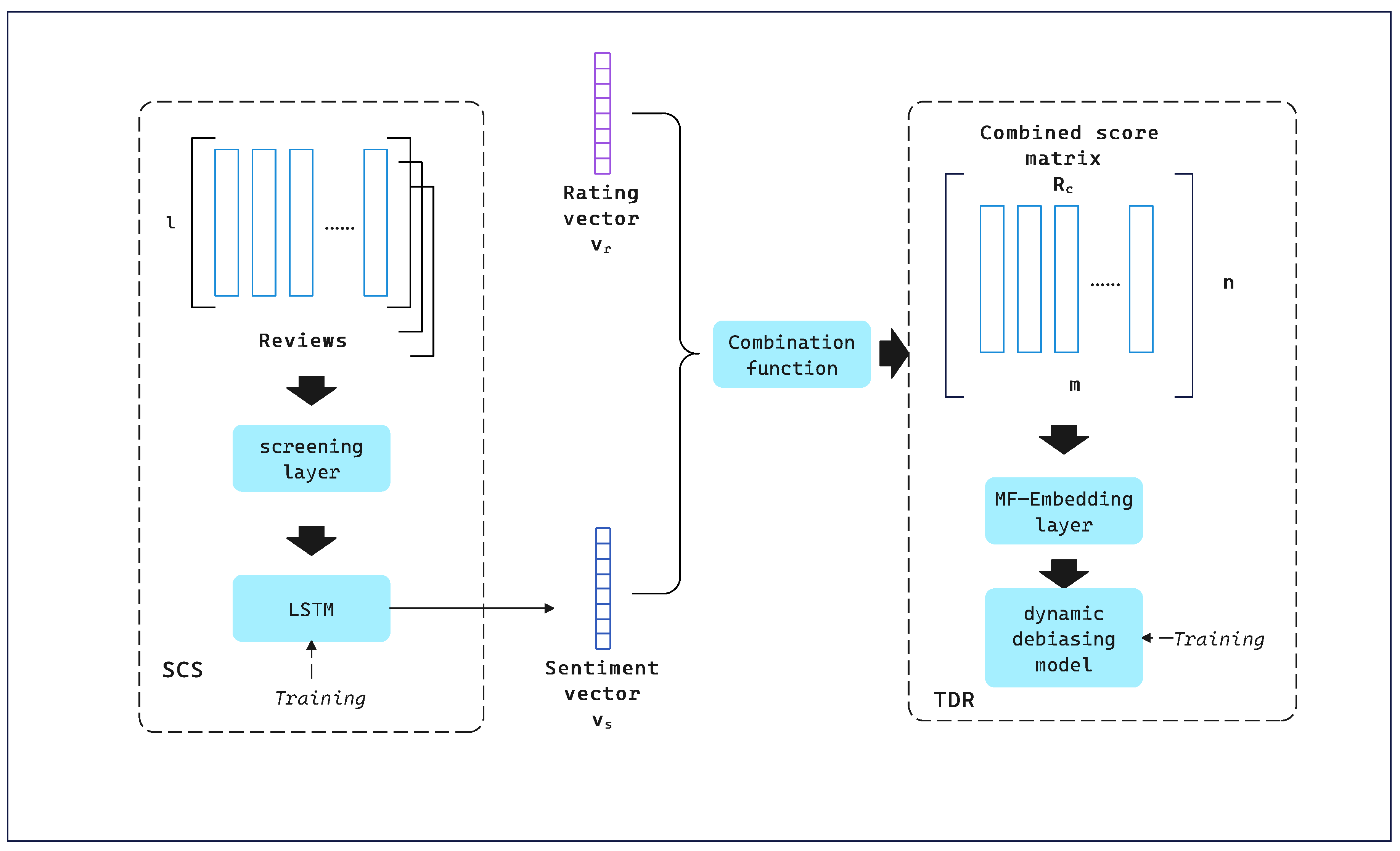
In this section,we focus on a framework for SCTD based on sentiment analysis and causality.SCTD consists of two modules:SCS and TDR.SCS is a convolutional neural network for sentiment analysis. The SCS output from user
U is a sentiment vector whose entries are the scores of each item in
U ’s review. At the same time, the columns of the user-item rating matrix are selected to form the rating vector
. Using the combinatorial function, an augmented rating matrix
is obtained, which we then provide to the TDR for accurate recommendation.The frame diagram for SCTD is shown in
Figure 1.
3.1. SCS
Unlike previous dichotomous sentiment analysis tasks, we have optimised the output of the sentiment score ratings to fit the scores, ranging from 0 to 5 to fit the corresponding score ratings.In our proposed recommender system, let U, I be the set of users and the set of items, respectively,
=
m,
=
n. The user-item matrix
consists of
m users, and
n items.
represents the evaluation of item
i by user
u, and
V represents the entire review text.The input to SCS is
V and the output is the set of vectors
.We propose that there are four hidden layers in the SCS model.The first layer is the embedding layer, which aims to convert user comments
V into a dense set of feature vectors. We arrange all the comments of user
into a matrix
. For each
, the embedding layer can be represented as:
Where
is equal to the number of items rated by user
u,
l represents the length of the review, and
k represents the latent dimension of the embedded word.Turning each word in a review into a
K-dimensional vector, the latent description of user
u’s reviews is as follows:
Where is an I-dimensional vector and the term of the inner word is a K-dimensional potential vector. represents u’s review of i. ⊙ represents the concatenation operator that combines these vectors into a description matrix .And then we input into the second layer, the convolution layer. We use attention theory to adjust different weights for each word of the review and each review of the review description matrix. Where g represents the K-dimensional embedding of each word.
and
represent the attention vector for each word in the review and the attention vector for each review in the review matrix. Next, we input the output vector obtained above into the convolution layer to extract contextual features between words. It can be expressed as:
Where,
and
are the weights of the filter function in the convolutional neural network.
is a nonlinear activation function. The third layer is the maximum pooling layer, which extracts the most important information from many contextual features. The max-pooling function is defined as follows:
The above vectors will be resolved to the final layer: the fully connected layer:
Where and are the weights in the fully connected neural network. can be a nonlinear activation function or a linear activation function.
Because we want to train the network with ratings rather than binary sentiments, we use softmax as the output function. The SCS process can be described as follows:
Where stands for .
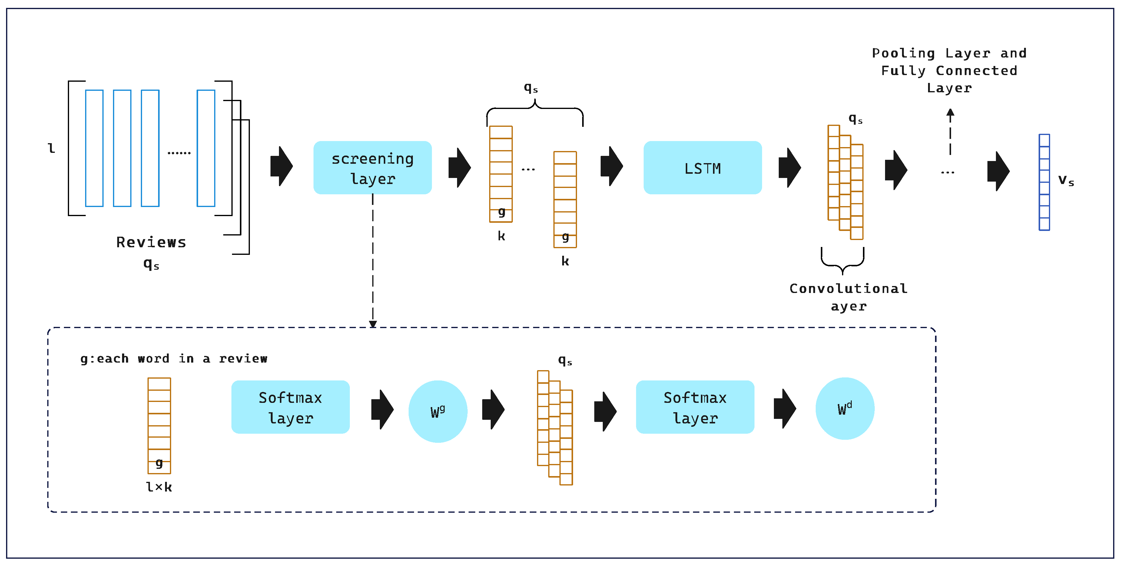
We use user ratings to train this convolutional neural network. Unlike traditional methods, we did not convert the scores in the training data (0-5) into six ranges of 0-1 for bi-affective analysis. Instead, we design the output of SCS into six classes, which can be treated as a regularization of the output layer. Our model naturally matches a user’s rating (from 0 to 5) with an sentiment score. Finally, we calculate the sentiment score vector
, whose entry is sentiment score
, with a range of (0-5).The specific flow of SCS is shown in
Figure 2.
3.2. Combination Function
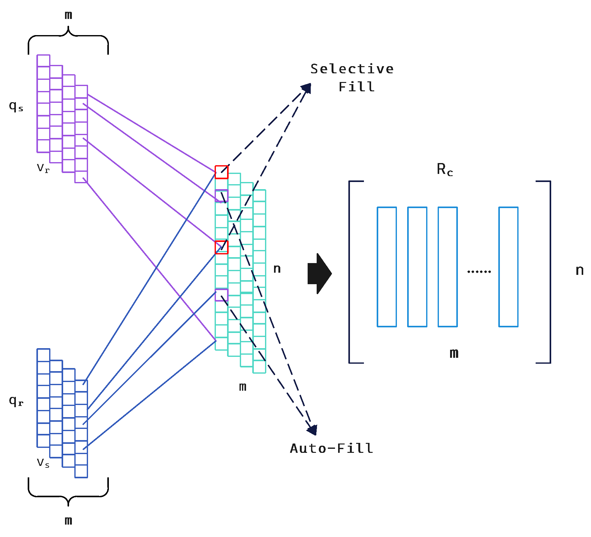
In this section, we introduce the combination function which captures the opinion bias of reviews on ratings and augments the original rating matrix.The specific flow of the combined function is shown in
Figure 3.
In the combination function, we make use of the sentiment vector
for each user in the sentiment rating module. we also extract each column from the user-item rating matrix
as a rating vector
. We then use a simple but efficient function to build a joint vector
with
and
:
where ⊕ is a combinatorial function of SCTD.
is an n-dimensional vector,
is a
-dimensional vector with entry
, and
is a
-dimensional vector with entry
, where
is equal to the number of the item evaluated by the user. In practice,
≥
. We assume that
=
.Whether we use review-based recommender system or rating-based recommender system alone, some important information of the other party is inaccessible, so it is difficult for us to solve the problem of data imbalance. Meanwhile, some users may make some useless reviews for some reasons (malicious reviews, hurried reviews, etc.). If a user rates an item and writes a review, we can compute the sentiment rating
from SCS and get the rating
from
r. The difference between
and
is exactly the opinion bias we want to detect,
. If
is too large, we treat the review as a bad review and delete it. If the user’s
is too large and too frequent, we treat it as a bad user and discard it. Basically, we want to enhance expressiveness through reviews and ratings while filtering out useless reviews. Thus the combinatorial function ⊕ can be generalised to the following three cases.
Auto-Fill : If user u only rates or reviews on item i, ⊕ will populate it with or .
Selective Fill : If user u rates and reviews on item i and does not discard it, then ⊕ will fill with a fixed weighted linear function .
Drop : If ≥µ, ⊕ reduces the user’s sentiment score for item i; if ≥, ⊕ drops user u as a bad user. , are predefined thresholds and is the number of deleted reviews.
According to the processing corresponding to the above situation, the enhanced rating matrix
is constructed, which is expressed by the formula, where
represents
:
3.3. TDR
Traditional debiased recommendation methods are based on static scenarios.
However,traditional recommendation methods with static bias are not unbiased for the current treatment of selection bias in dynamic scenarios.The current widely used debiasing method uses IPS estimation to correct the probability that a user will rate an item. It uses static propensity , which is the probability that user u observes a particular rating in any time period.
But this approach this ignores the dynamics of selection bias, i.e., these probabilities will vary
t in each time period, causing the static IPS estimator to become:
Items in collection
are recommended to users in collection
.Users have preferences with respect to items, which are generally modelled by a label
per user
and per item
.
is a set of time periods; we allow the user’s preferences
to change at different time periods
.As Eq.
shows,
refers to the static propensity, which refers to the probability that user
u observes a particular rating of item
i in any time period.In reality, user interaction data is very sparse, so it is unrealistic to have all users provide ratings for all items. In the Eq.
, the observation metrics matrix
indicates which ratings were recorded in the recorded interaction data and which ratings were recorded at that time period. When
it means that ratings of user
u for item
i in time period t have been recorded in the logged data, and if
it means that they are missing.Compared to the Eq.
, the conventional RS debiasing losses are as follows:
Where the function L can be chosen according to different RS evaluation metrics, if it is a common Mean Square Error (MSE) metric, the formula is as follows:
In the above we mentioned the plain recommendation loss function and the static IPS-based loss function, next we focus on the dynamic selection bias.We set the exact propensity
such that the dynamic selection bias can be fully corrected by applying the Eq.
to the evaluation of the predicted scores with reverse weighting:
Apply the Eq.
to the matrix factorization(MF) model. We refer to this method, which combines MF and time-dynamic debiasing methods, as TDR. Given an observed rating
from user
u on item
i at time
t,MF computes the predicted rating
as:
,where the
and
are embedding vectors of user
u and item
i, and
,
, and
are user, item and global offsets, respectively. Crucially,
is a time-dependent offset and models the impact of time in rating prediction.Under this model, the proposed TDR is optimised by minimising the loss of:
where
P,
Q and
B denote the embedding of all users, all items, and all offset items, respectively;
is the MSE loss function.
4. Experiments
4.1. Datasets
To validate the effectiveness of our model, we conducted extensive experiments on datasets from Amazon.com and Yelp’s RecSys. The Amazon and Yelp datasets are well known public recommendation datasets with textual information. However, both datasets are pre-filtered, so they cannot verify the robustness to imbalance and opinion bias. Therefore, we collect two real-world datasets from Taobao and Jingdong on our own as a supplement to validate our method. All datasets contain a rating range of 0 to 5. We use 5-fold cross-validation to partition the datasets, with 80% as the training set, 10% as the testing set, and 10% as the validation set. The details of the datasets are shown in
Table 1.
4.2. Baselines
The following is a description of the models compared in this paper:
- (1)
Static Average Item Rating (Avg): The average observed rating across all item-ages.
- (2)
Time-aware Average Item Rating (T-Avg): The average observed rating per item-age.
- (3)
Static matrix factorization (MF): A standard MF model that assumes selection bias is static.
- (4)
Time-aware matrix factorization (TMF) [16]: TMF captures the drift in popularity as items get older by adding an agedependent bias term.
- (5)
Time-aware tensor factorization (TTF) [17]: TTF extends MF by modelling the effect of item-age via element-wise multiplication.
- (6)
MF-StaticIPS: MF combined with static IPS methods.
- (7)
TMF-StaticIPS: TMF combined with static IPS methods.
- (8)
MF-DANCER: MF combined with dynamic IPS methods.
4.3. Experiment Results
The main results of our comparison are shown in
Table 2, from which we can easily observe that the event-based approach outperforms the static approach by a large margin. This shows that assuming a user preference is static when it is actually dynamic can seriously compromise method performance. Among them, SCTD is the best performing method, which starts from the data and establishes the sentiment score module, alleviating the problem of data sparsity and imbalance. Meanwhile, it combines IPS and MF based on dynamic scene time correlation, alleviating the influence of selection bias in many ways.
5. Conclusions
In this paper, we consider selection bias in dynamic scenarios and the impact of sentiment factors on bias. Based on the bias caused by sentiment factors, we built the SCS module for processing, which solves the problem of sentiment bias between review and ratings by filtering bad reviews through a screening layer, and then deriving the sentiment score matrix through a training layer. At the same time, We applied a debiased recommendation method based on time dynamic scenarios to process the enhanced rating matrix obtained from the previous optimization of the sentiment score module to mitigate the influence of selection bias.The experimental results on Amazon,Yelp and Taobao datasets showed that our approach outperforms these baselines in terms of valuation metrics by analogy with.
In future work, we should consider other aspects of time, such as seasonal effects and the difference between weekdays and days off, while the possibility of multi-modal debiasing of recommendation system can be investigated through problems related to sentiment bias.
Author Contributions
Conceptualization, F.Z.; methodology, F.Z.; software, F.Z.; validation, F.Z.; formal analysis, F.Z. and W.L.; investigation, F.Z.; resources, F.Z.; data curation, F.Z.; writing—original draft preparation, F.Z.; writing—review and editing, W.L.; visualization, F.Z.; supervision, X.Y.; project administration, W.L.; funding acquisition, X.Y. All authors have read and agreed to the published version of the manuscript.
Funding
This work was inspired by the National Social Science Foundation of China (NSFC) project ‘Research on Data Bias Identification and Governance Mechanisms Based on Digital Twins’, Project No. 22BTQ058.
Institutional Review Board Statement
Not aplicable.
Informed Consent Statement
Not aplicable.
Data Availability Statement
The data that support the findings of this study are available from the corresponding author upon reasonable request.
Acknowledgments
We are grateful to Hebei University for their cooperation and assistance.
Conflicts of Interest
The authors declare no conflicts of interest.The funders had no role in the design of the study; in the collection, analyses, or interpretation of data; in the writing of the manuscript; or in the decision to publish the results.
Abbreviations
The following abbreviations are used in this manuscript:
| IPS |
Inverse Propensity Scoring |
| MF |
Matrix Factorization |
| SCTD |
Sentiment Classification And Temporal Dynamic Debiased Recommendation Module |
| SCS |
Sentiment Classification Scoring Module |
| TDR |
Temporal Dynamic Debiased Recommendation Module |
| LSTM |
Long Short-Term Memory |
References
- Marlin, B.M.; Zemel, R.S. Collaborative prediction and ranking with non-random missing data. In Proceedings of the Proceedings of the third ACM conference on Recommender systems, 2009, pp. 5-12.
- Ovaisi, Z.; Ahsan, R.; Zhang, Y.; Vasilaky, K.; Zheleva, E. Correcting for selection bias in learning-to-rank systems. In Proceedings of the Proceedings of The Web Conference 2020, 2020, pp. 1863–1873. [Google Scholar]
- Pradel, B.; Usunier, N.; Gallinari, P. Ranking with non-random missing ratings: influence of popularity and positivity on evaluation metrics. In Proceedings of the Proceedings of the sixth ACM conference on Recommender systems, 2012, pp.147–154.
- Schnabel, T.; Swaminathan, A.; Singh, A.; Chandak, N.; Joachims, T. Recommendations as treatments: Debiasing learning and evaluation. In Proceedings of the international conference on machine learning. PMLR; 2016; pp. 1670–1679. [Google Scholar]
- Adamopoulos, P.; Tuzhilin, A. On over-specialization and concentration bias of recommendations: Probabilistic neighborhood selection in collaborative filtering systems. In Proceedings of the Proceedings of the 8th ACM Conference on Recommender systems, 2014, pp.153–160.
- Imbens, G.W.; Rubin, D.B. Causal inference in statistics, social, and biomedical sciences; Cambridge university press, 2015.
- Huang, J.; Oosterhuis, H.; De Rijke, M. It is different when items are older: Debiasing recommendations when selection bias and user preferences are dynamic. In Proceedings of the Proceedings of the fifteenth ACM international conference on web search and data mining, 2022, pp.381–389.
- Yang, X.; Guo, Y.; Liu, Y.; Steck, H. A survey of collaborative filtering based social recommender systems. Computer communications 2014, 41, 1–10. [Google Scholar] [CrossRef]
- Beel, J.; Gipp, B.; Langer, S.; Breitinger, C. Paper recommender systems: a literature survey. International Journal on Digital Libraries 2016, 17, 305–338. [Google Scholar] [CrossRef]
- Rubens, N.; Elahi, M.; Sugiyama, M.; Kaplan, D. Active learning in recommender systems. Recommender systems handbook.
- Zhang, F.; Yuan, N.J.; Lian, D.; Xie, X.; Ma, W.Y. Collaborative knowledge base embedding for recommender systems. In Proceedings of the Proceedings of the 22nd ACM SIGKDD international conference on knowledge discovery and data mining, 2016, pp.353–362.
- Panniello, U.; Tuzhilin, A.; Gorgoglione, M. Comparing context-aware recommender systems in terms of accuracy and diversity. User Modeling and User-Adapted Interaction 2014, 24, 35–65. [Google Scholar] [CrossRef]
- Champiri, Z.D.; Shahamiri, S.R.; Salim, S.S.B. A systematic review of scholar context-aware recommender systems. Expert Systems with Applications 2015, 42, 1743–1758. [Google Scholar] [CrossRef]
- Koren, Y. Collaborative filtering with temporal dynamics. In Proceedings of the Proceedings of the 15th ACM SIGKDD international conference on Knowledge discovery and data mining, 2009, pp.447–456.
- Xu, Y.; Yang, Y.; Han, J.; Wang, E.; Zhuang, F.; Yang, J.; Xiong, H. NeuO: Exploiting the sentimental bias between ratings and reviews with neural networks. Neural Networks 2019, 111, 77–88. [Google Scholar] [CrossRef] [PubMed]
- Koren, Y.; Rendle, S.; Bell, R. Advances in collaborative filtering. Recommender systems handbook.
- Rosenthal, S.; Farra, N.; Nakov, P. SemEval-2017 task 4: Sentiment analysis in Twitter. arXiv preprint arXiv:1912.00741, arXiv:1912.00741 2019.
- Han, J.; Zuo, W.; Liu, L.; Xu, Y.; Peng, T. Building text classifiers using positive, unlabeled and ‘outdated’examples. Concurrency and Computation: Practice and Experience 2016, 28, 3691–3706. [Google Scholar] [CrossRef]
- Liu, Q.; Wu, S.; Wang, L. Cot: Contextual operating tensor for context-aware recommender systems. In Proceedings of the Proceedings of the AAAI Conference on Artificial Intelligence, 2015, Vol.
|
Disclaimer/Publisher’s Note: The statements, opinions and data contained in all publications are solely those of the individual author(s) and contributor(s) and not of MDPI and/or the editor(s). MDPI and/or the editor(s) disclaim responsibility for any injury to people or property resulting from any ideas, methods, instructions or products referred to in the content. |
© 2025 by the authors. Licensee MDPI, Basel, Switzerland. This article is an open access article distributed under the terms and conditions of the Creative Commons Attribution (CC BY) license (https://creativecommons.org/licenses/by/4.0/).