
Submitted:
04 January 2025
Posted:
06 January 2025
You are already at the latest version
Abstract
Transportation of hazardous chemicals is a critical component of chemical logistics, with unique properties such as flammability, explosiveness, and corrosiveness posing significant risks of catastrophic accidents. While the current literature has focused on reducing the overall risk within hazardous materials transportation systems, it has paid less attention to the equitable distribution of risks across regions from a public health perspective. Furthermore, there is a scarcity of research on the optimization of hazardous material transportation routes that consider risk equity in the context of fluctuating population densities and wind speeds. This article considers the impact area of hazardous chemical accidents under various wind speed conditions. It then establishes a time-varying risk assessment function that considers changes in population density over time. The Gini coefficient is employed to quantify the disparity in risks among different routes. Building on this foundation, we propose a novel time-varying route optimization model for hazardous materials transportation that incorporates risk equity considerations. Secondly, we design an improved genetic algorithm based on the ε-constraint method to solve the proposed model efficiently. Finally, the research methodology is applied to a realistic transportation network in Shanghai, providing a case study that illustrates the application of the model. The study also examines the temporal distribution of risk equity, offering practical and feasible insights into the dynamics of risk allocation in practical scenarios.
Keywords:
hazardous materials transportation
; time-varying
; risk equity
; bi-objective optimization
; genetic algorithm
1. Introduction
The advancement of Industry 4.0 has conspicuously enhanced productivity of the chemical industry which in tandem, has led to an amplified need for the transportation of hazardous materials. Road transportation is the most common mode of transportation due to its economy and flexibility [1]. Data indicate that in excess of one billion tons of hazardous commodities are conveyed via road annually within China, accounting for more than 60% of China’s total hazardous materials freight. Due to the unique nature of hazardous chemicals such as flammable, explosive, or corrosive, accidents during road transportation often cause serious consequences, extending to disastrous ramifications. A case in point was the train derailment event in the state of Ohio, USA, on February 3, 2023, which culminated in the atmospheric liberation of toxic substances, including vinyl chloride, engendering persistent adverse effects on local health and ecology.
Currently, the focus of hazardous materials transportation research is primarily on developing methods to reduce the overall risk within the transportation system. However, the literature has shown a relative dearth of research concerning the equitable distribution of risk across different societal segments—a concept known as risk equity. This oversight is particularly pronounced in the context of models that consider the temporal and spatial variances in risk, which are paramount for a comprehensive understanding of Hazmat transportation dynamics. However, with the evolution of society, there is an escalating public emphasis on equity. The concept of equity has been progressively incorporated across various domains of scholarly inquiry [2] articulated the notion of “risk equity” by conceptualizing it as the maximized disparity in the levels of risk among a collective of individuals. When planning the transportation of hazardous materials, it is insufficient to solely focus on the minimization of accident risks. Attention should also be given to the disparities in risk across various population centers and transportation routes.
Compared to regular industrial activities, the transportation of hazardous goods exhibits substantial “dynamic” characteristics [3]. The parameters of transportation networks vary considerably within a day, with factors such as population density, traffic flow density, and wind speed evolving according to different times. Accordingly, the temporal variation and dynamism of networks should be considered in the portrayal of risk equity functions and risk assessment. At the same time, wind speed is a crucial factor in the risk assessment of road transport of dangerous goods, because it directly affects the diffusion simulation of gas leakage, ventilation effect, driving conditions and surrounding environment. Specifically, the wind speed determines the diffusion mode and speed in the air after gas leakage, and different wind speed conditions will produce different diffusion effects, thus affecting the safety of a specific area. At the same time, the wind speed will also affect the potential impact of harmful gases on the surrounding residential areas and buildings. When the wind speed is high, it may accelerate the diffusion of the gas and increase the harm to the environment. Therefore, the combined action of these factors makes the transportation risk of hazardous chemicals show obvious dynamic change characteristics, and put forward higher requirements for transportation safety management. The risk assessment and management requires considering the combined impact of these factors and taking appropriate preventive and control measures to secure the transportation process.
In this study, based on wind speed conditions, the affected area is divided into different sub-regions. Under windy conditions, according to the Emergency Response Planning Guidelines (ERPG) isopleth curves, the Potential Impact Zone (PIZ) is divided into three sub-regions, which are represented by a simplified elliptical model. Under light wind and calm conditions, the behavior of pollutant diffusion is not significant in the horizontal direction, but it is the same as in windy conditions in the vertical direction. Therefore, this paper assumes that under light wind and calm conditions, the gas diffusion does not exhibit obvious directionality in the horizontal direction, but is the same as in windy conditions in the vertical direction. A simplified calculation method is provided based on the Gaussian plume model. Meanwhile, taking into account the differences in regional emergency response capabilities. Considering both spatial and temporal factors, the risk assessment and risk equity functions are comprehensively evaluated.
The contributions of this paper are as follows. Firstly, it presents a model for dynamic risk equity and risk appraisal, enabling the comprehensive utilization of both real-time and static data to analyze the peril associated with hazardous chemical transportation in a widely scientific and rational manner. Secondly, this paper constructs a route optimization model for hazardous materials transportation considering risk equity under time-varying conditions, further enriches the network optimization model method, and explores the law of the distribution of risk equity over time to make up for the lack of research. Finally, the results of this study can assist traffic authorities in devising more effective strategies while offering science-based methods for government and hazardous goods transportation entities.
2. Literature Review
2.1. Risk Assessment
The risk model provided by [4,5] is widely used to support safety-critical decision-making for the transportation of hazardous goods [6,7,8]. This simplified risk model is based on a combined assessment of the expected accident frequency and the consequences of the impact on the population. Hazard circles are used to estimate the consequences, defining unit section risk and marginal risk. On this basis, Jabbarzadeh (2021) incorporates risk variability into the risk assessment function [9]; provides a real-time risk quantification tool for tanker trucks and Tianming (2022) proposes a “zone of potential impact” based on a Gaussian plume model “ model to describe the area of influence of a toxic gas leak and uses point of interest (POI) data to identify critical targets [10].
The impact of wind speed on transportation risk assessment is specific in terms of diffusion effects and accident consequences. Tan (2021) conducted tests with different wind speeds and found a negative correlation between wind speed and exposure to vehicle emissions in the area, as the slower the wind speed, the lower the degree of pollutant diffusion in the air [11]. Zhang (2020) established a simulation model of the gas pipeline in the comprehensive pipe gallery and simulated the situation of gas leakage and diffusion at different ventilation speeds [12]. The results indicated that the faster the ventilation speed, the lower the gas concentration in the diffusion area. Wang Haiyan et al. (2012) set up typical scenarios of atmospheric diffusion based on wind direction, wind speed, and other meteorological data, and improved the Gaussian plume model to calculate the diffusion of pollutants at affected points [13]. Wang Yong et al. (2020) studied the negative relationship between PM2.5 concentration and wind speed through regression analysis [14]. These studies demonstrate that wind speed is a key factor affecting the diffusion of pollutants and risk assessment, and it is crucial for developing effective risk management and mitigation measures.
2.2. Optimization of Hazardous Materials Transportation Routes Under Time-Varying Conditions
Zandieh et al. (2023) proposed and managed a multi-objective time-varying hazmat route problem by modeling the effect of time on population density [15]. Ke (2022) constructed two mixed-integer planning models based on population dynamics and risk assessment to manage a reliable emergency response system [16]. Androutsopoulos et al. (2012) developed a bi-objective vehicular route model on time-varying networks to minimize the transportation cost and total risk [17]. Desai et al. (2013) investigated the population density-varying hazardous goods route problem on a stochastic dynamic network over the time-varying hazardous materials transportation route problem [18]. Chious (2020) proposed a resilience-based time-varying route planning approach to optimize hazardous materials transportation routes and enhance the resilience of the road network by dynamically adapting the signal control [19].
2.3. Risk Equity
There are two main ways to achieve risk equity in hazardous materials transportation route selection: to directly control the risk differences on different populations, regions, or road sections by setting thresholds, i.e., setting risk equity constraints in the model. In order to distribute the risk equitably, Fontaine et al. (2020) proposed a new population-based definition of risk, which evaluates the risk of the population of any given region in its intermodal network [20]. Different objective functions are proposed to balance the risk and achieve a better population risk distribution. Bhavsar (2022) uses subsidies to mitigate the risk and ensure a more equitable distribution of risk [21]. Hosseini and Verma (2021) set risk thresholds for transit stations and track arcs, respectively, to achieve the goal of risk equity across the railway network [22]. Another approach is to use minimizing the maximum risk or minimizing the risk difference, i.e., setting the risk equity objective function in the model. Taslimi et al. (2017) aim to minimize the maximum total area risk in a two-tier planning problem, thus reflecting the risk equity property in the optimization results [23]. Ke et al. (2020) achieve the objective of minimizing the maximum total area risk in a two-tier charging strategy problem by minimizing the maximum link risk, making the spatial distribution of risk more uniform [24].
In summarization research primarily emphasizes aggregate network risk and transportation costs. However, societal advancements underscore the importance of equitable risk distribution alongside these traditional objectives. Scholars have recognized this shift and incorporated various methodologies to quantify risk equity in their models. Nevertheless, a notable gap exists in dynamically measuring risk equity, particularly in accounting for time-variable conditions such as changes in wind speed and the evolving impact of emergency response on accident consequences.
This paper introduces a fresh perspective on risk compensation costs, establishing a discrete function to delineate the time-sensitive risk equity and investigating temporal fluctuations in risk equity distribution. Extending beyond the conventional dual-objective model of risk and cost, this study introduces a novel objective of risk compensation costs. It specifically targets segments exceeding the mean risk of the pathway to ensure equitable risk distribution among transportation segments. The research offers strategic recommendations for government and transportation authorities to enhance both equity and safety within the hazardous materials transportation network.
3. Optimization Model
3.1. Description of the Problem
Given a hazardous material transportation network G = (U, V) consisting of a set of nodes N and a set of road segments V . Nodes i, j ϵ N and road segments (i, j) ϵ V. Now, hazardous chemicals need to be transported from the starting point O to the ending point D (O, D ∈ N). In this paper, based on the traditional multi-objective function of risk and cost and considering the public’s fairness claim, the Gini coefficient is used to reflect the difference between the risks borne by each route, which is quantified as the risk equity objective. In addition, the population density, traffic conditions, wind speed, etc. of each road segment in a day will change with time. Therefore, in order to better explore the law of risk equity over time, this paper adopts the discrete time-varying function to describe the time-varying characteristics of dangerous goods transportation, divides the 24 hours a day into 24 time periods, and constructs the optimization model of dangerous goods transportation routes on the time-varying network considering risk equity.
3.2. Model Assumptions and Parameters
- Assuming that a tank vehicle transporting toxic gases stops moving after a spillage
- Assuming that the hazardous material leaks immediately after the vehicle overturns on the road, the vehicle is considered a point source of risk, and the leaked hazardous material is airborne.
- The source strength of the leakage source and the stability of the wind speed around the leakage source point.
- Hazardous goods transportation vehicles have the same probability of being involved in an accident on each unit length of road.
- Hazardous materials have the same probability of leakage under accident conditions in transportation vehicles.
- Assuming that the government and regulatory bodies can provide risk compensation to the public.

Table 1.
Model sets and indices.
| set(mathematics) | |
| N | A collection of nodes in a hazardous materials transportation network whose elements are denoted by i or j |
| V | A collection of road segments in a hazardous materials transportation network with elements denoted by (i, j) |
| set(mathematics) | |
| Gini coefficient | |
| Risks of transporting category m hazardous chemicals at time t | |
| Average risk on the road network for the transportation of hazardous chemicals | |
| ω | Unit reimbursement cost |
| Wind speed at section (i,j) at time t | |
| Probability of hazardous chemical transportation spillage accident when the hazardous chemical transportation vehicle is transported on a road section | |
| βLimit value for the concentration of hazardous materials in the zone, mg/m3 | |
| Q | The intensity of the point source, i.e., a mass of gas emitted from the point source per unit time, mg/s |
| “Potential impact area” at time t, i.e., the area of exposure of the population affected by the accident | |
| Population exposure radius of the leakage source at point (i,j) of the road section at time t | |
| Population lethality in the event of a spillage of m hazardous chemicals transported in mode h | |
| Consequences of a Hazardous Chemical Spill at time t | |
| Vehicle density on road section (i, j) at time t in vehicles/km | |
| Exposure costs per unit of population | |
| Cost per unit distance traveled by a hazardous goods vehicle, in $/km | |
| Population density between node i and node j | |
| Movement distance from node i to node j | |
| O | Starting point for the transportation of hazardous goods |
| D | Starting point for the transportation of hazardous goods |
| variant | |
| 0-1 variable, one if a hazardous materials vehicle k travels from node i to j. Otherwise, the result is 0 |
3.3. Model Construction
3.3.1. Potential Impact Zone
In this paper, the space that may be affected to some extent by hazardous phenomena is considered the “potential impact zone” (PIZ).
Transient leakage from a fixed point source, continuous leakage from a fixed point source, and continuous leakage from a mobile point source are the three main scenarios of tanker truck leakage accidents, accounting for 4%, 95%, and 1%, respectively (Zhang et al., 2015). As the most common scenario, continuous leakage from a fixed point source was chosen as the hypothetical scenario for hazardous chemical accidents in this study. The Gaussian smoke and rain model is widely used for modeling gas diffusion from continuous leakage from a fixed point source due to its good agreement with experimental results and simple calculation method, which is formulated [25] as follows (Zhao et al., 2014):
The Gaussian model diffusion coordinate system shown in the Figure 1, with the leakage source as the coordinate origin, where the x axis is in the same direction as the direction of the wind, the y axis represents the lateral distance, while the z axis indicates the vertical height.
Where C(x, y, z, t) denotes the concentration of hazardous chemicals at any location at time t section (i, j), mg/m3; Q represents the intensity of the point source, i.e., the mass of gas emitted from the point source per unit of time, mg/s; u-mean wind speed, m/s; and σy and σz are the horizontal diffusion parameter and vertical diffusion parameter, respectively, according to the study [26] (Zhang et al., 2020), which can be determined from atmospheric stability and coordinates x and y. Atmospheric stability is determined by cloudiness, solar radiation, and average wind speed. All of the above weather-related parameters can be obtained through the API. h is the effective height of the point source. This study manually sets the parameters as static parameters for ease of calculation.
When y = 0 and z = 0, Eq.1 can be converted to Eq.2 to calculate the gas concentration along the centerline of the ground:
The gas concentration classification criteria chosen for this paper refer to the Emergency Response Planning Guidelines (ERPG), and according to the AEGL criteria, the concentration profiles such as ERPG-1, ERPG-2, and ERPG-3 divide the PIZ into three sub-areas, denoted asβ=1,2,3. Targets in the different subregions between the concentration curves are considered to be exposed to toxic gases to varying degrees.
In this model, and depend mainly on the atmospheric stability parameters , where , Set as β Limit value of the concentration of hazardous materials in the area, mg/m3. The population exposure radius of the leakage source at point (i,j) of the road section at time t is shown in Equation (3). The area of the accident-affected population exposure along the section (i,j) of the road section is shown in Figure 2 and Figure 3, and the equations are as follows:
According to the study [27] (Huang et al.,2021), the Gaussian diffusion model needs to consider two types of wind conditions: one is wind (u>1.5m/s); the other is light air (0.5m/s<u≤1.5m/s) and no wind (u≤0.5m/s).
When the wind (u >1.5 m/s), according to Equation (2), The original shape of the Gaussian smoke model is the concentration curve drawn is complex, and some studies [28,29] (Pan et al, 2000; Xia et al. 2014a) have simplified it to an ellipse.
As shown in the figure, assuming that the wind direction of the toxic gas leakage scenario is θ= 60°, three elliptical ERPG isoconcentration profiles constitute the impact area. Considering the urgency and necessity of ERPG-3 concentration to evacuate people and that a single elongated elliptical impact area may underestimate the actual impact range of a hazardous chemical spill, the elliptical impact area can be expanded into a sector.
In modeling gas diffusion under light air (0.5m/s<u≤1.5m/s) and no wind (u≤0.5m/s) conditions, the following assumptions are made: the behavior of gas diffusion has no apparent direction in the horizontal direction but is the same in the vertical direction as in the wind condition. Therefore, the final shape of the PIZ under light wind and no wind conditions is three concentric circles, as shown in Figure 3
The corresponding area formula is shown in Equation (5):
3.3.2. Consequences of the Accident
The probability of lethality of the exposed population is related to the type of toxic gas in the area, its concentration, and exposure time, and based on the Gaussian gas diffusion model in the previous section, the toxic concentration can be calculated for any location. According to the formula, the probability of lethality in theβ zone .
A, B, and n denote constants of the toxicant; C denotes the concentration of the exposed toxicant; and t is the exposure time. Therefore, the total accident consequences of population exposure in the time-varying conditions of road section (i, j) can be defined as in Eq.7 :
Regarding the assessment of time-varying risk , this paper will be based on the traditional risk model, risk equals the probability of an accident multiplied by the consequences arising from an accident. The risk assessment model for hazardous materials transportation at moment t can be defined as in Eq.8:
3.3.3. Time-Varying Risk Equity Function
The Gini coefficient is used to reflect the difference between the risks borne by each route, which is quantified as the risk equity objective. indicates the number of road network sections. It can be expressed as in Eq.9:
3.3.4. Time Varying Route Optimization Considering Risk Equity Model
Objective function
s.t.
The objective function (10) minimizes the transportation risk. The objective function (11) reflects the risk equity. Constraint (12) is a flow conservation constraint, i.e., the net outflow at the starting point is unit 1, the net outflow at the endpoint is -1, and the net outflow at each endpoint in between is 0. This ensures that the direction of vehicle transportation is from the starting point to the endpoint. Constraint (13) prevents the occurrence of a high risk value that is masked by the general situation where the total transport risk for most sections is spread around the average of the total transport risk for all sections. Constraint (14) limits the transportation cost. The total transportation cost in this paper consists of two parts: the transportation cost of the planned road section and the population exposure cost after an accident. The transportation cost of the road section (i,j) is , and is the cost per unit of distance traveled by a hazardous material vehicle, unit: yuan/km. Constraint (15) is the range of values for the decision variables.
3.4. Model Transformation and Solution
To handle the objectives in our model, we employ the augmented-constraint method [30] proposed by Mavrotas (2009). Regarded as an exact approach, it is able to produce a global set of Pareto frontier solutions, where the density of solutions can be easily adjusted. This is because the augmented version has embedded the optimization process within the other objective functions, which are transferred to the problem constraints [31] (Mavrotas and Florios, 2013). Furthermore, unlike many other popular multi-objective methods, the AECM frees the decision-maker from needing to determine about the weights of the objective functions, which eliminates the need to scale them over each other. Application of the AECM results in the following new terms in which one of the objective functions, here z1, remains as the primary objective function of the problem. However, the other objective function z2 is transferred into the problem constraints section as a new constraint with an enforcing upper bound as follows:
Thus, the multi-objective problem is transformed as follows:
3.5. The NSGA-II Solution Algorithm
In this chapter on the risk fair path optimization model, we mainly focus on two tasks: one is to reduce the overall risk of hazardous chemicals transportation; the other is to reduce the risk gap. The trade-off between the two is critical because we must strike a balance between these two requirements in our search for the optimal solution. Compared with GA, NSGA-II algorithm is based on the dominant relationship of the solution in the feasible solution space, which can better maintain the population diversity in solving the multi-target problem, has better convergence performance, and provides the choice [32] for trade-off between multiple targets. NSGA-II algorithm has the characteristics of fast solution, good convergence, and robust, therefore, NSGA-II algorithm is widely used [33,34] in similar dual-objective optimization studies.
Given the specific features of the model discussed here, we investigated genetic factors and chromosome repair functions that are particularly relevant to this model. A NSGA-II algorithm is designed for the model. The flow of genetic algorithm is shown in the Figure 4 below. In order to further consider the carrier cost limit and risk level limit, to improve the traditional NSGA-II algorithm, designed in the algorithm consideration for transportation cost constraints and risk limit of population repair steps, does not meet the two constraints of individuals will be eliminated in advance and generate new individuals, in order to improve the applicability of the algorithm:
initialization: set for transportation network parameters, including network nodes, network link, population density, wind speed, etc., and according to the Dijkstra algorithm for transportation requirements search for transportation feasible path and number, and set the size of the size of the population, the number of iteration, cross operator and variation operator.
Chromosomal coding: using 0-1 encoding, to search for a set of transportation routes that meet the requirements for the transportation of hazardous chemicals through path search algorithms. The set of hazardous chemical transportation routes is then encoded, with the decimal value of this encoding representing the number of the selected set of hazardous chemical transportation routes.
Initialized population: the initial population is randomly generated according to the set parameters and chromosomal coding rules.
Repair population: determine whether each individual meets other constraints related to transportation cost and risk. If not, the individual will be randomly generated to finally ensure that all individuals of the whole population meet the constraints.
Fitness Evaluation: Assess the fitness of each individual within the population. The total risk and risk equity target of hazardous chemical transportation are calculated for each individual within the population.
Fast Non-dominated Sorting: individuals are ranked to different Pareto levels according to the fitness value of individuals to determine the dominance relationship between individuals.
Crowding distance calculation: at each Pareto level, according to the target function value size, the boundary solution assigned infinite distance value, and according to the normalized difference of the intermediate solution, calculate the total crowding distance value of each solution, and consider the fitness and diversity in the selection operation.
Selection: Select individuals for reproduction based on their fitness, with a higher probability of selection for fitter individuals.
Crossover: Perform crossover on selected individuals to produce offspring, combining the genetic traits of the parents.
Mutation: Apply mutation to the offspring with a low probability, introducing genetic variation into the population.
Population Update: Form a new generation of the population based on fitness and selection strategies.
Termination Check: If the termination condition is met (such as reaching the maximum number of iterations or achieving a satisfactory fitness threshold), the algorithm halts and outputs the best solution found; otherwise, return to step 4 for further evolution.
4. Case Study
4.1. Example Background
According to the 2022 Shanghai Statistical Yearbook, there are 16 administrative districts in Shanghai, with a total area of 6,340.50 square kilometers, a resident population of 24,883,500 people, and an average population density of 3,925 people per square kilometer. The mileage of Shanghai’s road transportation in 2022 was 12,917 kilometers, of which the length of the motorway was 845 kilometers. The cargo volume transported in 2022 was 139,226,000 tons, and the kilometer freight was 460,510,000 tons. The volume of freight transportation in Shanghai is 139,226,000 tons, of which the volume of km freight transportation is 460,510,000 tons. This chapter is based on the road transportation network of Shanghai, and the software ArcMap is used to construct the road transportation network of hazardous chemicals in Shanghai, as shown in the Figure 5:
4.2. Example Data
It is assumed that the transported cargo, liquid ammonia, a hazardous chemical, is a toxic gas of category 2.3. The atmospheric stability class is D (neutral), and the diffusion parameters are as follows, according to the technical method for setting local air pollutant emission standards (GB/T3840-91).
Table 2.
Coefficient values for diffusion parameter expressions (GB/T 3840-91).
| Downwind distance m parametric |
1~1000 | 1000~10000 | >10000 |
|---|---|---|---|
| 0.929418 | 0.888723 | 0.888723 | |
| 0.110726 | 0.146669 | 0.146669 | |
| 0.826212 | 0.632023 | 0.55536 | |
| 0.104634 | 0.400167 | 0.810763 |
The American Industrial Hygiene Association (AIHA) has developed ERPG concentration thresholds that indicate the concentration of gas, vapor, or fumes acceptable for people to be continuously exposed to for 1 to 24 hours in an emergency situation and to perform the assigned tasks. The concentration thresholds and hazards for the different classes of liquid ammonia are shown in the table below.
Table 3.
Liquid Ammonia Toxicity Hazard Area Classification (AIHA).
| ERPG rating | ERPG_1 | ERPG_2 | ERPG_3 |
|---|---|---|---|
| Concentration (ppm) | 25 | 150 | 1500 |
| threaten | cause irritation | permanent damage | lethal |
This paper constructs the hazardous chemical transportation network by Songjiang District, Bao Shan District, Jinshan District, Pudong New District, Feng Xian District, Jiading District, Minhang District, Qing Pu District, Pu Tuo District, and the following is the data of each road section.
Table 4.
Road section data (Shanghai Meteorological Bureau &https://data.sh.gov.cn/).
Table 4.
Road section data (Shanghai Meteorological Bureau &https://data.sh.gov.cn/).
| Roads | Length (km) |
Wind speed (m/s) | Population density (persons/km2) | Main areas of transit |
|---|---|---|---|---|
| (3,5) | 10 | 2.19 | 7210 | Ming hang |
| (1,3) | 10 | 2.19 | 7210 | |
| (2,5) | 1 | 2.19 | 7210 | |
| (5,6) | 11 | 2.19 | 7210 | |
| (2,6) | 9 | 2.19 | 7210 | |
| (3,20) | 10 | 2.19 | 7210 | |
| (21,20) | 7 | 2.19 | 7210 | |
| (6,7) | 16 | 2.73 | 1669 | Feng Xian district |
| (7,27) | 31 | 2.73 | 1669 | |
| (7,8) | 14 | 2.73 | 1669 | |
| (8,9) | 8 | 2.73 | 1669 | |
| (2,9) | 11 | 2.73 | 1669 | |
| (9,11) | 9 | 2.73 | 1669 | |
| (1,9) | 16 | 2.73 | 1669 | |
| (10,11) | 6 | 2.75 | 1391 | Jinshan suburban district |
| (10,17) | 24 | 2.75 | 1391 | |
| (10,14) | 12 | 2.75 | 1391 | |
| (11,14) | 13 | 2.75 | 1391 | |
| (11,12) | 15 | 2.75 | 1391 | |
| (8,12) | 1 | 2.75 | 1391 | |
| (12,13) | 6 | 2.75 | 1391 | |
| (13,14) | 6 | 2.75 | 1391 | |
| (14,15) | 8 | 2.75 | 1391 | |
| (15,17) | 16 | 2.75 | 1391 | |
| (16,17) | 13 | 2.77 | 3201 | Song Jiang suburban district |
| (4,16) | 13 | 2.77 | 3201 | |
| (10,16) | 19 | 2.77 | 3201 | |
| (4,19) | 15 | 2.77 | 3201 | |
| (3,4) | 15 | 2.77 | 3201 | |
| (1,10) | 20 | 2.77 | 3201 | |
| (16,18) | 20 | 1.93 | 1929 | Qing Pu suburban district |
| (18,26) | 27 | 1.93 | 1929 | |
| (18,19) | 30 | 1.93 | 1929 | |
| (19,26) | 15 | 1.93 | 1929 | |
| (25,26) | 13 | 1.93 | 1929 | |
| (21,26) | 17 | 1.93 | 1929 | |
| (24,25) | 17 | 2.31 | 3996 | Jiading district |
| (22,25) | 22 | 2.31 | 3996 | |
| (21,28) | 17 | 1.23 | 22681 | Pu Tuo District |
| (22,24) | 16 | 2.36 | 8303 | Bao Shang district |
| (23,24) | 13 | 2.36 | 8303 | |
| (22,35) | 10 | 2.36 | 8303 | |
| (22,28) | 8 | 2.36 | 8303 | |
| (23,35) | 11 | 2.36 | 8303 | |
| (28,35) | 8 | 2.36 | 8303 | |
| (34,35) | 15 | 1.57 | 4765 | Pudong New District |
| (29,34) | 9 | 1.57 | 4765 | |
| (29,30) | 8 | 1.57 | 4765 | |
| (28,29) | 18 | 1.57 | 4765 | |
| (20,29) | 26 | 1.57 | 4765 | |
| (30,34) | 17 | 1.57 | 4765 | |
| (33,34) | 17 | 1.57 | 4765 | |
| (5,30) | 22 | 1.57 | 4765 | |
| (30,33) | 11 | 1.57 | 4765 | |
| (30,31) | 12 | 1.57 | 4765 | |
| (31,33) | 14 | 1.57 | 4765 | |
| (32,33) | 30 | 1.57 | 4765 | |
| (6,31) | 19 | 1.57 | 4765 | |
| (31,32) | 22 | 1.57 | 4765 | |
| (27,32) | 8 | 1.57 | 4765 |
4.3. Analysis of Result
4.3.1. Comparison of Route with and Without Risk Equity
According to the results of the Python genetic algorithm, assuming that a hazardous material transportation vehicle starts from node 24 and terminates at node 12, and 4-3 show the results of two transportation routes with and without risk equity, when the objective is to consider only the transportation risk and cost, the transportation route is 24-22-35-28-29-34-30-5-2-9-8-12. When risk equity is included in the objective, the optimal route is 24-22-35-28-29-30-33-31-6-7-8-12. Obviously, the hazardous material transportation route under the consideration of risk equity would deviate from the urban area, away from the population center and the road with high traffic density.
An increase in the risk compensation objective, which incentivizes the selection of longer but less risky alternative routes for hazardous goods tankers, could be used as a tool to promote a fairer distribution of hazardous goods risk on the rail network and, in general, a reduction in the total risk on the network. This finding has important guiding significance for the decision of hazardous chemical transportation. Policy makers should fully consider the risk equity factor when formulating transportation strategies, so as to achieve safer and more efficient transportation of hazardous chemicals.
4.3.2. Risk Equity and Aggregate Risk Change over Time
At a wind speed of 0.3 m/s, with node 24 as the starting point and node 12 as the endpoint for transporting hazardous chemicals, the optimal routes for each time period and the corresponding risk compensation coefficient values are shown in Table 5 below.
The route map for different time segments is shown in the Figure 7 below:
Temporal changes significantly affect population density. For instance, daily needs such as education and healthcare lead to higher concentrations of people in public spaces like schools and hospitals during the day. Conversely, residential areas see increased density during nighttime due to sleep and rest. Furthermore, research indicates that traffic risk exhibits distinct patterns over time, with peak traffic periods in the morning and evening when population and traffic density are higher, leading to a significant increase in traffic risk, peaking between [17,18]. This finding aligns closely with real-world observations, as during rush hours, there is a surge in travel activities, resulting in a higher number of vehicles and pedestrians on the roads. The increased population density amplifies the consequences of accidents and exacerbates traffic congestion, thereby raising the likelihood of accidents.
The risk Gini coefficient is susceptible to time change; the overall curve posture is very different from the value at risk, but the peak period is consistent with the value at risk [17,18]. This means that in the period of high risk, risk equity is more prominent. For example, in the morning and evening rush hours, not only the total risk is higher, but also the distribution of risk between different sections is more unbalanced. This may be because the main roads in some cities in the morning and evening rush hours bear more total traffic flow, while other sections have relatively low flow, exacerbating the uneven risk distribution. Moreover, different routes may have the same risk compensation value. This discovery provides us with more options and flexibility when optimizing transportation routes, allowing us to choose the most suitable route based on other factors, such as transportation costs and time, even when the risk equity is the same.
4.3.3. Wind Speed
The consequences of accidents in each type of hazardous area are further calculated, taking the northeast wind direction as an example, t time. The consequences of road transportation leakage accidents on each section of the road are shown in Table 6.
Analysis of the data in the table above shows that the greater the wind speed, the longer its diffusion radius and the larger the affected area. At the same time, the wind speed is inversely proportional to the accident consequences, that is, the higher the wind speed of the road section at time t, the less obvious the corresponding accident consequences. This is because of the dilution of dangerous goods. If it is assumed that the diffusion time of dangerous goods is not considered and the total amount of dangerous goods leaked is fixed, the higher the wind speed, the faster the diffusion of dangerous goods will be, which will lead to the dilution of dangerous goods. Then, as the concentration of dangerous goods (referring to AEGL standard) is set in advance in this paper, the dilution of dangerous goods will reduce the influence range of ERPG-3 when it reaches the prescribed concen3tration, and reduce the size of the area with high fatality rate, thus leading to the corresponding accident consequences becoming smaller. Therefore, in practice, governments and businesses should consider the effects of wind speed to reduce the consequences of any potentially catastrophic population exposure accidents.
Wind speed is a key factor affecting the dispersion of hazardous materials; the higher the wind speed, the broader the dispersion range. High wind speeds help to rapidly dilute the concentration of hazardous materials, increasing the affected area but reducing the consequences of an accident. To delve into the impact of wind speed on the risk of hazardous chemical transportation, we adjusted different wind speed parameters and obtained the Gini coefficients corresponding to the transportation of hazardous chemical goods under various wind speeds, as shown in Figure 4.8. The research results indicate that there is a complex relationship between the Gini coefficient and wind speed. At low wind speeds, the Gini coefficient gradually increases with the increase of wind speed, suggesting that the increase in wind speed to some extent exacerbates the unfairness of risk distribution. However, when the wind speed reaches a certain threshold, the Gini coefficient begins to decrease as the wind speed continues to increase. This is because when the wind speed is high enough, although the dispersion area further increases and the exposed population becomes more widespread, the high-concentration area is reduced due to the rapid dilution of hazardous materials, allowing the risk to be dispersed over a larger area, thereby reducing the unfairness of risk distribution.
Figure 8.
Plot of Gini coefficient versus wind speed.
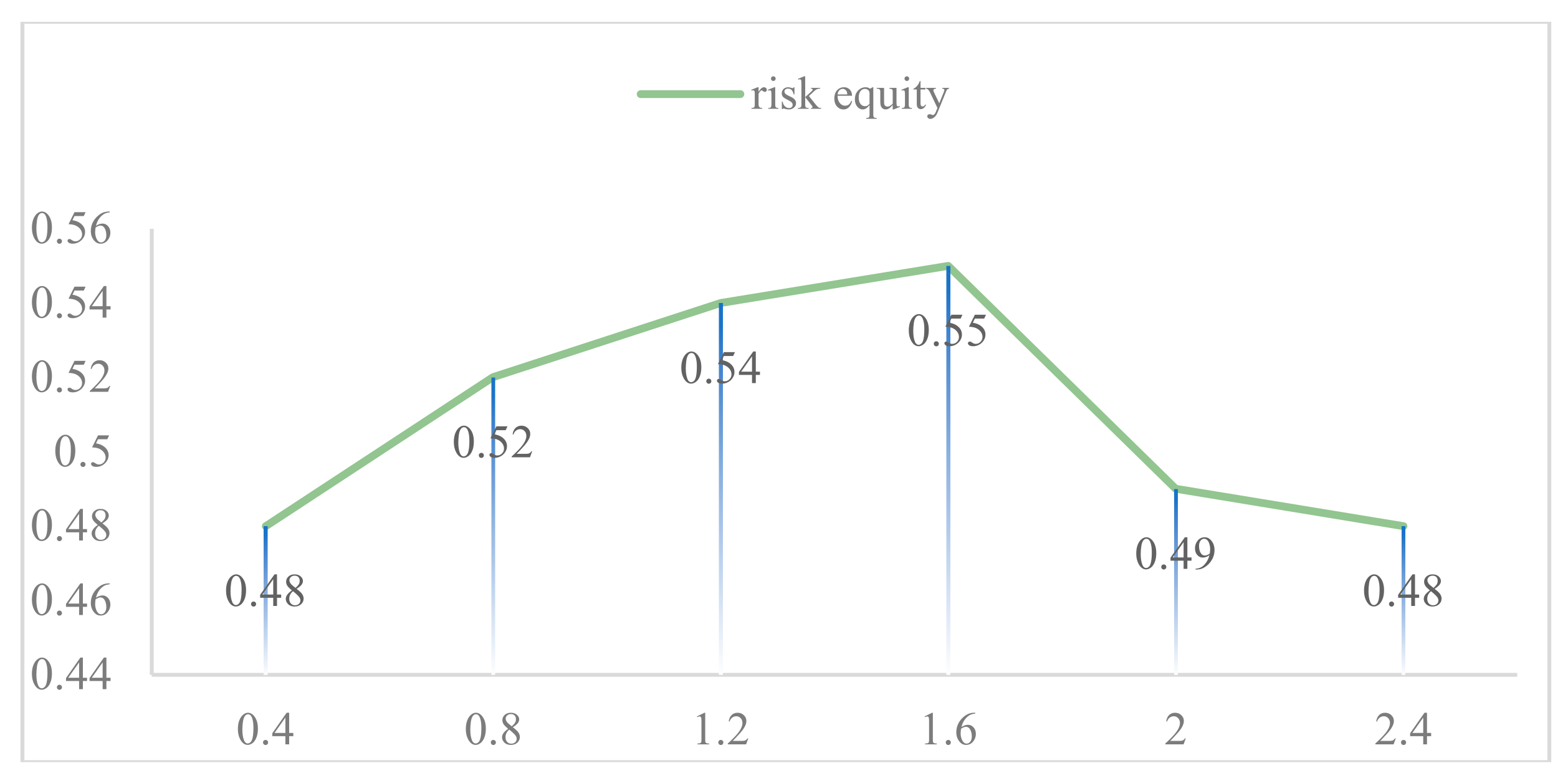
This finding has significant implications for government and enterprise management in the transportation of hazardous chemicals. Governments and enterprises should place great emphasis on the impact of wind speed and develop corresponding transportation strategies based on different wind speed conditions during actual transportation processes. For instance, when wind speeds are low, they should be more cautious in selecting transportation routes, trying to avoid densely populated areas to reduce the consequences of potential catastrophic population exposure accidents; while at higher wind speeds, they can appropriately relax route restrictions, but still need to closely monitor risk changes to ensure transportation safety. At the same time, this provides a theoretical basis for further optimizing the risk assessment models for hazardous chemical transportation. Future research can consider incorporating the dynamic changes of wind speed more accurately into the models to improve the accuracy and reliability of risk assessment.
5. Conclusions
Hazardous material transportation decision-making is typically a multi-objective process, as each stakeholder, including transporters, managers, customers, and residents, have a unique and sometimes conflicting objective that must be considered during planning. In this paper, risk compensation costs are incorporated into an objective function to minimize based on transportation risk and cost minimization to distribute hazard risk over a given road network equitably.
(1) Propose a time-varying risk equity and risk assessment model. This paper describes different affected areas according to different wind speed conditions, and considers different population density, wind speed, traffic flow and other factors under time variables to build a risk assessment function and a risk equity function under time-varying conditions. That can make full use of a variety of real-time and static data to assess the risk of hazardous chemical transportation more scientifically and reasonably.
(2) A time-varying multi-objective optimization model for hazardous materials transportation routes under time-varying conditions considering risk equity is established from the public viewpoint, taking into account the time, wind speed and risk differences in the network. The planning takes into account the government’s risk aversion considerations, the road operator’s cost viewpoint, and the public’s equity demands, and takes the Shanghai dangerous goods problem as an example.
In this study, the influence of node type on transportation risk was neglected in the time-varying risk assessment model of toxic gas transportation leakage from vehicles. In the future, the influence of node type on transportation risk can be further refined to more realistically reflect the risk of the complete transportation route.
Author Contributions
Liping Liu: Writing- original draft preparation, Data curation, Conceptualization. Tong Tian: writing—review and editing, Methodology, software. Rui Wang: Writing- review & editing, formal analysis, . Shuxia Li: Supervision, Project administration, Validation, Conceptualization.
Data Availability Statement
Data will be made available on request.
Acknowledgments
This work is funded by the National Natural Science Foundation of China (72442009, 72032001, 72074076, 71302043); Ministry of Education, Humanities and Social Sciences Research Planning Foundation (21YJA630057).
Conflicts of Interest
The authors declare that they have no known competing financial interests or personal relationships that could have appeared to influence the work reported in this paper.
References
- Holeczek, N. (2019). Hazardous materials truck transportation problems: a classification and state of the art literature review. Transportation Research, 69(APR.), 305-328.
- Keeney R, L. Equity and Public Risk[J]. Operations Research, 1980, 28(3): 527-534.
- Landucci G, Antonioni G, Tugnoli A, et al. HazMat transportation risk assessment: A revisitation in the perspective of the Viareggio LPG accident[J]. Journal of Loss Prevention in the Process Industries, 2017, 49: 36-46.
- Erkut E, Tjandra S A, Verter V. Hazardous materials transportation[J]. Handbooks in operations research and management science, 2007, 14: 539-621.
- Erkut E, Verter V. Modeling of transport risk for hazardous materials[J]. Operations research, 1998, 46(5): 625-642.
- Bula, G.A. Afsar, H.M., González, F.A., Prodhon, C., Velasco, N., 2019. Bi-objective vehicle routing problem for hazardous materials transportation. J. Clean. Prod. 206, 976-986.
- Jiang, P. , Men, J., Xu, H., Zheng, S., Kong, Y., Zhang, L., 2020. A variable neighborhood search-based hybrid multiobjective evolutionary algorithm for hazmat heterogeneous vehicle routing problem with time windows. IEEE Syst. J. 14, 4344–4355.
- Men, J. , Jiang, P., Xu, H., Zheng, S., Kong, Y., Hou, P., Wu, F., 2020a. Robust multi-objective vehicle routing problem with time windows for hazardous materials transportation. IET Intell. Transp. Syst. 14, 154-163.
- Jabbarzadeh A, Azad N, Verma M. An optimization approach to planning rail hazmat shipments in the presence of random disruptions[J]. Omega, 2020, 96: 102078.
- Ma T, Ma T, Wang Z,et al. Real-time risk assessment model for hazmat release accident involving tank truck[J]. Journal of Loss Prevention in the Process Industries, 2022, 77: 104759.
- Tan Y, Ma R, Sun Z, et al. Emission exposure optimum for a single-destination dynamic traffic network[J]. Transportation Research Part D: Transport and Environment, 2021, 94: 102817.
- Zhang P, Lan H. Effects of ventilation on leakage and diffusion law of gas pipeline in utility tunnel[J]. Tunnelling and Underground Space Technology, 2020, 105: 103557.
- Wang H Y, Zhang Q S. A Model for Obnoxious Effect of Waste Disposal Facilities Measurement Based on Improved Gaussian Plume Model[J]. Chinese Journal of Management Science,2012,20(02):102-106.
- Wang Y, Ren D, et al. Lou. PM2.5 concentration model of GNSS precipitable water vapor, wind speed and PM10 based on wavelet transform and regression analysis[J]. Systems Engineering-Theory & Practice,2020,40(03):761-770.
- Zandieh F, Ghannadpour S F. A comprehensive risk assessment view on interval type-2 fuzzy controller for a time-dependent HazMat routing problem[J]. European Journal of Operational Research, 2023, 305(2): 685-707.
- Ke G Y.Managing reliable emergency logistics for hazardous materials[J]. Computers & Operations Research, 2022, 138: 105557.
- ANDROUTSOPOULOS K N, ZOGRAFOS K G. A bi-objective time-dependent vehicle routing and scheduling problem for hazardous materials distribution[J]. EURO Journal on Transportation and Logistics, 2012, 1(1/2):157-183.
- Desai S, Lim G J. Solution time reduction techniques of a stochastic dynamic programming approach for hazardous material route selection problem[J]. Computers & Industrial Engineering, 2013, 65(4): 634-645.
- Chiou S, W. A resilience-based signal control for a time-dependent road network with hazmat transportation[J]. Reliability Engineering & System Safety, 2020, 193: 106570.
- Fontaine P, Crainic T G, Gendreau M, et al. Population-based risk equilibration for the multimode hazmat transport network design problem [J]. European Journal of Operational Research, 2020, 284(1): 188-200.
- Bhavsar N, Verma M. A subsidy policy to managing hazmat risk in railroad transportation network[J]. European Journal of Operational Research, 2022, 300(2): 633-646.
- Hosseini S D, Verma M. Equitable routing of rail hazardous materials shipments using CVaR methodology[J]. Computers & Operations Research, 2021, 129: 105222.
- Taslimi M, Batta R, Kwon C. A comprehensive modeling framework for hazmat network design, hazmat response team location, and equity of risk[J]. Computers & Operations Research, 2017, 79: 119-130.
- Ke G Y, Zhang H, Bookbinder J H. A dual toll policy for maintaining risk equity in hazardous materials transportation with fuzzy incident rate[J]. International journal of production economics, 2020, 227: 107650.
- Zhao J, Verter V. A bi-objective model for the used oil location-routing problem[J]. Computers & Operations Research, 2014, 62(oct.): 157-168.
- Zhang J, Hodgson J, Erkut E. Using GIS to assess the risks of hazardous materials transport in networks[J]. European Journal of Operational Research, 2000, 121(2): 316-329.
- Huang S, Chang Z, Wang Y, et al. Design and implementation of air pollution management system and an application case in Beijing[J]. IOP Conference Series: Earth and Environmental Science, 2021, 675(1): 012047 (7pp).
- Xuhai P, Juncheng J, Zhirong W. Numerical analysis of diffusion process of flammable and toxic gases discharging accident[J]. Progress in safety science and technology, 2000: 297-301.
- XIA D, QIAN X, HUANG J, et al. Diffusion simulation and hazard evaluation for liquid ammonia leakage[J]. China Safety Science Journal, 2014, 24(3): 22-27.
- Mavrotas, G. Effective implementation of the ε-constraint method in multi-objective mathematical programming problems[J]. Applied mathematics and computation, 2009, 213(2): 455-465.
- Mavrotas G, Florios K. An improved version of the augmented ε-constraint method (AUGMECON2) for finding the exact pareto set in multi-objective integer programming problems[J]. Applied Mathematics and Computation, 2013, 219(18): 9652-9669.
- DEB K, JAIN H. An evolutionary many-objective optimization algorithm using reference-point-based nondominated sorting approach, Part I: Solving problems with box constraints[J]. IEEE Transactions on Evolutionary Computation, 2014, 18(4): 577-601.
- Kuo R J, Edbert E, Zulvia F E, et al. Applying NSGA-II to vehicle routing problem with drones considering makespan and carbon emission[J]. Expert Systems with Applications, 2023, 221: 119777.
- Menares F, Montero E, Paredes-Belmar G, et al. A bi-objective time-dependent vehicle routing problem with delivery failure probabilities[J]. Computers & Industrial Engineering, 2023, 185: 109601.
- Gou M Y, Wang Y, Luo S Y, et al. Open-Closed Mixed Electric Vehicle Routing Optimization of Multi-center Distribution with Time Windows [J/OL]. Chinese Journal of Management Science, 2024, 1-17.
- Wang Y, Zhang J, Liu Y, et al. Optimization of Fresh Goods Multi-Center Vehicle Routing Problem Based on Resource Sharing and Temperature Control [J]. Chinese Journal of Management Science, 2022, 30(11): 272-285.
Figure 1.
Gaussian diffusion model coordinate system.
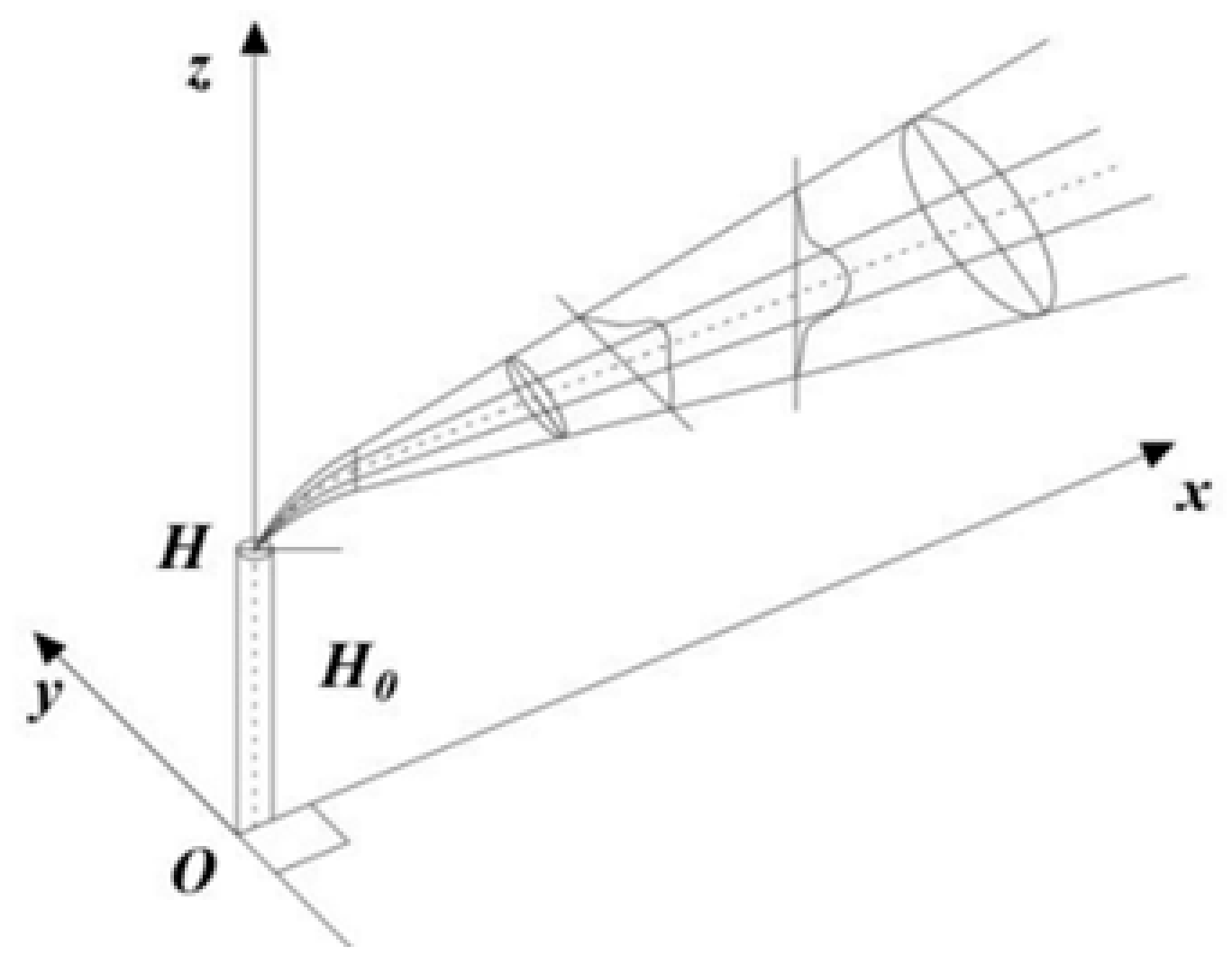
Figure 2.
Area of influence of gaseous hazards under windy conditions.
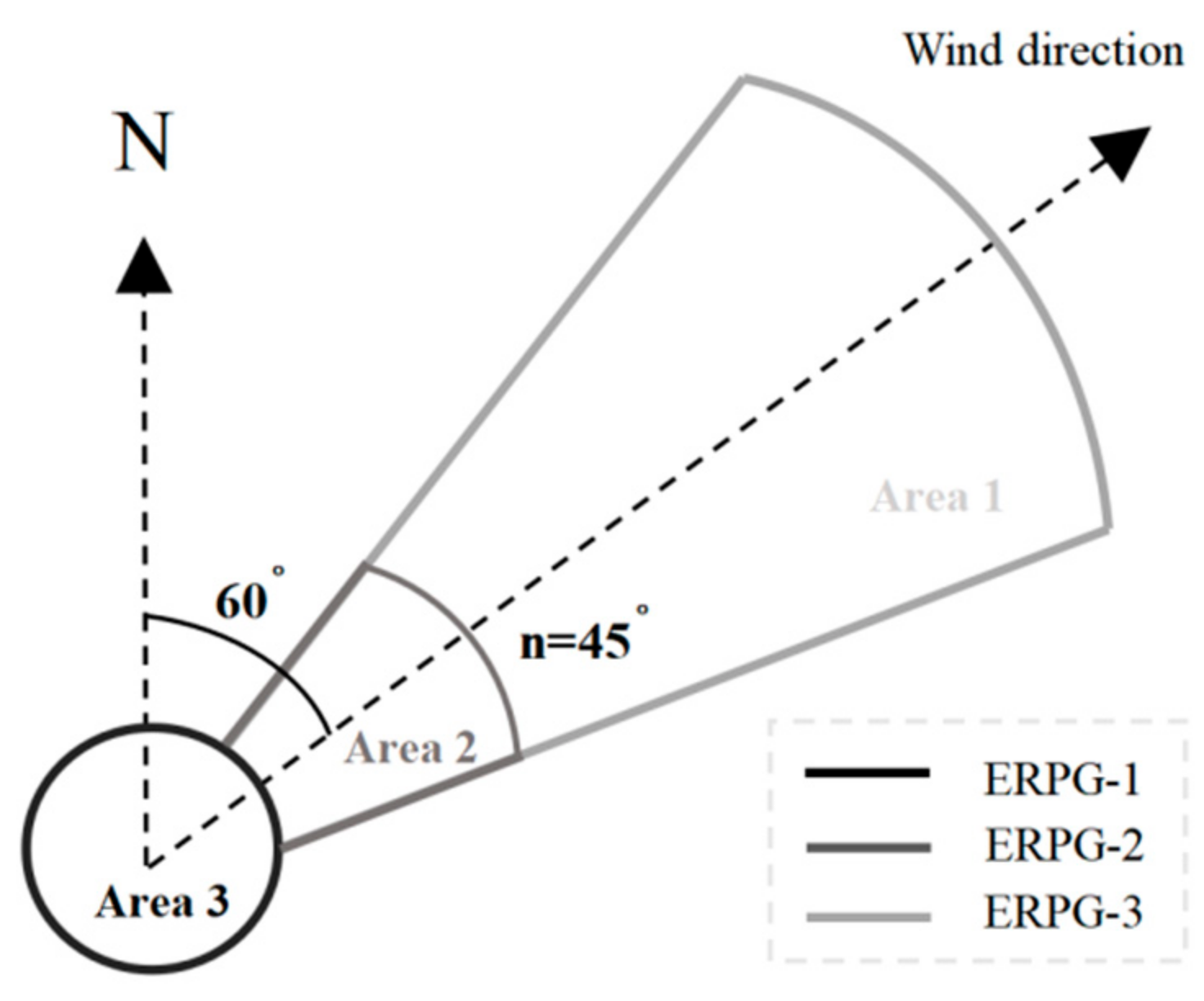
Figure 3.
Concentric circle simplified model of gaseous hazardous material impact area under light air and no wind conditions.
Figure 3.
Concentric circle simplified model of gaseous hazardous material impact area under light air and no wind conditions.
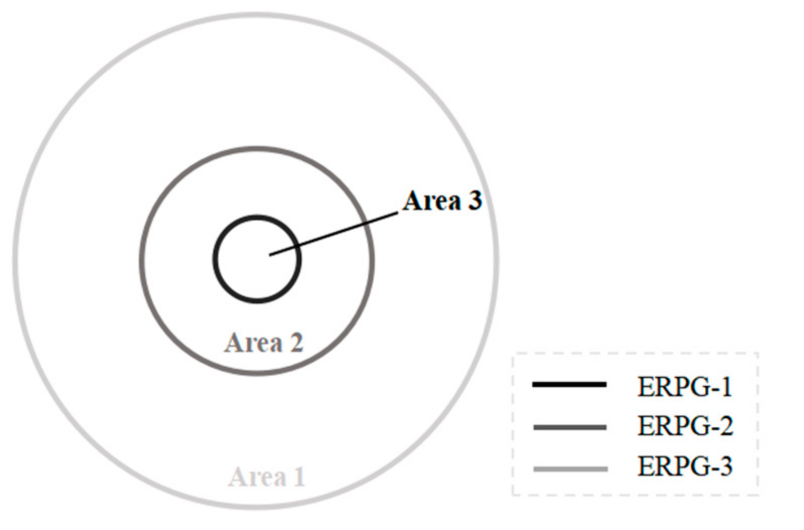
Figure 4.
The flowchart of Genetic Algorithm.
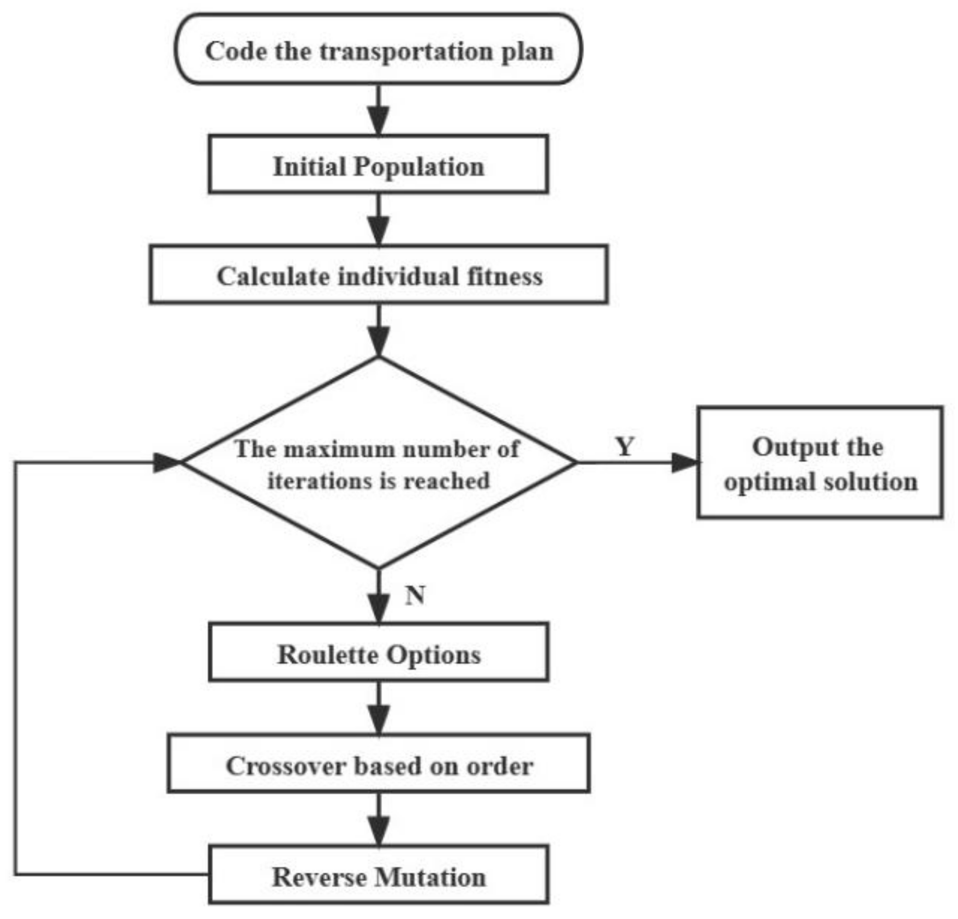
Figure 5.
Simplified diagram of the Shanghai transportation network.
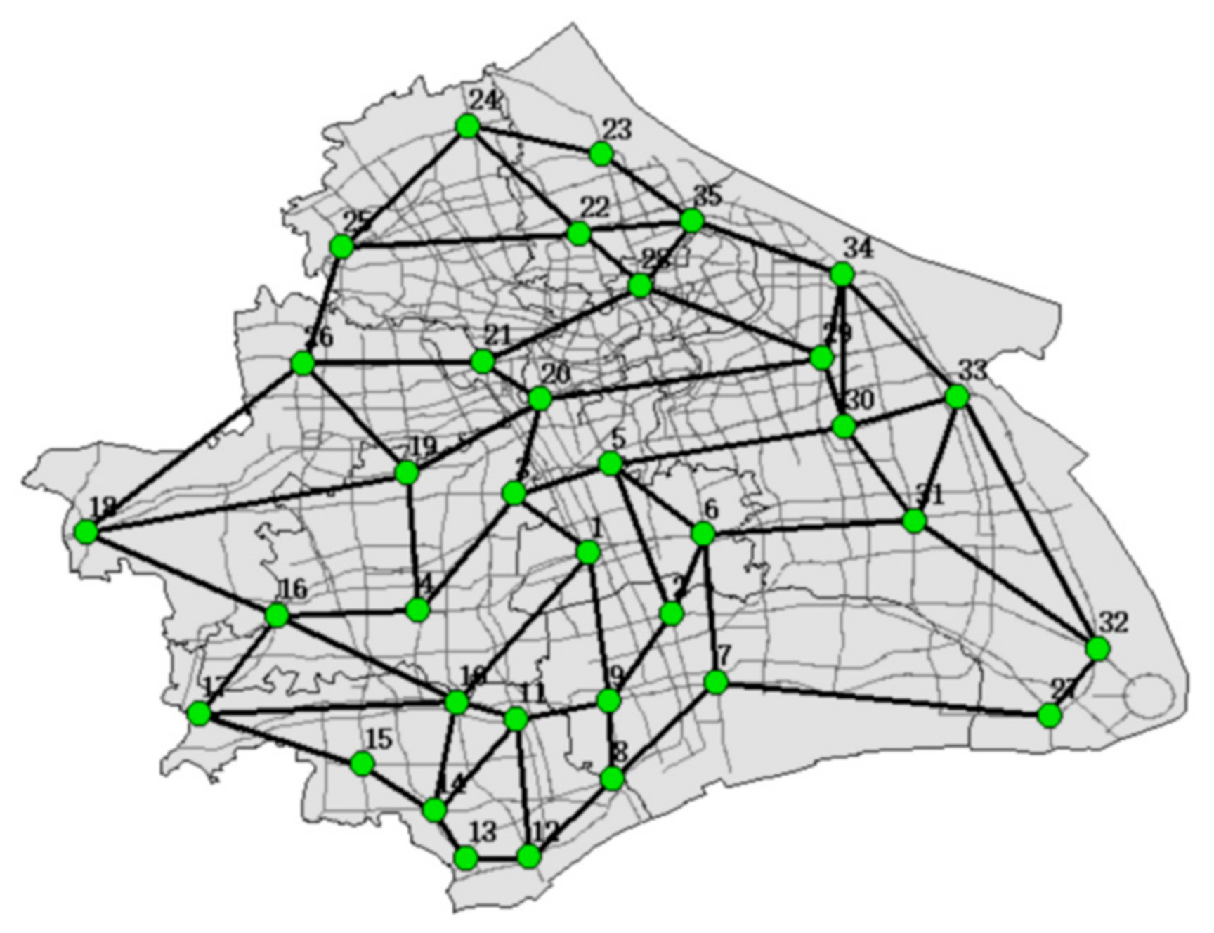
Figure 6.
Comparison of route with and without risk equity: (a) Optimal route without considering risk equity; (b) Optimal route with risk equity considered.
Figure 6.
Comparison of route with and without risk equity: (a) Optimal route without considering risk equity; (b) Optimal route with risk equity considered.
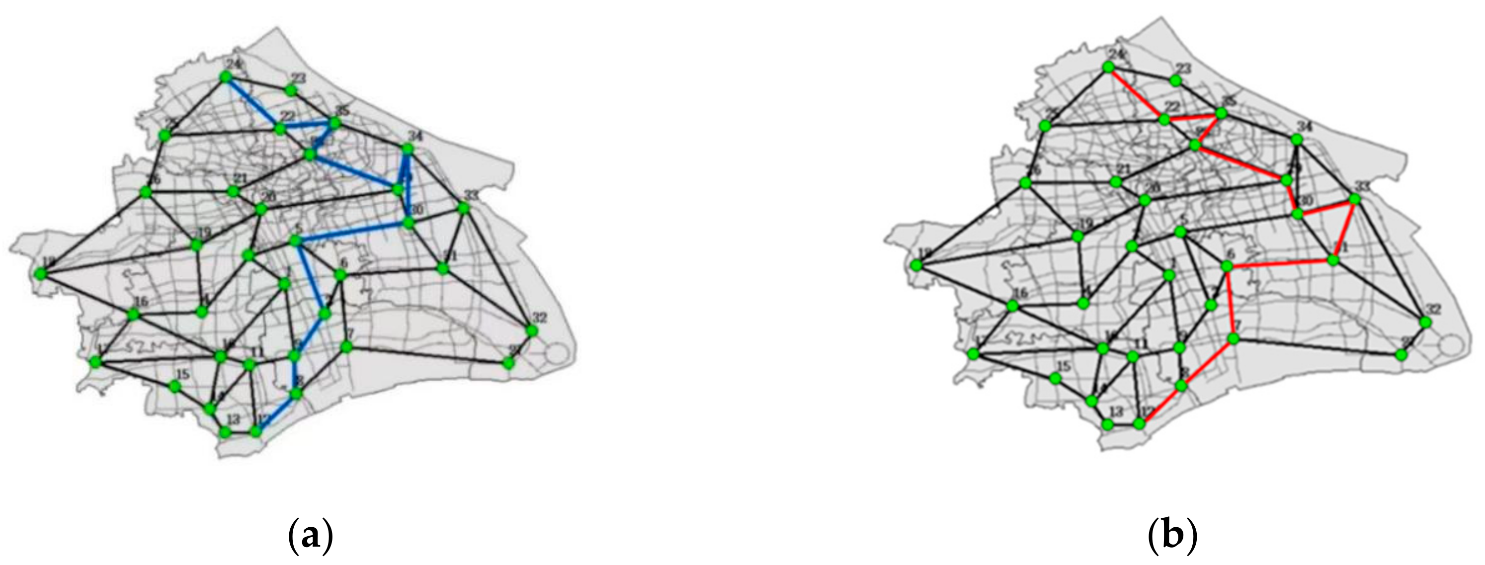
Figure 7.
Optimal route with risk equity considered. (a) t[3,5],[9,11],[12,13],[14,17],[18,19],[21,24]; (b) t[1,2],[6,7]; (c) t[0,1],[2,3],[5,6],[7,9],[11,12],[13,14],[19,21]; (d) t [18,19]; (e) t [17,18].
Figure 7.
Optimal route with risk equity considered. (a) t[3,5],[9,11],[12,13],[14,17],[18,19],[21,24]; (b) t[1,2],[6,7]; (c) t[0,1],[2,3],[5,6],[7,9],[11,12],[13,14],[19,21]; (d) t [18,19]; (e) t [17,18].

Table 5.
24-hour Hazardous Chemical Transportation Route.
| The 24-hour period |
Aggregate risk | Gini coefficient |
trails |
|---|---|---|---|
| 0:00-1:00 | 1598.69 | 0.286 | 24-22-35-28-29-34-35-5-2-9-11-12 |
| 1:00-2:00 | 1281.81 | 0.217 | 24-22-35-28-29-34-35-5-6-2-9-11-12 |
| 2:00-3:00 | 1844.64 | 0.286 | 24-22-35-28-29-34-35-5-2-9-11-12 |
| 3:00-4:00 | 2136.35 | 0. 327 | 24-22-35-28-29-34-30-5-2-9-8-12 |
| 4:00-5:00 | 2319.47 | 0. 327 | 24-22-35-28-29-34-30-5-2-9-8-12 |
| 5:00-6:00 | 2766.97 | 0.286 | 24-22-35-28-29-34-35-5-2-9-11-12 |
| 6:00-7:00 | 3465.71 | 0.217 | 24-22-35-28-29-34-35-5-6-2-9-11-12 |
| 7:00-8:00 | 3074.41 | 0.286 | 24-22-35-28-29-34-35-5-2-9-11-12 |
| 8:00-9:00 | 6087.32 | 0.286 | 24-22-35-28-29-34-35-5-2-9-11-12 |
| 9:00-10:00 | 7935.02 | 0. 327 | 24-22-35-28-29-34-30-5-2-9-8-12 |
| 10:00-11:00 | 7629.82 | 0. 327 | 24-22-35-28-29-34-30-5-2-9-8-12 |
| 11:00-12:00 | 7378.57 | 0.286 | 24-22-35-28-29-34-35-5-2-9-11-12 |
| 12:00-13:00 | 8179.17 | 0. 327 | 24-22-35-28-29-34-30-5-2-9-8-12 |
| 13:00-14:00 | 6456.25 | 0.286 | 24-22-35-28-29-34-35-5-2-9-11-12 |
| 14:00-15:00 | 5615.55 | 0. 327 | 24-22-35-28-29-34-30-5-2-9-8-12 |
| 15:00-16:00 | 7019.44 | 0. 327 | 24-22-35-28-29-34-30-5-2-9-8-12 |
| 16:00-17:00 | 7935.02 | 0. 327 | 24-22-35-28-29-34-30-5-2-9-8-12 |
| 17:00-18:00 | 10048.91 | 0.431 | 24-22-35-28-29-30-34-33-31-6-2-9-8-12 |
| 18:00-19:00 | 7629.82 | 0. 327 | 24-22-35-28-29-34-30-5-2-9-8-12 |
| 19:00-20:00 | 7378.57 | 0.286 | 24-22-35-28-29-34-35-5-2-9-11-12 |
| 20:00-21:00 | 6456.25 | 0.286 | 24-22-35-28-29-34-35-5-2-9-11-12 |
| 21:00-22:00 | 5371.40 | 0. 327 | 24-22-35-28-29-34-30-5-2-9-8-12 |
| 22:00-23:00 | 3996.73 | 0. 327 | 24-22-35-28-29-34-30-5-2-9-8-12 |
| 23:00-24:00 | 3357.12 | 0. 327 | 24-22-35-28-29-34-30-5-2-9-8-12 |
Table 6.
Consequences of road transportation leakage accident at time t.
| Link | Area of different hazardous areas(k㎡) | Accident Consequences |
||
|---|---|---|---|---|
| ERPG_3 | ERPG_2 | ERPG_1 | ||
| 1-2 | 4.93 | 8.86 | 9.58 | 2766.67 |
| 1-3 | 6.74 | 12.11 | 13.1 | 4075.44 |
| 2-3 | 1.82 | 3.27 | 3.54 | 1413.89 |
| 2-23 | 10.16 | 18.27 | 19.76 | 5704.78 |
| 3-4 | 2.43 | 4.37 | 4.72 | 6488.17 |
| 24-22 | 6.03 | 10.83 | 11.72 | 16447.6 |
| 25-8 | 5.46 | 9.81 | 10.62 | 21013.59 |
| 13-25 | 3.79 | 6.82 | 7.37 | 12955.8 |
| 26-35 | 3.31 | 5.95 | 6.44 | 12637.88 |
| 26-42 | 4.55 | 8.18 | 8.85 | 17373.61 |
Disclaimer/Publisher’s Note: The statements, opinions and data contained in all publications are solely those of the individual author(s) and contributor(s) and not of MDPI and/or the editor(s). MDPI and/or the editor(s) disclaim responsibility for any injury to people or property resulting from any ideas, methods, instructions or products referred to in the content. |
© 2025 by the authors. Licensee MDPI, Basel, Switzerland. This article is an open access article distributed under the terms and conditions of the Creative Commons Attribution (CC BY) license (http://creativecommons.org/licenses/by/4.0/).
Copyright: This open access article is published under a Creative Commons CC BY 4.0 license, which permit the free download, distribution, and reuse, provided that the author and preprint are cited in any reuse.


