1. Introduction
In recent years, machine learning methods have achieved remarkable success across diverse domains. Among various machine learning approaches, Tree-based Ensemble Models have garnered significant attention from both academia and industry due to their distinctive advantages. These models not only effectively handle non-linear relationships but also perform automatic feature selection while maintaining robust performance in the presence of outliers. More significantly, compared to black-box models such as neural networks, tree models offer superior interpretability, providing them with a distinct advantage in applications requiring decision explanations.
Tree-based models have established themselves as fundamental tools for solving complex problems in finance. In their study of U.S. financial institution bankruptcy prediction, Petropoulos et al. (2020) demonstrated that random forest models exhibit superior performance in both out-of-sample and out-of-time predictions, while effectively identifying key predictive factors within the CAMELS evaluation framework. Through their comprehensive benchmark study of credit scoring algorithms, Lessmann et al. (2015) systematically evaluated contemporary classification algorithms including tree models, providing crucial insights into technical advancements in credit scoring practice. Research by Carmona et al. (2019) revealed that tree models perform exceptionally well in predicting U.S. bank failures, particularly during extreme market conditions such as financial crises.
Tree models have also found extensive applications in asset pricing, primarily addressing two crucial challenges: improving return prediction accuracy and identifying key pricing factors. Nti et al. (2019) applied random forest methodology to stock market prediction, effectively identifying key macroeconomic variables through feature selection, demonstrating superior accuracy compared to traditional methods. Gu et al. (2020) showed that tree models excel in both return prediction and feature contribution quantification. Lin et al. (2022), in their comprehensive survey, revealed tree models' significant advantages in handling non-linear relationships and high-dimensional data. For feature importance identification, Gu et al. (2020) and Leippold et al. (2021) assessed feature importance through variable removal impact, while Ma et al. (2023) employed SHAP methodology. However, these approaches generally overlook the dynamic characteristics of time series data.
Despite their achievements in asset pricing and feature identification, traditional tree models exhibit several limitations in processing large-scale financial data. These models often face challenges in computational efficiency and memory utilization when handling high-dimensional datasets with hundreds of thousands of records (Ferrouhi and Bouabdallaoui, 2024; Siswara et al., 2024). LightGBM (Ke et al., 2017) addresses these challenges through its histogram-based algorithm and leaf-wise growth strategy, enhancing both computational efficiency and memory utilization for large-scale asset pricing research.
Building on these advantages of LightGBM, this study aims to apply it to asset return prediction and feature importance identification. The methodology not only promises to enhance predictive accuracy but also provides new empirical insights into asset pricing theory. Through comparative analysis against traditional econometric methods and other machine learning algorithms, this paper comprehensively evaluates its applicability in asset pricing. Additionally, the feature importance analysis offered by LightGBM helps uncover key factors influencing asset returns, which is crucial for constructing more robust investment strategies and deepening our understanding of market dynamics.The remainder of this paper is organized as follows:
Section 2 presents the research design.
Section 3 describes the dataset used in this study.
Section 4 presents the empirical results. Section 5 concludes the paper.
2. Data and Methodology
This study obtains daily stock return data for all A-shares listed on the Shanghai and Shenzhen Stock Exchanges from the Wind database and converts it to monthly frequency. After applying exclusion criteria—removing financial industry stocks, those with less than 12 months of listing history or fewer than 15 monthly trading days, ST-designated stocks, those with negative net assets—the final sample includes 4885 A-share stocks from the Main Board, ChiNext Board, and STAR Market traded from January 2000 to December 2023. Quarterly financial statement data is obtained from CSMAR, which also provides the one-year Chinese government bond yield as the risk-free rate proxy. Based on historical literature, I construct 50 stock characteristics, detailed in
Table A1 of the
Appendix A.
The analysis employs a generalized prediction error model to describe the relationship between stock excess returns and stock characteristics. The basic form of the model can be expressed as:
where
represents the excess return of stock
at time
,
is the conditional expectation based on information at time
, and
is the prediction error term. Furthermore, the conditional expectation of stock excess returns is assumed to be a function of stock characteristics:
where
is a matrix containing stock characteristics of stock
from time
to
.
represents the historical data window length,
is the number of predictive features (50 in this paper), θ represents the model hyperparameters, and
denotes the LightGBM function.
This study employs the LightGBM model to characterize the relationship between stock returns and firm characteristics. LightGBM is a gradient boosting framework based on decision trees that differs from traditional Gradient Boosting Decision Tree (GBDT) algorithms in its growth strategy. While GBDT uses a level-wise growth strategy, LightGBM implements a leaf-wise growth strategy. Under this strategy, the model iteratively selects the leaf node with maximum loss reduction for splitting, which can achieve lower loss compared to level-wise algorithms given the same number of splits. In LightGBM, the function
is modeled as a weighted sum of T decision trees:
where
represents the
-th decision tree and
is its corresponding weight coefficient. Each decision tree is trained to minimize the following objective function:
where
denotes the loss function,
is the regularization term that penalizes model complexity, and
is the regularization coefficient. In contrast to traditional GBDT algorithms that employ level-wise growth strategy, LightGBM adopts a leaf-wise growth strategy, where the model iteratively selects the leaf node with maximum loss reduction for splitting, achieving lower loss compared to level-wise algorithms with the same number of splits.
For feature importance identification, LightGBM employs a split-gain-based approach to evaluate feature importance by calculating the total gain generated by each feature during the decision tree splitting process. The larger the gain produced by a feature during splitting, the more significant its contribution to improving the model's predictive capability. For feature k, its importance score can be expressed as:
where
and
represent the loss function values before and after splitting using the feature, respectively. Theoretically, a larger split gain indicates that the split is more effective in reducing the model's prediction error, thereby indicating the feature's greater importance for prediction.
Finally, this study adopts the same sample splitting scheme as Leippold et al. (2021). The dataset is divided into three non-overlapping time periods: training set (2000-2010), validation set (2011-2013), and test set (2014-2023). When the model begins a new round of training, the training set incorporates the next year's data while retaining its original data; the validation set and the one-year test set move forward accordingly to include the next 12 months of data. Model training is conducted annually in January rather than monthly.
3. Results
This section presents the empirical results. The analysis begins with a comparison of LightGBM and traditional Ordinary Least Squares (OLS) regression in predicting excess returns in Chinese A-shares. This is followed by an examination of feature importance and its economic implications.
Table 1 presents a comparison of out-of-sample predictive performance between LightGBM and OLS regression, measured by the R-squared (R²) statistic. The empirical results indicate that LightGBM achieves a monthly out-of-sample R² of 2.13%, representing a substantial improvement over the traditional OLS approach which yields an R² of 0.95%. This marked enhancement in predictive accuracy suggests that LightGBM's non-linear framework better captures the inherent complexities in stock return patterns that elude linear regression methods.
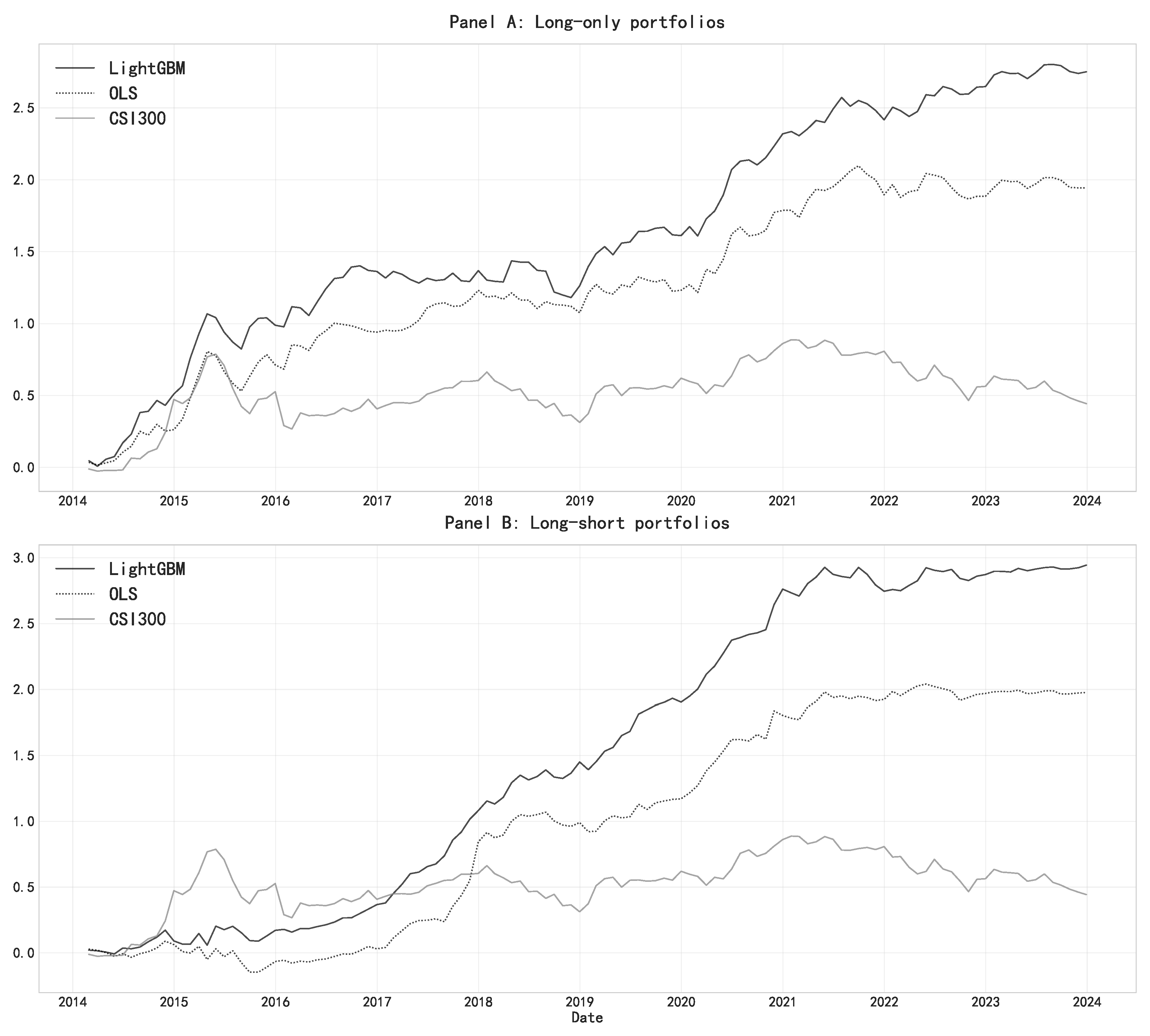
Table 2 explores the economic significance of predictive performance through portfolio analysis. For the long-only strategy, LightGBM achieves a higher average monthly return of 2.54% compared to 1.83% for OLS, with an improved Sharpe ratio of 1.34 versus 1.01. The long-short strategy demonstrates even stronger performance under LightGBM, yielding a monthly return of 2.63% and a Sharpe ratio of 1.77, substantially outperforming the OLS approach which generates a return of 1.82% and a Sharpe ratio of 1.11. Notably, LightGBM also exhibits better downside protection, with less severe maximum drawdowns in both strategies (-22.55% versus -24.13% for long-only, and -16.60% versus -21.09% for long-short).
Figure 1 depicts the cumulative performance of different investment strategies relative to the CSI 300 index, which is a capitalization-weighted stock market index designed to track the performance of 300 most representative stocks listed on the Shanghai and Shenzhen Stock Exchanges. Panel A demonstrates that the LightGBM-based long-only strategy consistently outperforms both the OLS approach and the CSI 300 benchmark, with the outperformance becoming particularly pronounced after 2020. The superior performance of LightGBM is even more evident in Panel B's long-short strategy, where it achieves a cumulative log return of approximately 3.0 by 2024, substantially exceeding both the OLS strategy and the market benchmark.
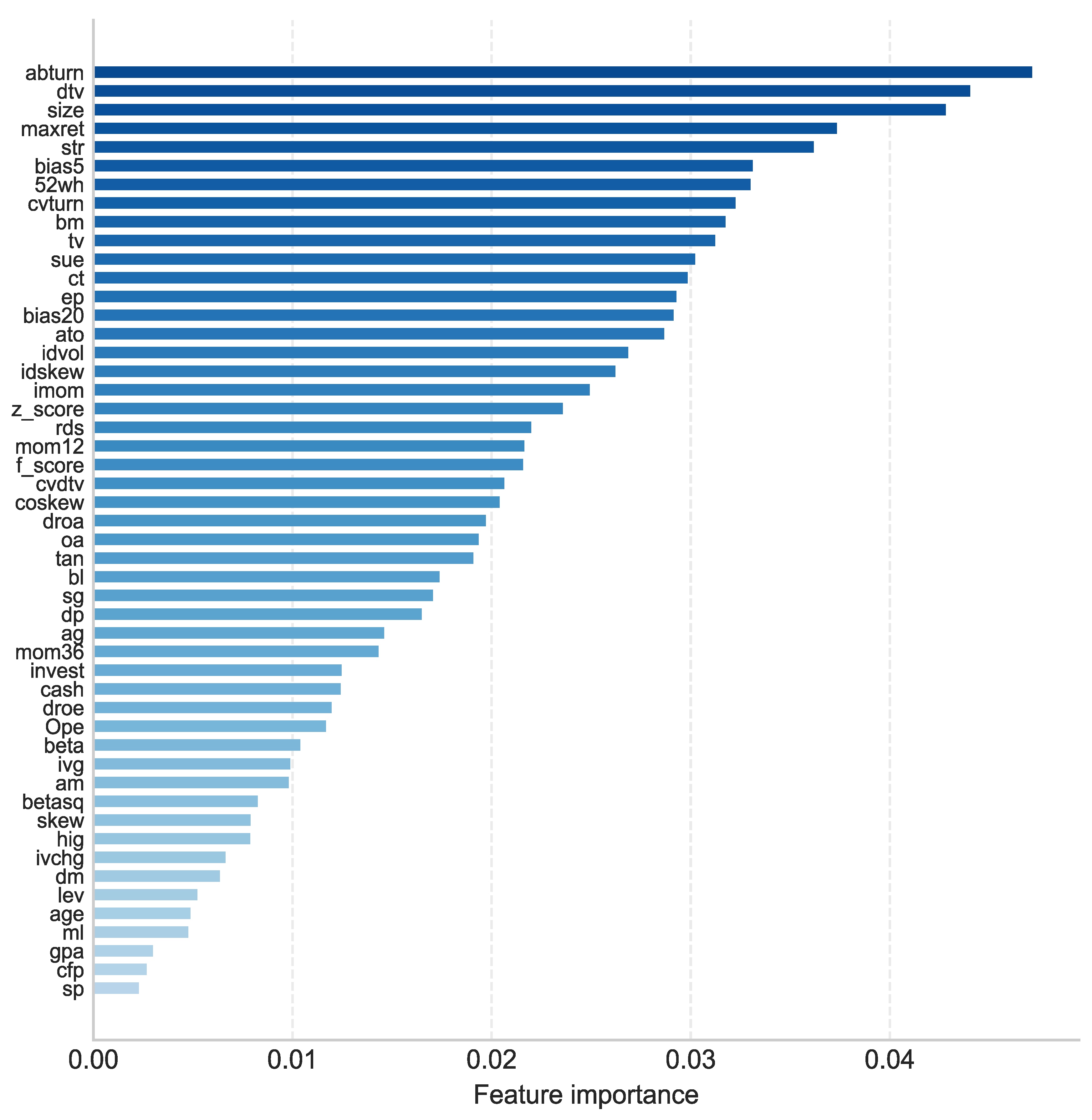
Beyond predictive performance, understanding the relative importance of different features in explaining stock returns is another crucial aspect of asset pricing research. Based on the split-gain calculation specified in Equation (5),
Figure 2 presents the feature importance scores derived from the LightGBM model. Consistent with Leippold et al. (2021), the results suggest that both liquidity and volatility-related characteristics are the most influential predictors in the Chinese A-share market. Specifically, liquidity measures, including abnormal turnover (abturn), trading volume (dtv), market capitalization (size), and trading volume variation (cvturn), rank among the top predictors. Volatility indicators such as maximum daily return (maxret) and historical price deviation (bias5) also demonstrate significant predictive power.
4. Conclusions
This study demonstrates the effectiveness of LightGBM in predicting stock returns and identifying key pricing factors in the Chinese A-share market. The empirical results reveal two main findings. First, LightGBM significantly outperforms traditional OLS regression in return prediction, achieving a monthly out-of-sample R² of 2.13% compared to 0.95% for OLS. This superior predictive power translates into substantial economic gains, with the LightGBM-based long-short strategy generating a monthly return of 2.63% and a Sharpe ratio of 1.77, while maintaining better downside protection.
Second, the feature importance analysis provides new insights into the return-generating process in China's stock market. Consistent with Leippold et al. (2021), liquidity and volatility-related characteristics emerge as the dominant predictors, with measures such as abnormal turnover, trading volume, and price volatility demonstrating the strongest predictive power.
These findings have important implications for both academic research and investment practice. From an academic perspective, they highlight the value of machine learning approaches in capturing complex, non-linear relationships in asset pricing. For practitioners, the results suggest that incorporating advanced machine learning techniques and focusing on market microstructure factors could enhance investment strategies in the Chinese stock market.
Appendix A
Table A1.
Details on stock characteristics.
Table A1.
Details on stock characteristics.
| No |
Acronym |
Stock Characteristics |
Author(s) |
Year, Journal |
| 1 |
abturn |
Abnormal turnover |
Liu et al. |
2016, JFE |
| 2 |
ag |
Asset growth |
Cooper et al. |
2008, JF |
| 3 |
age |
Firm age |
Jiang et al. |
2005, RAS |
| 4 |
am |
Asset to market equity |
Bhandari |
1988, JF |
| 5 |
ato |
Asset turnover |
Soliman |
2008, TAR |
| 6 |
beta |
Beta |
Fama & MacBeth |
1973, JPE |
| 7 |
betasq |
Beta squared |
Fama & MacBeth |
1973, JPE |
| 8 |
bias5 |
The 5-day bias |
Zhang & Wu |
2009, ESA |
| 9 |
bias20 |
The 20-day bias |
Zhang & Wu |
2009, ESA |
| 10 |
bl |
Book leverage |
Fama & French |
1992, JF |
| 11 |
bm |
Book to market |
Rosenberg et al. |
1985, JPM |
| 12 |
cash |
Cash holdings |
Palazzo |
2012, JFE |
| 13 |
cfp |
Cash flow to price |
Desai et al. |
2004, TAR |
| 14 |
coskew |
Skewness coefficient |
Harvey & Siddique |
1999, JFQA |
| 15 |
ct |
Capital turnover |
Hou et al. |
2020, RFS |
| 16 |
cvturn |
Coefficient of Variation of Share Turnover |
Chordia et al. |
2001, JFE |
| 17 |
cvdtv |
Coefficient of Variation of Trading Volume |
Chordia et al. |
2001, JFE |
| 18 |
dm |
Debt to market equity |
Hou et al. |
2020, RFS |
| 19 |
dp |
Dividend to price |
Litzenberger et al. |
1982, JF |
| 20 |
dtv |
Trading volume |
Brennan et al. |
1998, JFE |
| 21 |
droa |
Change in return on asset |
Hou et al. |
2020, RFS |
| 22 |
droe |
Change in return on equity |
Hou et al. |
2020, RFS |
| 23 |
ep |
Earnings to price |
Basu |
1977, JF |
| 24 |
f_score |
F score |
Piotroski |
2000, JAR |
| 25 |
gpa |
Gross profit to asset |
Novy-Marx |
2013, JFE |
| 26 |
hig |
Employee growth rate |
Bazdresch et al. |
2014, JPE |
| 27 |
idvol |
Idiosyncratic volatility |
Ali et al. |
2003, JFE |
| 28 |
idskew |
Idiosyncratic skewness |
Boyer et al. |
2010, RFS |
| 29 |
imom |
Idiosyncratic momentum |
Blitz et al. |
2011, JEF |
| 30 |
invest |
Capital expenditures and inventory |
Chen & Zhang |
2010, JF |
| 31 |
ivchg |
Inventory changes |
Hou et al. |
2020, RFS |
| 32 |
ivg |
Inventory growth |
Hou et al. |
2020, RFS |
| 33 |
lev |
Leverage |
Bhandari |
1988, JF |
| 34 |
maxret |
Maximum daily return |
Bali et al. |
2011, JFE |
| 35 |
mom12 |
12-month momentum |
Jegadeesh |
1990, JF |
| 36 |
mom36 |
36-month momentum |
Jegadeesh &Titman |
1993, JF |
| 37 |
ml |
Market leverage |
Fama & French |
1992, JF |
| 38 |
oa |
Operating accruals |
Hribar & Collins |
2002, JAR |
| 39 |
Ope |
Operating profits to book equity |
Fama & French |
2015, JFE |
| 40 |
rds |
R&D to sales |
Guo et al. |
2006, JBFA |
| 41 |
sp |
Sales to price |
Barbee et al. |
1996, FAJ |
| 42 |
skew |
Skew |
Amaya |
2015, JFE |
| 43 |
size |
Size |
Banz |
1981, JFE |
| 44 |
sue |
Standardized unexpected earnings |
Foster et al. |
1984, TAR |
| 45 |
str |
Short term reversal |
Jegadeesh |
1990, JF |
| 46 |
sg |
Sales growth |
Lakonishok |
1994, JF |
| 47 |
tv |
Total volatility |
Ang et al. |
2010, JF |
| 48 |
tan |
Debt capacity/firm tangibility |
Almeida et al. |
2007, RFS |
| 49 |
52wh |
The highest return in 52-week |
George et al. |
2004, JF |
| 50 |
z_score |
Z score |
Altman |
1968, JF |
References
- Carmona, P.; Climent, F.; Momparler, A. Predicting failure in the US banking sector: An extreme gradient boosting approach. International Review of Economics & Finance 2019, 61, 304–323. [Google Scholar] [CrossRef]
- Chen, X.; Mao, Z.; Wu, C. Multi-class Financial Distress Prediction Based on Feature Selection and Deep Forest Algorithm. Computational Economics 2024, 1–40. [Google Scholar] [CrossRef]
- Deng, S.; Zhu, Y.; Huang, X.; Duan, S.; Fu, Z. High-frequency direction forecasting of the futures market using a machine-learning-based method. Future Internet 2022, 14, 180. [Google Scholar] [CrossRef]
- Ferrouhi, E.M.; Bouabdallaoui, I. A comparative study of ensemble learning algorithms for high-frequency trading. Scientific African 2024, 24, e02161. [Google Scholar] [CrossRef]
- Gu, S.; Kelly, B.; Xiu, D. Empirical asset pricing via machine learning. The Review of Financial Studies 2020, 33, 2223–2273. [Google Scholar] [CrossRef]
- Ke, G.; Meng, Q.; Finley, T.; Wang, T.; Chen, W.; Ma, W.; ...; Liu, T.Y. Lightgbm: A highly efficient gradient boosting decision tree. Advances in neural information processing systems 2017, 30. [Google Scholar]
- Leippold, M.; Wang, Q.; Zhou, W. Machine learning in the Chinese stock market. Journal of Financial Economics 2021, 145, 64–82. [Google Scholar] [CrossRef]
- Lessmann, S.; Baesens, B.; Seow, H.V.; Thomas, L.C. Benchmarking state-of-the-art classification algorithms for credit scoring: An update of research. European Journal of Operational Research 2015, 247, 124–136. [Google Scholar] [CrossRef]
- Lin, W.; Hu, Y.; Tsai, C. Machine learning in financial crisis prediction: A survey. IEEE Transactions on Systems, Man, and Cybernetics 2022, 42, 421–436. [Google Scholar] [CrossRef]
- Lundberg, S. A unified approach to interpreting model predictions. arXiv 2017, arXiv:1705.07874. [Google Scholar]
- Ma, T.; Wang, W.; Chen, Y. Attention is all you need: An interpretable transformer-based asset allocation approach. International Review of Financial Analysis 2023, 90, 102876. [Google Scholar] [CrossRef]
- Nti, K.O.; Adekoya, A.; Weyori, B. Random forest based feature selection of macroeconomic variables for stock market prediction. American Journal of Applied Sciences 2019, 16, 200–212. [Google Scholar] [CrossRef]
- Petropoulos, A.; Siakoulis, V.; Stavroulakis, E.; Vlachogiannakis, N.E. Predicting bank insolvencies using machine learning techniques. International Journal of Forecasting 2020, 36, 1092–1113. [Google Scholar] [CrossRef]
- Siswara, D.; Soleh, A.M.; Wigena, A.H. Classification Modeling with RNN-Based, Random Forest, and XGBoost for Imbalanced Data: A Case of Early Crash Detection in ASEAN-5 Stock Markets. arXiv 2024, arXiv:2406.07888. [Google Scholar]
|
Disclaimer/Publisher’s Note: The statements, opinions and data contained in all publications are solely those of the individual author(s) and contributor(s) and not of MDPI and/or the editor(s). MDPI and/or the editor(s) disclaim responsibility for any injury to people or property resulting from any ideas, methods, instructions or products referred to in the content. |
© 2025 by the authors. Licensee MDPI, Basel, Switzerland. This article is an open access article distributed under the terms and conditions of the Creative Commons Attribution (CC BY) license (http://creativecommons.org/licenses/by/4.0/).