
Submitted:
31 December 2024
Posted:
03 January 2025
You are already at the latest version
Abstract
Traditionally, classifying species has required taxonomic experts to carefully examine unique physical characteristics, a time-intensive and complex process. Machine learning offers a promising alternative by utilizing computational power to detect subtle distinctions more quickly and accurately. This technology can classify both known (described) and unknown (undescribed) species, assigning known samples to specific species and grouping unknown ones at the genus level—an improvement over the common practice of labeling unknown species as outliers. In this paper, we propose a novel ensemble approach that integrates neural networks with support vector machines (SVM). Each animal is represented by an image and its DNA barcode. Our research investigates the transformation of one-dimensional vector data into two-dimensional three-channels matrices using discrete wavelet transform (DWT), enabling the application of convolutional neural networks (CNNs) that have been pre-trained on large image datasets. Our method significantly outperforms existing approaches, as demonstrated on several datasets containing animal images and DNA barcodes. By enabling the classification of both described and undescribed species, this research represents a major step forward in global biodiversity monitoring. The MATLAB/PyTorch source code for our ensemble method, along with the datasets used in this study, will be publicly available at: https://github.com/LorisNanni/Advancing-Taxonomy-with-Machine-Learning-A-Hybrid-Ensemble-for-Species-and-Genus-Classification
Keywords:
ensemble
; convolutional neural networks
; support vector machine
; discrete wavelet
; DNA barcode
1. Introduction
Exploring biodiversity involves a complex and demanding process. It begins with extensive fieldwork, where entomologists venture into diverse and often remote habitats to gather specimens. These are subjected to rigorous identification procedures, including morphological assessments, genetic analyses, and taxonomic evaluations. This meticulous work is necessary for deepening our understanding of animal diversity, their ecological roles, evolutionary links, and interactions with human endeavors. For instance, it’s important to highlight that insects play a critical role in ecosystems, such as pollination, decomposition, and serving as a food source for other organisms. This underscores the urgency of cataloging and preserving their diversity.
In this paper, we mainly focus on insect datasets. Although an estimated 5.5 million insect species exist, only around 20% have been documented [1]. The challenge is intensified by the extinction of numerous species before they can be formally described [2].
In biology, taxonomy refers to the branch of science concerned with the conception, naming, and classification of groups of organisms. Modern classification divides any organism based on the Domain (Archaea, Bacteria and Eucarya) and then on Kingdom, Phylum, Class, Order, Family, Genus and Species. An example can be seen in Figure 1. Traditionally, taxonomists rely on morphological features to classify insects by their physical characteristics [3]. However, these keys are less effective for undescribed species with indistinct or missing diagnostic features. To address this limitation, DNA barcoding [4] serves as a complementary method, using genetic variation to identify species when phenotypic traits are insufficient [5].
Identifying insect species remains a major challenge. Although the DNA Barcode Database (BOLD) [6] holds a large amount of genetic data, most of it is not related to known species. This mismatch reveals the slow progress in identification, made worse by a shortage of taxonomists and a decline in traditional taxonomy practices, as explained in [7]. To address this, there is an urgent need for faster and more efficient methods to uncover and classify species.
Machine learning (ML) techniques present innovative solutions by analyzing complex data patterns to classify species and detect anomalies. Traditional ML approaches have shown promise in recognizing subtle morphological traits in images, including those of undescribed species, as shown in [8]. Although not yet as accurate as DNA-based methods, recent advancements indicate that image-based ML is approaching expert-level performance in entomological studies [9,10,11]. However, these models are constrained by incomplete training datasets, which are particularly problematic when dealing with rare or undescribed species and the morphological variations that occur in different stages of insect life [12].
Deep learning, a subset of machine learning, has been utilized in various entomological fields, including pest detection and analyzing plant-insect interactions [13,14,15]. However, these applications are often tailored to specific insect groups, limiting their broader applicability, as in [16]. A critical challenge for ML-based insect identification lies in addressing both described and undescribed species. Many current models operate under the assumption of a fully represented dataset, which is rarely the case. Additionally, these methods face significant difficulties in managing the vast number of insect species and distinguishing outliers within the highly diverse Insecta class (see [12]). Other recent approaches are: [17] where it is proposed to apply DNA barcoding data in image-based out of distribution (OOD) detection in fine-grained taxa identification; [18] where it is proposed a novel framework to combine computer vision and bulk DNA metabarcoding specimen processing pipelines to improve the accuracy and taxonomic granularity of individual specimen classifications.
In this study, we tackle critical challenges in machine learning for insect classification, focusing on the issue of incomplete species representation. We propose an ensemble model designed to classify both known and unknown species. This model integrates traditional support vector machines (SVMs) with deep learning by converting conventional feature patterns into two-dimensional representations through vector-to-matrix reshaping, forming a three-channel input. The proposed approach combines DNA barcoding data with image-derived features to train SVM and the neural nets.
The motivation for adopting this ensemble approach lies in leveraging the distinct strengths of both neural networks and SVM, making the system particularly effective for tasks that require diverse decision boundaries and robust performance against overfitting. Neural networks and SVMs utilize fundamentally different learning techniques, which often lead to different errors on different sets of samples. Neural networks reduce error through backpropagation across multiple layers, whereas SVMs focus on maximizing the margin between classes. By combining these complementary prediction strategies in an ensemble, the model benefits from the diverse decision boundaries created by each algorithm, ultimately improving overall performance.
The main contributions of this paper are as follows:
- development of an ensemble classifier that outperforms traditional SVMs and previous state-of-the-art (SOTA) methods;
- introduction of a novel technique to represent an image as a feature vector and a method, based on discrete 1D wavelet transforms, for representing feature vectors as images;
- two new datasets have been collected and made available to the community [19];
- provision of all resources and source code as open-source tools for researchers.
We are aware that there are a lot of methods proposed in the literature to represent an image as a vector, from hand-crafted to learned approaches, but the goal of this paper is not to propose a method to describe an image as a vector and compare it with all current SOTA methods. Our goal is to propose a complete image+DNA barcoding system for a given problem. For this reason, we make use of three datasets already tested in the related literature that allow us to compare our method with current SOTA. Our approach uses the same hyperparameters in all datasets and obtains new SOTA. Therefore we argue that the proposed method can be useful to the community.
We are aware that there are many other methods to classify a vector, for example, we could use a standard multi-layer perceptron network or a boosting method, and so on. The goal of this work is also to see if a very different method than the standard ones, obtained by using DWT to transform the vector into a matrix and then to perform tuning of a pre-trained ResNet50 on ImageNet, allows extracting information from the data different from that obtained by an SVM. We emphasize that we are using libSVM, by far the most widely used SVM tool, and SVM is still the most widely used classifier, so the fact that the proposed ensemble performs better than SVM is an interesting result for the machine learning and deep learning community.
2. Materials and Methods
In this section, we will first explain the datasets used and proposed in this paper, then the methods to extract features from an image and the related DNA barcoding; finally, the methods to classify a given vector will be explained. As previously explained, we will use SVM and neural networks as classifiers, where neural networks are trained by rearranging the vector as a three-channel matrix. We assess the performance using five datasets:
- the one proposed in [12], named Badirli dataset in the rest of the paper;
- two new datasets here proposed, detailed in Section 2.1 and Section 2.2;
- the Beetle and the Fish datasets proposed in [20].
2.1. Dataset with Simulated Undescribed Species
In accordance with the methodology outlined in the original paper, the data utilized in our experiments was obtained from the Barcode of Life Data System (BOLD) [6], which is a cloud-based data storage and analysis platform developed at the Centre for Biodiversity Genomics in Canada. The data consists of 32424 image samples, e.g. see Figure 2, of insect species from four Insecta orders, Diptera, Coleoptera, Lepidoptera and Hymenoptera, each associated with a DNA barcode sequence of that species.
Due to the fact that we did not have access to the original images used in [12], we resorted to downloading the data from the BOLD Systems platform to recreate a dataset that closely matches [12]. However, we encountered some discrepancies: some species names have been updated, and certain species have been split into two distinct categories. As a result, our dataset exhibits some differences compared to [12]. Table 1 highlights these differences.
Next, we split the data following the methodology described in [12]. We considered all genera containing three or more species and we randomly selected 30% of the species within each of these genera as "undescribed" (only genus is known while the species is unknown) and added all the samples from these species in the test set. We then split the remaining described data into 80% for the training+validation and 20% for the test set. Hence, the final test set consists of this 20% together with the previously designated undescribed species. This process is described by Algorithm 1. After applying Algorithm 1 to get a training+validation set and a test set, we apply it again on the training+validation set to obtain a training set with only described species and a validation set with both described and undescribed species. It’s necessary that the undescribed species in the validation set are different species from the undescribed species in the test set, this is important to avoid class leaking from the test set to the validation ensuring that the undescribed species in the test set remain unseen during validation.
We didn’t use the validation set for the training or the hyperparameter tuning of our models described in Section 2.4 but we provide this validation set to be used in future works that use the same dataset in order to be able to compare our results.
| Algorithm 1 Split dataset to simulate undescribed species |
|
2.2. Dataset with Undescribed Species
To create a dataset of real-life undescribed species, we began by listing all genera present in the BOLD dataset containing simulated undescribed species. Using this list, we queried the BOLD Systems database to download samples belonging to these genera but with no species name, indicating that they were undescribed at the time of data retrieval. From these downloaded samples, we randomly selected 5% to ensure the dataset was comparable in size to the one containing simulated undescribed species. As a result, the final dataset contains 40,050 samples representing real-life undescribed species. This dataset is used entirely as a test set, training is done using the dataset described in Section 2.1.
2.3. Beetle and Fish Datasets
Other two datasets with global coverage for specific groups have been used. Both, namely Beetle and Fish datasets, have been proposed in [20], requiring a minimum of five images per species. The Beetle dataset comprises 615 mitochondrial COI fragments from 123 beetle species across three families: Coccinellidae, Cantharidae, and Anthribidae. The Fish dataset includes 1,070 mitochondrial COI fragments representing 214 fish species from 15 families. These groups served as excellent test cases to evaluate the algorithm power and robustness; just to show the generalizability of the method, we also used a dataset of fishes that is not related to insects.
2.4. Feature Extraction
All the models presented in this section have been trained only on the training set of the dataset with simulated undescribed species presented in Section 2.1 without any hyperparameter tuning using the validation set. After the training, the weights of the models have been saved and used to extract the features from the other datasets.
We reproduced the methodology detailed in [12] using our data. To reproduce their DNA feature extraction technique we used the same Convolutional Neural Network (CNN) architecture but we changed the activation function of the fully-connected layer from Tanh to LeakyReLU because we experienced vanishing gradient. For the image features we used a pre-trained Resnet101, that gave us a vector of 2048 features. The Resnet was not fine-tuned, as described in [12].
Our method also used a CNN to extract the DNA features. Our CNN architecture consists of 2 convolutional layers, both of which using a one-dimensional () kernel (in order to avoid reducing too much the output dimension), batch normalization and LeakyReLU as the activation function. A dropout layer is used (70% dropout rate) after the second convolutional layer. The vectors are then flattened and projected on a linear layer of size 1500, followed by another dropout (70% dropout rate) and a LeakyReLU as mentioned before. The output is finally projected on a linear layer of size equal to the number of classes.
The main idea behind using the convolution instead of as in the original paper was to maintain the shape of the second dimension of the tensor constant without using padding. This allows the CNN to focus on finding local patterns in neighboring nucleotides (Figure 3). Using kernels would mean also considering convolutions across the one-hot encoding of a single nucleotide, possibly losing positional information and finding irrelevant relations.
Furthermore, for extracting the image features we used the intermediate layer of the discriminator of a conditional Generative Adversarial Network (GAN) model, named Rebooted Auxiliary Classifier Generative Adversarial Network (ReACGAN). ReACGAN [21] is a newer version of the ACGAN model (a model of conditional GAN) with the purpose of improving the stability of the training by using residual connections (similar to ResNet), spectral normalization, embedding normalization, conditional batch normalization and a different loss. ReACGAN aims to solve the exploding gradient and mode collapse problems that occur in ACGAN when the dataset contains a high number of classes. Since we were experiencing mode collapse with regular ACGANs due to having a large number of classes, we decided to use this improved version. The residual connections are the same as in ResNet.
Spectral normalization, introduced in [22] to stabilize the training of the discriminator, is applied to both the layers of the generator and the discriminator in the ReACGAN. It works on the weight matrix W applying exp. (1), where h is a randomly initialized vector. This is equivalent to dividing the matrix by its maximum singular value.
Conditional batch normalization (exp. 3) differs from regular batch normalization (exp. 2) by determining the values of the parameters and using a linear layer from the input features instead of learning one value for them. In conditional GANs it allows the model to learn different scaling factors for different classes of samples (e.g., different species or genera).
It has been proved, by [21], that in ACGAN discriminators the gradients scale with the norm of the sample embedding (the feature extracted by the discriminator).
Finally, the D2D-CE (data-to-data cross-entropy) loss is used. Normally, ACGANs compute the cross entropy between the feature extracted by the discriminator (called sample embedding) and the embedding of the class label which is called proxy (In ACGANs a one-hot encoding of the label can be used instead of an embedding of the class label).
In [21] it is showed how normalizing the sample embedding and the label proxy avoids the exploding gradient problem that appears at early training and is one of the causes of early mode collapse.
Equations (4) and (5) describe the common cross entropy and the D2D-CE loss functions, respectively. Both are expressed by considering , the feature embedding vector extracted from image x by the penultimate layer of the discriminator, and , which is the weight matrix of the last layer of the discriminator.
The D2D-CE (Equation (5)) is a modified version of CE (Equation (4)) where and , P is a projection carried out by a linear layer, = min(·,0) = max(·,0), is the set of indices of the samples in the minibatch for which the label is different from (it is the real label); the margins and and the temperature are hyperparameters, we use the implementation and the values of the hyperparameters suggested in [23].
Also in D2D-CE, the denominator (Equation (5)) of the softmax still computes the similarity between the sample embedding and the proxy (either one-hot or embedding) in order to consider data-to-class similarities, but in the denominator we split the summation in two: a term equal to the numerator plus a term that computes the similarities between the sample embeddings for images of the batch belonging to different classes (). This second term does not consider data-to-class relationships because it does not involve the weights of the last layer . Conversely, it considers relationships between the sample embeddings of different classes. For this reason, the loss function is called Data-to-Data CE.
This makes so that by minimizing the loss we make the sample embeddings more similar to the corresponding class proxies but at the same time we make the sample embeddings of images belonging to different classes different between each other. This idea is similar to the contrastive loss used in siamese networks.
The intuition behind this loss is that we make the discriminator use visual features from the images to distinguish images of different classes instead of just making it only guess the class directly. If this intuition is correct it would be useful for our purpose since our objective is not just to generate realistic images but get useful features that encode the class of the insect.
The last step to get the final version of D2DCE (Equation (5)) is to consider the 3 hyperparameters: the margins and and the temperature . Since the model is too big for our dataset we pretrained it on a dataset of arbitrary animals taken from various internet datasets for 25 epochs. Then we finetuned it on our dataset for 12 epochs.
2.5. Discrete Wavelet Transform
In numerical analysis and functional analysis, a discrete wavelet transform (DWT) is a type of wavelet transform where the wavelets are discretely sampled. A significant advantage of DWT compared to Fourier transforms is its ability to provide temporal resolution, capturing both frequency and time location information [26].
Given a 1D discrete signal , the DWT is calculated by passing the signal through two filters:
- a low-pass filter (scaling function);
- a high-pass filter (wavelet function).
The outputs of these filters are downsampled by a factor of 2 to reduce the number of coefficients, effectively halving the time resolution. The signal decomposition can be expressed as:
where: are the approximation coefficients (low-frequency components) and are the detail coefficients (high-frequency components).
The filtering and downsampling process is recursive. After each decomposition, the approximation coefficients are further decomposed into new approximation and detail coefficients at the next level.
This decomposition process is visualized as a binary tree, see Figure 5, where each node represents a sub-space with distinct time-frequency localization. This structure is commonly referred to as a filter bank.
The proposed approach utilizes the following mother wavelets:
- Haar;
- Daubechies;
- Symlets;
- Coiflets;
- Biorthogonal;
- Reverse Biorthogonal;
- Discrete Meyer;
- Fejér-Korovkin Orthogonal;
- Beylkin Orthogonal;
- Vaidyanathan Orthogonal.
We did not perform a study to overfit which wavelets to use, we used the ones available in MATLAB and used the default parameters; the same set is used for all the datasets, so we assume there is no risk of overfitting. Below is the pseudocode for the described approach, see pseudocode Algorithm 2. This process is applied three times to create the 3 channels of the matrix used for feeding ResNet50.
| Algorithm 2 DWT approach for reshaping data |
|
2.6. Classification Approaches: Support Vector Machine and ResNet50
One of the most influential approaches to supervised learning is the support vector machine [27]. This method is parameterized by a set of N weights and a bias term . In a binary classification task, the SVM predicts a class for a sample vector using the decision function:
which defines a hyperplane in referred to as margin. The margin, or the distance between the hyperplane and the closest points from each class, is maximized during training to achieve optimal separation. For multi-class classification, the problem becomes more complex and can be approached in various ways. A common method is the one-vs-one strategy, which divides the task into multiple binary classification problems, one for each pair of classes. The final prediction is computed by majority voting, often incorporating distance from the margin as a tiebreaker. However, this approach requires training an SVM for every class pair, which can significantly increase computational costs. Another strategy is the one-vs-all, which requires to train a model for each unique class in order to distinguish it from all the other classes. The final prediction is computed by selecting the class for which the model predicts the highest margin. Compared to the one-vs-one strategy, the one-vs-all is more robust to imbalanced dataset and particularly fast to train, especially when the number of classes is large. Here, we used one-vs-all approach and the LibSVM toolbox1.
ResNet (Residual Network), introduced by Hen [28], is a deep learning architecture designed to address the vanishing gradient problem in training deep neural networks. It introduces residual connections, or skip connections, that allow gradients to flow directly through the network, bypassing one or more layers. This is achieved by reformulating the layers to learn a residual mapping , where is the original mapping, and the output is . ResNet is highly effective for multi-class classification tasks. The network consists of stacked residual blocks, each comprising convolutional layers, batch normalization, and ReLU activations, with a skip connection that adds the input of the block to its output. The architecture scales to hundreds or thousands of layers while maintaining high performance. ResNet model are often initialized with weights pre-trained on the dataset ImageNet [29], leveraging features learned from over a million diverse images, a technique also known as transfer learning. This approach accelerates convergence, improves performance on downstream tasks, and is computationally efficient compared to training a deep network from scratch. Each net is trained for 10 epochs, batch size equal to 30, learning rate 0.001 and stochastic gradient descent (SGD) for optimization.
3. Results
In this section, different approaches are compared using the five datasets described in Section 2. The classification performance, for the Badirli dataset (performance is reported in Table 2) and the two datasets proposed here, see Section 2.1 (performance is reported in Table 3) and Section 2.2 (performance is reported in Table 4), was assessed by the weighted species accuracy and the weighted genus accuracy:
where for class j, is the number of correctly classified patterns of class j, is the total number of patterns for that class, n is the number of species or the number of genera. Notice that, it is the same formula for the weighted species accuracy and the weighted genus accuracy.
Instead, for Beetle and Fish datasets as performance indicator the standard accuracy, as in the related literature, is used; performance is reported in Table 5 and Table 6.
The following methods are reported in this section:
- Bad, the method detailed in [12];
- , the method, based only on DNA barcoding, detailed in [12];
- , SVM trained using the features proposed in [12] to represent the DNA sequence;
- , SVM trained using the features proposed in [12] to represent both DNA sequence and image;
- , SVM trained using the features proposed in this paper to represent both DNA sequence and image;
- , sum rule between and ;
- , an ensemble of 15 ResNet50 trained using the DWT approach coupled with the features proposed in [12] to represent both DNA sequence and image;
- , an ensemble of 15 ResNet50 trained using the DWT approach coupled with the features proposed in this paper to represent both DNA sequence and image;
- , sum rule between and ;
- +, sum rule between and ;
- +, sum rule between and ;
- eDNA, the method proposed in [30] for DNA barcoding classification;
- Proposed, weighted sum rule among:
Not all methods are reported for all datasets, for example, in the case of the Badirli dataset, since we do not have the images available, we cannot calculate the new features detailed in Section 2.4. In both Fish and Beetle datasets the performance of SVM with original features is low, then to reduce computation time we did not compute , therefore, the method named "Proposed" for Beetle and Fish dataset is given by: .
Notice that, before the sum rule the scores of each approach are normalized to mean 0 and standard deviation 1.
In the tests reported in the following Table 2 and Table 3, we suppose that an oracle divides the animal between those with known species and those only with known genera. In the final test, reported in Figure 6 we adopt a robust protocol in which all animals are classified at the species level, using a rejection threshold; those not classified in any species are classified at the genus level: this test is similar to a real application of this kind of problem.
The following conclusions can be obtained considering the tables reported in this section:
- In each dataset, one of the methods tested in this paper gets the new SOTA, ensemble proposed is the best method among the tested approaches. In general, the conclusions are different whether we use the large datasets or the two small ones (i.e. Beetle and Fish), logically because of the size of the training set, a more important factor for neural networks than SVM.
- Interestingly, between SVM and DWT there is no winner, in some cases, SVM does better, in others DWT, their fusion however allows both methods to improve. Performance is similar in the three large datasets, while in Beetle and Fish, which are much smaller in size, SVM performs much better than DWT, it is assumed that this is due to the fact that DWT is based on neural networks, which require a larger training set size than SVM.
- Similarly, also between the features proposed in [12] and those proposed in this paper there is no clear winner, however, the fusion allows to improve the results of the individual methods. Again, there is a difference in the results between the three large datasets and the two smaller ones (Beetle and Fish), in which the features proposed in [12] perform badly.
In the final test, reported in Figure 6, we adopt a realistic protocol, for the proposed dataset, i.e. the one detailed in Section 2.1, where all the insects are first classified at the species level (the species are the classes); notice that we have two trained nets, one for species and one for genera classification. Let us suppose:
- is the highest score (obtained using the species classification net) among the different species (i.e., classes) given a pattern x;
- is the second highest score (obtained using the species classification net) of that pattern;
- .
Our rejection criterion is as follows:
- If , the insect is assigned to a species class; otherwise, it is assigned to a genus class (i.e., it is classified by the network trained using the genus as classes).
- If a pattern belongs to a known species but is classified at the genus level, it is considered a classification error; clearly, a pattern with an unknown species is regarded as an error if classified at the species level.
In Figure 6, we report the plot of the species accuracy (x-axis) versus genus accuracy (y-axis) obtained by varying the rejection threshold . The green line is obtained by , and the black line by our ensemble ’Proposed’. This test clearly shows the usefulness of the proposed ensemble versus SVM.
Our results clearly show the usefulness of the ensemble proposed in this work, obviously, the cons of the ensemble is the higher computational power required to perform inference and training. So these ensemble-based methods are certainly not suitable for real-time analysis on edge computing devices, but they do require the ability to access a server where modern GPUs are available. This is not a problem in many applications, e.g. thanks to low-cost satellite connections such as Starlink, it is relatively easy to have access to the network, so the number of projects in which an ensemble can be used has been increasing in recent years. In contrast, in all those applications where classification must be done on an unconnected device, simply because of the need to reduce power consumption, these approaches are not the ideal choice, because of the computing power required.
4. Conclusions
In this study, we investigated the performance benefits of combining neural networks with Support Vector Machines (SVM). Our research contributes to the field by evaluating the effectiveness of integrating multiple classifiers to construct heterogeneous ensembles.
The key innovations introduced in this work are as follows. We proposed a novel method for building CNN ensembles by leveraging different mother wavelets for vector-to-matrix transformations and new methods for representing DNA sequences and images as feature vectors. We demonstrated the superior performance of the proposed method by comparing the ensembles with SVM-based models. We developed an ensemble that surpasses previous state-of-the-art approaches and standalone SVM models. For future work, we plan to extend our analysis by incorporating additional datasets to improve the generalization of our method. We also aim to explore alternative techniques from the literature for generating matrices suitable for CNN training. Further directions include devising new methods to describe DNA barcodes, incorporating images of individual insects, and developing approaches to reject patterns lacking species labels. Finally, we intend to focus on distillation techniques and continuous learning strategies to enable edge computing and the inclusion of numerous new classes, addressing the challenge of catastrophic forgetting.
Author Contributions
Conceptualization, all authors; methodology, all authors; software, all authors; investigation, all authors; data curation,all authors; writing—original draft preparation, all authors; writing—review and editing, all authors; supervision, L.N.. All authors have read and agreed to the published version of the manuscript.
Funding
This research received no external funding
Data Availability Statement
Data and code will be available at: https://github.com/LorisNanni/Advancing-Taxonomy-with-Machine-Learning-A-Hybrid-Ensemble-for-Species-and-Genus-Classification
Acknowledgments
We would like to acknowledge the support that NVIDIA provided us through the GPU Grant Program. We used a donated GPU to train CNNs used in this work.
Conflicts of Interest
The authors declare no conflicts of interest.
References
- Stork, N.E. How Many Species of Insects and Other Terrestrial Arthropods Are There on Earth? Annual Review of Entomology 2018, 63.
- Costello, M.J.; May, R.M.; Stork, N.E. Can We Name Earth’s Species Before They Go Extinct? Science 2013, 339, 413–416.
- Buck, M.; Woodley, N.; Borkent, A.; Wood, D.; Pape, T.; Vockeroth, J.; Michelsen, V.; Marshall, S. Key to Diptera families-adults; Manual of Central American Diptera, 2009; pp. 95–144.
- Hebert, P.D.N.; Cywinska, A.; Ball, S.L.; deWaard, J.R. Biological identifications through DNA barcodes. Proc. of the Royal Society B: Biological Sciences 2003, 270, 313 – 321.
- Burns, J.M.; Janzen, D.H.; Hajibabaei, M.; Hallwachs, W.; Hebert, P.D.N. DNA barcodes and cryptic species of skipper butterflies in the genus <i>Perichares</i> in Area de Conservación Guanacaste, Costa Rica. Proc. of the National Academy of Sciences 2008, 105, 6350–6355.
- Ratnasingham, S.; Hebert, P. bold: The Barcode of Life Data System. Molecular Ecology Notes 2007, 7, 355–364.
- Or, M.C.; Ascher, J.S.; Bai, M.; Chesters, D.; Zhu, C.D. Three questions: How can taxonomists survive and thrive worldwide? Megataxa 2020, 1, 19–27.
- Haarika, R.; Babu, T.; Nair, R.R. Insect Classification Framework based on a Novel Fusion of High-level and Shallow Features. Procedia Computer Science 2023, 218, 338–347.
- Milošević, D.; Milosavljević, A.; Predić, B.; Medeiros, A.S.; Savić-Zdravković, D.; Stojković Piperac, M.; Kostić, T.; Spasić, F.; Leese, F. Application of deep learning in aquatic bioassessment: Towards automated identification of non-biting midges. Science of The Total Environment 2020, 711, 135160.
- Raitoharju, J.; Meissner, K. On Confidences and Their Use in (Semi-)Automatic Multi-Image Taxa Identification. In Proceedings of the IEEE Symp. Series on Computational Intelligence (SSCI), 2019, pp. 1338–1343.
- Valan, M.; Makonyi, K.; Maki, A.; Vondráček, D.; Ronquist, F. Automated Taxonomic Identification of Insects with Expert-Level Accuracy Using Effective Feature Transfer from Convolutional Networks. Systematic Biology 2019, 68, 876–895.
- Badirli, S.; Picard, C.J.; Mohler, G.; Richert, F.; Akata, Z.; Dundar, M. Classifying the unknown: Insect identification with deep hierarchical Bayesian learning. Methods in Ecology and Evolution 2023, 14, 1515–1530.
- Doan, T.N. Large-scale insect pest image classification. Journal of Advances in Information Technology 2023.
- Hedrick, B.P.; Heberling, J.M.; Meineke, E.K.; Turner, K.G.; Grassa, C.J.; Park, D.S.; Kennedy, J.; Clarke, J.A.; Cook, J.A.; Blackburn, D.C.; et al. Digitization and the Future of Natural History Collections. BioScience 2020, 70, 243–251.
- Yang, B.; Zhang, Z.; Yang, C.Q.; Wang, Y.; Orr, M.C.; Wang, H.; Zhang, A.B. Identification of Species by Combining Molecular and Morphological Data Using Convolutional Neural Networks. Systematic Biology 2021, 71, 690–705.
- MacLeod, N.; Canty, R.J.; Polaszek, A. Morphology-Based Identification of Bemisia tabaci Cryptic Species Puparia via Embedded Group-Contrast Convolution Neural Network Analysis. Systematic Biology 2021, 71, 1095–1109.
- Impiö, M.; Raitoharju, J. Improving Taxonomic Image-based Out-of-distribution Detection With DNA Barcodes, 2024, [arXiv:cs.CV/2406.18999].
- Blair, J.D.; Weiser, M.D.; Siler, C.; Kaspari, M.; Smith, S.N.; McLaughlin, J.F.; Marshall, K.E. A hybrid approach to invertebrate biomonitoring using computer vision and DNA metabarcoding. bioRxiv 2024. [CrossRef]
- De Gobbi, M.; De Almeida Matos Junior, R.; Lavezzi, L. Insect DNA Barcode and Image Dataset, 2024. [CrossRef]
- Yang, B.; Zhang, Z.; Yang, C.Q.; Wang, Y.; Orr, M.C.; Wang, H.; Zhang, A.B. Identification of Species by Combining Molecular and Morphological Data Using Convolutional Neural Networks. Systematic Biology 2021, 71, 690–705.
- Kang, M.; Shim, W.; Cho, M.; Park, J. Rebooting acgan: Auxiliary classifier gans with stable training. Advances in Neural Information Processing Systems 2021, 34, 23505–23518.
- Miyato, T.; Kataoka, T.; Koyama, M.; Yoshida, Y. Spectral Normalization for Generative Adversarial Networks. Proc. of the Intl. Conf. on Learning Representations (ICLR) 2018.
- Kang, M.; Shin, J.; Park, J. StudioGAN: A Taxonomy and Benchmark of GANs for Image Synthesis. IEEE Transactions on Pattern Analysis and Machine Intelligence (TPAMI) 2023.
- Wu, X.; Zhan, C.; Lai, Y.; Cheng, M.M.; Yang, J. IP102: A Large-Scale Benchmark Dataset for Insect Pest Recognition. In Proceedings of the IEEE CVPR, 2019, pp. 8787–8796.
- De Gobbi, M.; De Almeida Matos Junior, R.; Lavezzi, L. Animal Image dataset for GAN pretraining, 2024. [CrossRef]
- Mallat, S. A Wavelet Tour of Signal Processing, Third Edition: The Sparse Way, 3rd ed.; Academic Press, Inc.: USA, 2008.
- Goodfellow, I.; Bengio, Y.; Courville, A. Deep Learning; MIT Press, 2016. section 5.7.2.
- He, K.; Zhang, X.; Ren, S.; Sun, J. Deep Residual Learning for Image Recognition. Proc. of the IEEE/CVF Conf. on Computer Vision and Pattern Recognition (CVPR) 2015.
- Deng, J.; Dong, W.; Socher, R.; Li, L.J.; Li, K.; Fei-Fei, L. Imagenet: A large-scale hierarchical image database. In Proceedings of the Proc. of the IEEE/CVF Conf. on Computer Vision and Pattern Recognition (CVPR), 2009, pp. 248–255.
- Nanni, L.; Cuza, D.; Brahnam, S. AI-Powered Biodiversity Assessment: Species Classification via DNA Barcoding and Deep Learning. Technologies 2024, 12. [CrossRef]
- Nanni, L.; Maritan, N.; Fusaro, D.; Brahnam, S.; Meneguolo, F.B.; Sgaravatto, M. Insect identification by combining different neural networks. Expert Systems With Applications in review - 2024.
| 1 |
Figure 1.
Example of modern taxonomic categorization for Adelpha lorzae.
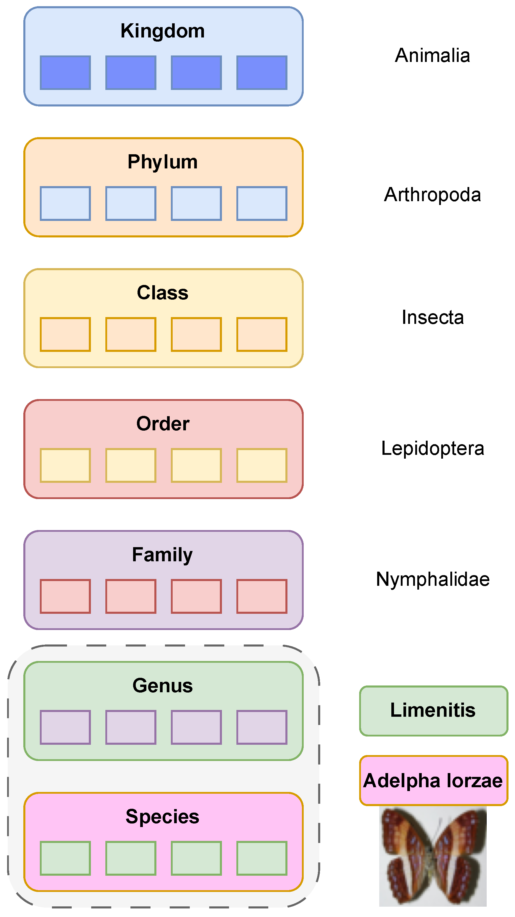
Figure 2.
Dataset example
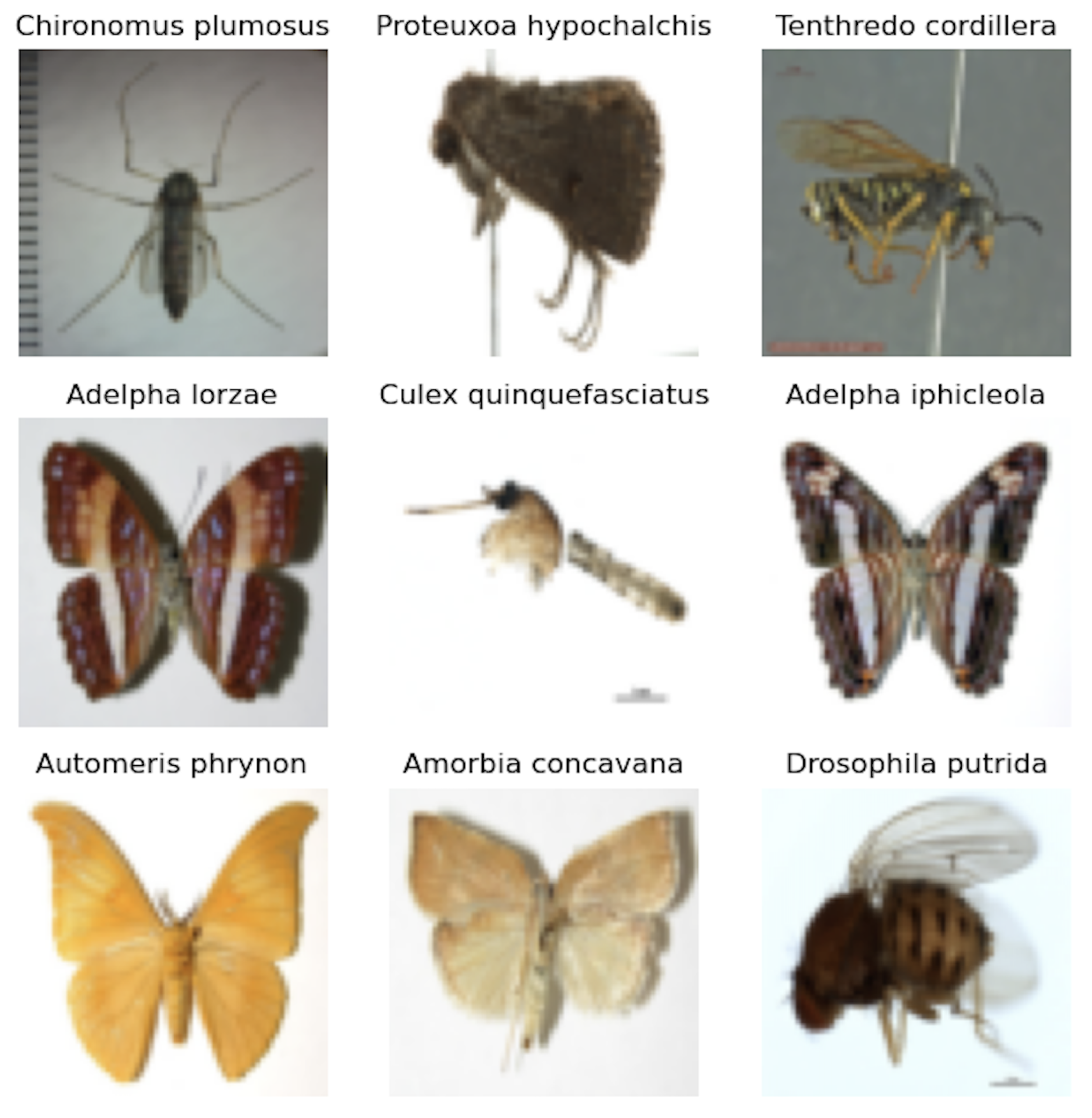
Figure 3.
Comparison of convolution with convolution: I is the input of the convolution and K is the filter.
Figure 3.
Comparison of convolution with convolution: I is the input of the convolution and K is the filter.
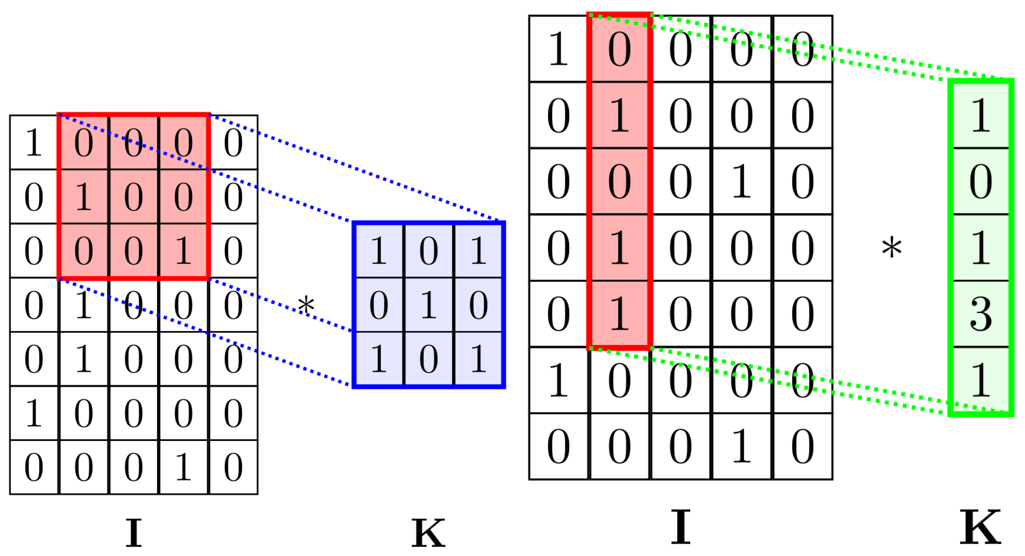
Figure 4.
Images generated by the ReACGAN.
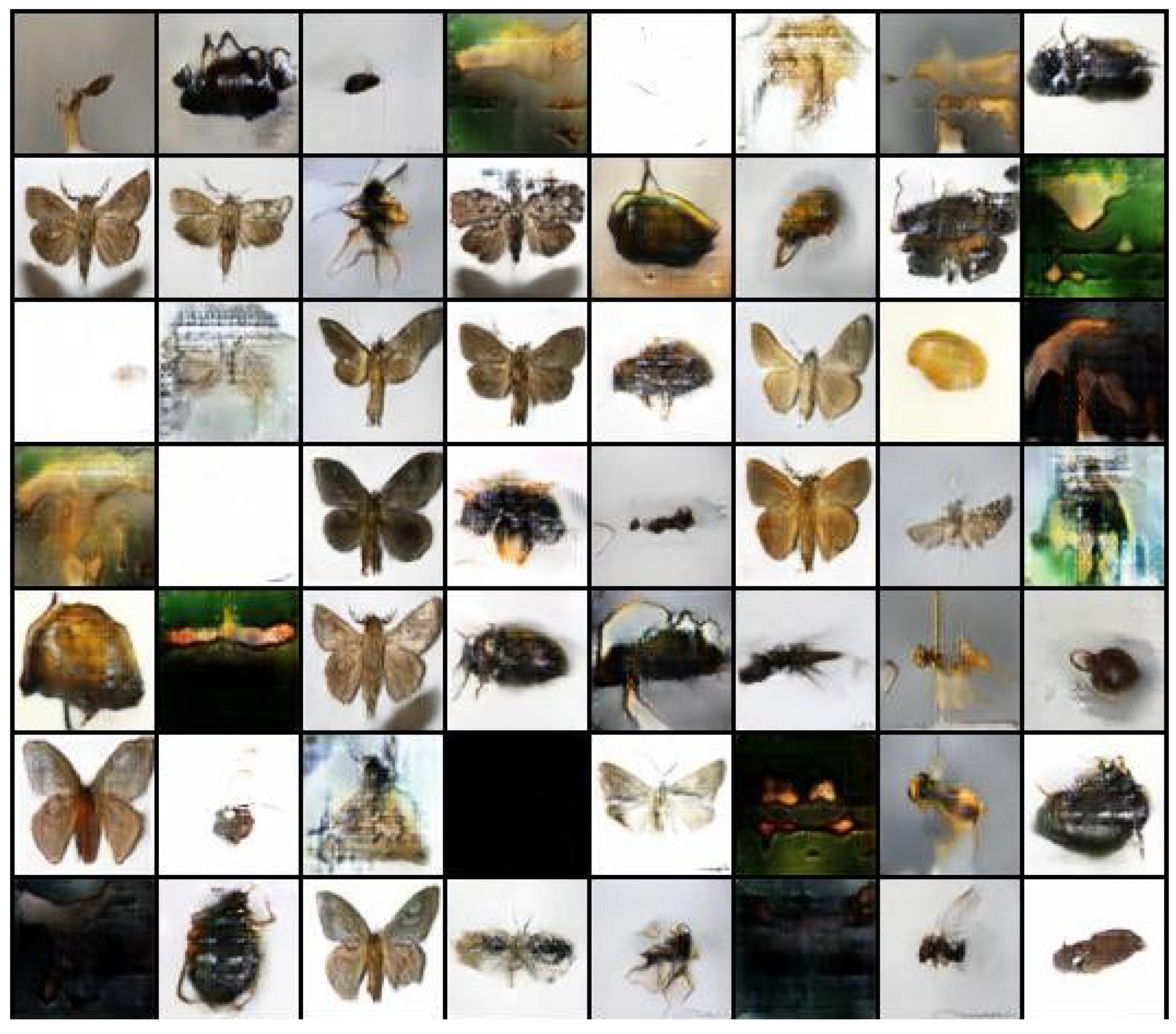
Figure 5.
DWTfilter
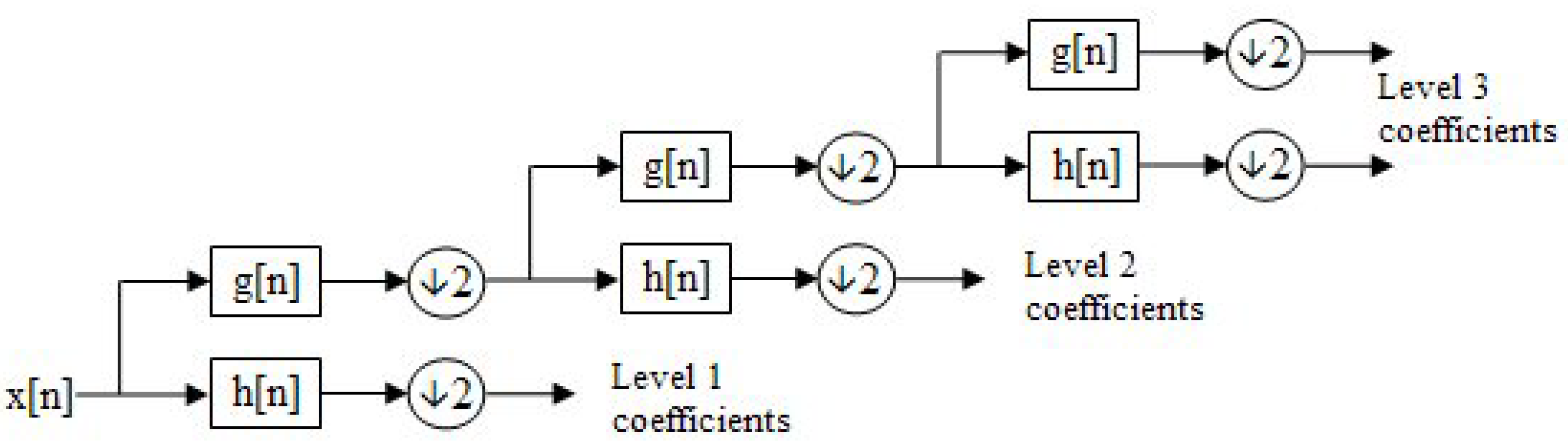
Figure 6.
(green line) vs Proposed ensemble (black line), species accuracy (x-axis) versus genus accuracy (y-axis) obtained by varying the rejection threshold .
Figure 6.
(green line) vs Proposed ensemble (black line), species accuracy (x-axis) versus genus accuracy (y-axis) obtained by varying the rejection threshold .
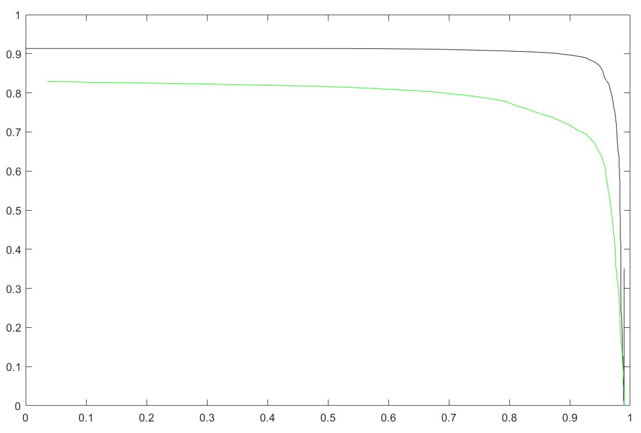

Table 1.
Differences in the collected dataset compared to [12], the columns Genera and Species report the number of classes of the samples.
Table 1.
Differences in the collected dataset compared to [12], the columns Genera and Species report the number of classes of the samples.
| Genera | Species | Samples | |
|---|---|---|---|
| [12] | 368 | 1040 | 32848 |
| Here | 371 | 1050 | 32424 |
Table 2.
Badirli Dataset.
| Badirli | Species | Genus |
|---|---|---|
| Bad | 98.21 | 81.95 |
| 98.65 | 71.85 | |
| [31] | 99.47 | 83.22 |
| 99.20 | 80.23 | |
| 99.22 | 81.26 | |
| 99.17 | 76.57 | |
| + | 99.40 | 81.92 |
| eDNA | 98.74 | 87.20 |
| Proposed | 99.47 | 87.74 |
Table 3.
New Insects Dataset, Section 2.1.
Table 3.
New Insects Dataset, Section 2.1.
| New Insects | Species | Genus |
|---|---|---|
| [31] | 99.05 | 84.02 |
| 99.16 | 79.07 | |
| 98.21 | 82.01 | |
| 98.05 | 65.05 | |
| 99.00 | 83.67 | |
| 98.83 | 75.08 | |
| 98.54 | 82.98 | |
| 99.12 | 83.85 | |
| + | 99.15 | 85.51 |
| eDNA | 98.48 | 88.49 |
| Proposed | 98.99 | 91.35 |
Table 4.
Unseen Dataset, Section 2.2.
Table 4.
Unseen Dataset, Section 2.2.
| Unseen | Genus |
|---|---|
| 23.85 | |
| 32.75 | |
| 46.82 | |
| 47.70 | |
| 30.38 | |
| 28.25 | |
| 42.73 | |
| + | 48.15 |
| eDNA | 33.36 |
| Proposed | 48.56 |
Table 5.
Beetle Dataset.
| Beetle | Species |
|---|---|
| [20] | 98.10 |
| [***] | 98.20 |
| 95.13 | |
| 90.48 | |
| 97.69 | |
| 97.69 | |
| — | |
| 62.72 | |
| 86.66 | |
| + | 98.03 |
| eDNA | 98.20 |
| Proposed | 98.51 |
Table 6.
Fish Dataset.
| Fish | Species |
|---|---|
| [20] | 96.30 |
| 94.75 | |
| 91.73 | |
| 95.70 | |
| 95.61 | |
| — | |
| 93.22 | |
| 92.82 | |
| + | 96.83 |
| eDNA | 96.75 |
| Proposed | 97.03 |
Disclaimer/Publisher’s Note: The statements, opinions and data contained in all publications are solely those of the individual author(s) and contributor(s) and not of MDPI and/or the editor(s). MDPI and/or the editor(s) disclaim responsibility for any injury to people or property resulting from any ideas, methods, instructions or products referred to in the content. |
© 2025 by the authors. Licensee MDPI, Basel, Switzerland. This article is an open access article distributed under the terms and conditions of the Creative Commons Attribution (CC BY) license (http://creativecommons.org/licenses/by/4.0/).
Copyright: This open access article is published under a Creative Commons CC BY 4.0 license, which permit the free download, distribution, and reuse, provided that the author and preprint are cited in any reuse.


