CO₂ Emission Prices, Freight Costs, and Inflation: Some Early Evidence

1. Introduction

Shipping serves most world transportation of goods since it accounts for approximately the 85% of international trade [1]. At the same time, according to a recent study by Wang et al. [2], ocean-going vessels are responsible for 17.2% of the global gas emissions that are responsible for the climate change of the last 20 years. Given the importance of shipping in world trade and the recent developments concerning climate change, the industry has come under scrutiny by policymakers regarding the environmental performance of vessels. Under this light, policymakers have enacted a specific tax that aims to penalize heavily emitting vessels and support the shift to alternative fuels. The CO2 emissions tax has been implemented to the industry since January 2023 and now is in its initial years of its operation. The latter comes as a consequence to the IMO strategies1 to reduce Greenhouse Gas (GHG) emissions that have started in July 2011, during the 62nd Meeting of the Marine Environment Protection Committee [3].

Carbon dioxide (CO₂) emissions, primarily stemming from the combustion of fossil fuels such as coal, oil, and natural gas, are the leading contributors to anthropogenic climate change​ [4]. These emissions trap heat in the atmosphere, exacerbating global warming, which has cascading effects on ecosystems, weather patterns, and global economies [5,6]. In response to these challenges, regulatory measures, including the introduction of tariffs on CO₂ emissions in shipping from 2023, aim to incentivize cleaner practices. These measures, though necessary for achieving sustainability, have significant implications for the global supply chain, potentially increasing transportation costs and influencing inflationary pressures [7]. The introduction of CO₂ emissions taxes in the shipping sector represents a critical step toward decarbonizing one of the world's most significant transportation industries. By imposing a financial cost on greenhouse gas emissions, these taxes aim to encourage shipping companies to adopt cleaner technologies, optimize fuel usage, and consider transition to alternative energy sources, while addressing the environmental and economic challenges posed by global warming [8].

As with any given tax or tariff, one expects that higher costs will have an impact on the whole supply chain of products given the scrolling effect between the producers and the final consumers. Thus, in this paper, we examine whether there has been any pass-through of the taxation from ship-owners to the consumer. Given that this would imply an increase in prices, one expects a corresponding increase in the overall price level via this inflationary channel. As such, one would expect that the CO2 emissions tax would leave the shipping industry intact, while the cost burden will have been rolled over to the consumers. However, our results provide alternative insights into the matter.

In particular, using a Bayesian Vector Autoregression (BVAR) model, we find that higher CO2 allowance prices do not have an impact on the economy via the shipping channel, since inflation does not seem to be affected by such a shock. The reason is that CO2 prices are not passed on to shippers, and hence they do not impact the real economy, unlike a generic freight rate shock. On the contrary, CO2 allowance prices have a negative effect on Brent oil prices, which not only counters their impact but also allows for a mild, short-term increase in earnings. As such, on the basis of the currently available data, the results underline that while the green transition can potentially affect the price level, this is unlikely to take place via the shipping channel.

Following this introduction, the remainder of this paper is organized as follows: section 2 provides a review of the literature on the issue, section 3 describes the methodology and the data used, section 4 discusses the empirical results obtained, and section 5 concludes on the findings.

2. Literature Review

Recent research highlights the growing importance of decarbonization in the shipping industry as a response to global calls for CO2 reduction and sustainable practices in freight transportation. Maritime transportation is responsible for around 3% of global CO2 emissions [8], with projections indicating potential increases due to the rise in global trade volumes and limited regulatory enforcement [9]. Also, the emissions of manufacturing process of exporting goods can reach a percentage of around 26% for some countries [10]. To address this, industry stakeholders have explored various technical and operational strategies, emphasizing alternative fuels, energy-efficient technologies, and regulatory frameworks.

Many studies focus on identifying cost-effective measures for emissions reduction, particularly through technological advancements and operational adjustments. Doukas et al. [11] examine innovative container designs and operational measures, such as optimizing speed, which offer emissions reductions without significant infrastructure changes​. Tran and Lam [12], have highlighted the importance of slow steaming benefits both reducing fuel consumption and emissions, though it presents challenges related to longer transportation periods and a higher cost when it comes to inventories.

A transition toward eco-friendly fuels has been identified as a crucial strategy for achieving low-carbon maritime transport. Hellström et al. [13] have provided evidence that there is not a one-size-fits-all measure when it comes to the reduction of GHG emissions in shipping. More precisely, they show that different fuels (i.e. methanol, ammonia, hydrogen and batteries) can serve different shipping segments. The latter is not only believed by the academia but also executive managers are of the opinion that green management and green efficiency contribute to controlling the impact of pollution with practical effects on economic sustainability [14]. Additionally, the tax and the financial incentives and environmental sustainability regulations indicate the relevance of the pollution impact and sustainable economy. Finally, since taxation of CO2 emissions also has emerged as a strategic option by the IMO, and the research of Cheaitou et al. [15] has shown that similar tax policies at the Northern Sea Routes have influenced route attractiveness and driven shifts in fuel usage.

The "Fit for 55" policy package of the European Union, which expands the Emissions Trading System (EU ETS) to encompass the shipping sector, underscores the economic implications of regulatory actions on shipping expenses and logistical choices. Vierth et al. [16] analyze various scenarios, demonstrating that although heightened costs promote the utilization of larger vessels, they could also result in shifts between transport modes if CO₂ costs continue to be externalized for smaller vessels. Xing et al. [9] further examine the implications of the International Maritime Organization's (IMO) targets for 2030 and 2050, emphasizing that the successful execution of these goals relies heavily on both the adoption of new technologies and the fostering of international collaboration.

Research continues to expand on the interdisciplinary approach needed for decarbonizing maritime freight transport. Singh et al. [17] emphasize the significance of digital technologies, including big data and blockchain, in enhancing logistics and minimizing emissions. These innovations facilitate operational efficiency, especially in the management of intricate supply chains and the reduction of empty container repositioning, which is a substantial factor in both emissions and operational expenses. Collectively, these studies reveal that while multiple decarbonization pathways exist, each approach involves trade-offs. The choice of measures must consider vessel types, route characteristics, and regulatory constraints. Future research should address the economic and policy barriers hindering widespread adoption of green technologies, as well as develop standardized frameworks that facilitate international compliance and sustainable growth in maritime logistics.

3. Methodology

As already discussed, this paper uses a Bayesian Vector Auto-Regression (BVAR) model [18] in which $y_{i,t}$ denotes a matrix with i variables relevant to the topic we intend to study. The BVAR representation is similar to the standard Vector Autoregression [19] and can be specified as:

$${\Delta \mathit{y}}_t=\alpha +{\sum }_{j=1}^k{\beta }_{1j}{\Delta \mathit{y}}_{t-j}+{\sum }_{j=1}^k{\beta }_{2j}{\Delta \mathit{x}}_{t-j}+{\epsilon }_t,{\epsilon }_t~N(0,\mathit{\Sigma })$$

(1)

where $y_t$ is a vector of endogenous variables and $x_t$ is a vector of exogenous variables, Δ is the quarter-over-quarter difference operator, j is the appropriate lag length and ${\epsilon }_t$ denotes the vector of serially and mutually uncorrelated structural innovations, with variance-covariance matrix Σ. In our case, no exogenous variables have been used, hence the formulation simplifies to:

$${\Delta \mathit{y}}_t=\alpha +{\sum }_{j=1}^k{\beta }_{1j}{\Delta \mathit{y}}_{t-j}+{\epsilon }_t,{\epsilon }_t~N(0,\mathit{\Sigma })$$

(2)

Similar to the standard VAR setup, ${\beta }_j$ are the appropriate coefficients related with lag j of the vector of dependent variables. For this model, vector $y_t$ includes the basic variables that are usually employed in the shipping literature, notably, Brent oil price, Eurostoxx, World Fleet, Freight Rates, Inflation, and Euribor. Our main contribution here is the inclusion of the CO2 emission allowance prices, for the first time in the literature. Following the standard in the literature, all variables are transformed into natural logarithms.

There are specific reasons concerning the use of the said variables in our analysis. First, the CO2 emissions allowance price is expected to have a positive effect on freight rates. The idea is that if shipowners have to use emission allowances as part of their IMO obligations, then they will likely pass the cost on to the shipper. As such, they will demand higher freight rates to cover for the additional cost of operations, as imposed by the regulations.

Concerning the other variables, Brent oil prices serve as a proxy for the cost of operating vessels, given that fuel costs can account for up to two-third of total costs [20,21]. As a result, higher Brent oil prices are expected to be passed on to shippers, suggesting that this would raise overall freight costs. Similarly, World Fleet serves as a proxy for the total supply of shipping, with the expected relationship between that and freight rates seen to be negative [22,23].

On the other hand, the Eurostoxx index serves as a proxy of European macroeconomic conditions, given the difficulty of obtaining real GDP data at a higher frequency. A higher stock market index suggests that demand is increasing, hence one would expect freight rates to rise, i.e. a positive relationship between stock prices and freight rates.

With regards to the other two macroeconomic variables, we include inflation (at constant prices to avoid any taxation problems) in order to be able to examine whether CO2 emissions have had any effect on it. However, given that inflation is known to have a negative relation with interest rates, and that inflation is the main variable in a central bank’s reaction function, we also need to include a proxy for interest rates. As such, we opt for the most popular metric, the 3-month Euribor contract. Finally, with regards to shipping-related variables, we employ the Baltic Dry Index (BDI) and shipowner earnings. The BDI is a proxy for global freight rates and has been highly popular in the literature, with most researchers employing it when it comes to examining the shipping sector [24] . An increase in freight rates after an increase in CO2 allowance prices would imply that the emissions cost is passed on to the shippers. On the other hand, we use shipowner earnings to examine whether owners choose to reduce their earnings in response to a change in emissions cost. If this is the case, then we expect a negative relationship between CO2 emission allowance prices and shipowner earnings.

Given that the IMO regulations have only been implemented in 2023, we are limited with regards to our sample size. As we cannot use any data for CO2 prior to 2023 as these were not binding for shipping, we force our sample to start in January 2023 and use the latest available data (August 2024) as our end sample date. With regards to data sources, the inflation series was obtained from Eurostat, while the Euribor and Eurostoxx data was obtained by the ECB’s Statistical Data Warehouse. Brent oil prices were collected from the Federal Reserve of St.Louis Database (FRED), while the Baltic Dry Index, World Fleet, and CO2 series were obtained from Clarksons research.

As the reader can observe, the biggest limitation of this study lies in the short sample size. However, we note that the reason behind the use of the BVAR model lies in its ability to perform well in small samples. As recent research has demonstrated (Li et al., 2024), BVAR models offer more precision in short and long horizons, also with regards to impulse response functions, which are employed to gain structural insights into the relationships. Naturally, regardless of the estimation method (Bayesian or frequentist), the same statistical properties need to hold: the variables need to be stationary, and the model needs to satisfy the stability criteria. To this end, stationarity tests which confirm that all the included variables are stationary, while the selected model is stable.

Concerning the estimation methodology, the literature has shown that the original Litterman [18] Minnesota prior necessitates some unwanted assumptions, namely that of an a priori known variance-covariance matrix. That assumption comes at the cost of imposing a Kronecker structure on the prior distribution, which creates, for each equation, a dependence between the variance of the residual term and the variance of the VAR coefficient (see [25]. In other words, such an assumption can potentially imply that the prior is set too tightly, and thus dominate any information stemming from the data.

To avoid this undesirable assumption, we employ a non-informative normal inverse-Wishart prior, as in Uhlig [26]. As such, the prior distribution is specified such that, $\beta ~N\left({\beta }_0,{\Omega }_0\right)$. The literature defines the ${\beta }_0$ and ${\Omega }_0$ using the Minnesota ${\beta }_0$ vector, with ones in the first lag of each endogenous variable and zero for further lags and cross-variable lag coefficients [25], a convention we follow in this paper as well. Similarly, ${\mathsf{\Omega }}_0$ also follows the Minnessota covariance matrix.

Following Koop and Korobilis [27], if the variables are in growth rates, then they advocate that the prior mean for the first lag is set to zero, while if the variables are in levels the prior mean could be set to 1 in order to capture any random walk behaviour. In our case, even though our variables are stationary, we set the first lag prior at 1, given that we do not want the prior value to overly restrict the model. Following this, Koop and Korobilis [27] also set the values for the prior covariance matrix to stand at ${\mathsf{\alpha }}_1/{\mathrm{r}}^2$for coefficients on own lags (r), where r = 1, … , p, implying that the prior value of the coefficient goes to zero as the number of lag s increases. For cross-coefficients the variance becomes ${\mathsf{\alpha }}_2{\mathsf{\sigma }}_{\mathrm{i}\mathrm{i}}/{\mathrm{r}}^2{\mathsf{\sigma }}_{\mathrm{j}\mathrm{j}}$.

In the independent Normal-Wishart case, the generic nature of the prior allows the researcher to use any prior covariance values. To make it computationally easier, the covariance matrix also follows the Minnesota prior, with the values specified as above. While a non-informative prior can also be used by setting all prior values to zero, we do not employ this setup, given that it is seldomly used in the literature. Following this, a Gibbs sampler is used for the estimation, which allows the researcher to obtain random draws from the unconditional posterior distributions of the parameters of interest.

As again, this is standard in the literature on Bayesian applications, we employ 10,000 iterations for the convergence of the algorithm, with the first 1,000 to be discarded as the burn-in sample. Standard hyperparameter values are used, i.e. an autoregressive coefficient of 0.8, tightness of 0.1, cross-variable weighting of 0.5, lag decay of 1 and 100 for the exogenous variable tightness. A lag length of two was selected based on the log-likelihood function results.

With regards to the identification method, like all other VAR model setups, regardless of their estimation method, we employ a Cholesky ordering for the impulse responses. As it is well-known, this implies that variable ordering also plays a role in the estimation results. In our case, the ordering suggests that, since CO2 and Brent prices are obtained at the global level, they are ordered first. Then, we order the fast-moving stock market variable (EuroStoxx 50), followed by inflation, and the Euribor rate. Given that the decisions to buy or sell vessels are conditional on the aforementioned variables, world fleet is ordered next, while the BDI is ordered last since it is affected by all of the previous variables. Naturally, a change in the variable order can have a potential effect on the results, however, the effects we observe are only quantitative and not qualitative.

For robustness purposes, we also provide a specification where we exclude Brent prices and the Euribor rate, in order to have a more parsimonious model. The impulse response functions we observe are similar to the ones from the full model, thus supporting the results and providing a useful robustness check. The results from the estimation are presented in the next section.

4. Empirical Results

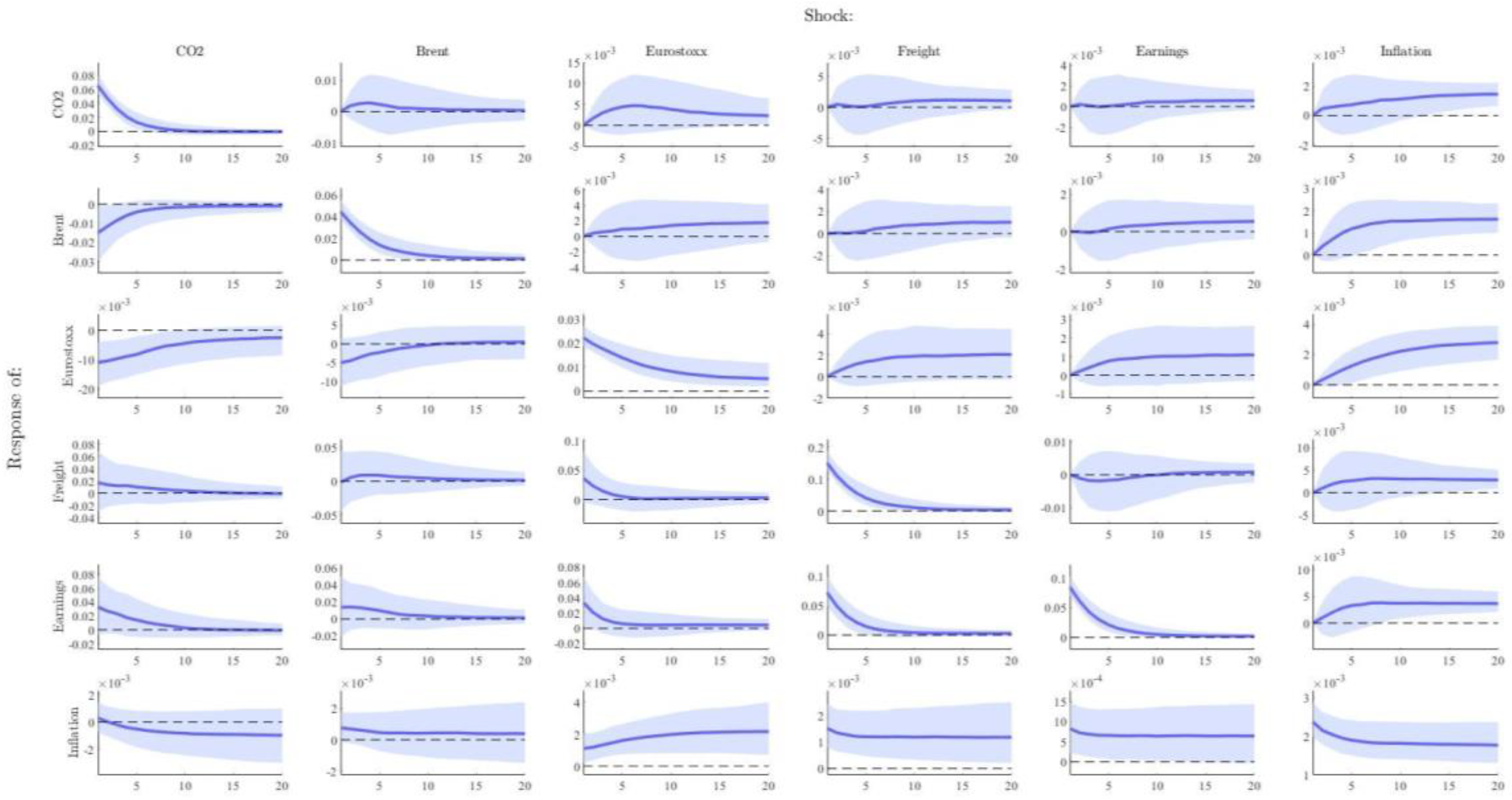
Figure 1 provides the results from the above-specified model. The main thrust of the results from this model appears in the first column of the figure. As per the reactions, a one standard deviation (transitory) shock on CO2 emission allowance price (approximately 7%) leads to Brent oil decline by around 1.5%, with the reaction lasting for a few months before moving to zero. The reaction highlights that the two are complementary, suggesting that higher allowance prices are likely discounted in the price of oil instead of being passed on to shippers.

This is confirmed by the rest of the variables, given that freight rates do not register a significant response, suggesting that no pass-through is found. However, earnings appear to increase, even though the reaction is significant for a couple of periods. On the basis of the above discussion, this does not appear to be the outcome of higher freight rates, but the result of lower Brent oil prices, which account for more than 60% of total vessel operating costs. Thus, despite the increase in CO2 allowance prices, shipowner earnings increase, as a result of this counterbalancing effect stemming from lower Brent oil prices. As the figure suggests, a 1% increase in the cost of emission allowances is translated into a 0.15% decrease of Brent oil prices, and a 0.4% increase in overall earnings. The effect is strong enough to also counterbalance the impact from lower stock prices, even though the shock reaction is relatively small.

Most importantly, the inflation reaction is also insignificant, suggesting the absence of a pass-through from CO2 allowance prices to prices via the shipping channel. This result suggests that while the cost of green transition can be, temporarily, inflationary for the overall economy, this will not come via higher shipping rates, which do not appear to be affected.

The remaining columns showcase the reliability of the model estimates, on the basis of the IRFs. In particular, the second column shows that there exists no bi-directional causal effect between Brent prices and CO2 allowance prices, as the latter does not respond to a shock in the former. Furthermore, it appears that the reaction of all other variables is as expected, with freight rates and earnings rising mildly, suggesting that oil price changes are being passed on to the shipper. As expected, core inflation does not respond to oil price changes.

The third column shows the responses from a shock in the Eurostoxx index. Higher stock prices have the expected positive and significant effect on freight rates, as also evidenced by the literature on the topic. For such a shock, higher freight rates, given that they are caused by a more favourable macroeconomic environment, appear to have a positive effect on earnings, again highlighting the effects that the broader macroeconomic environment can have on the shipping industry’s wellbeing. As also expected, expected positive changes in the macroeconomic environment, combined with higher freight rates, tend to be inflationary, even though the impact is relatively low, at 0.2%.

The bi-directional causality between freight rates and inflation is emphasised further in the fourth column: higher freight rates have a positive effect on both earnings and inflation, with the reaction standing at around 0.15% to a 7% shock. To put this in perspective, a 1% increase in freight rates would cause roughly a 0.02% increase in inflation, with a 100% increase (as also occurred in 2022) having a 2% impact on core inflation. Interestingly, a transitory shock to freight rates has a permanent effect on inflation, with the effect remaining stable for around 20 periods. The relationship between the shipping industry and inflation is further evidenced in the fifth column, where higher earnings appear to cause a permanent increase in inflation, even though to a much lower extent (0.01% per 1% shock).

In the final column, the responses from a shock in inflation can be observed. As the figure suggests, the impact from higher inflation is positive on CO2 allowance prices, Brent oil and the overall stock market, with a medium-run positive effect on freight rates and earnings. In particular, a 1% shock in inflation causes an approximately 1% increase in CO2 allowance prices and the price of oil, while the stock market increases by around 1.5%. The shipping variables react by a higher order of magnitude, reporting a 4% increase in freight rates and approximately a similar increase in earnings. Interestingly, the response does not become significant until a year after the shock, a result in line with Michail and Melas [21], who report that ship-owners react with a lag to non-shipping information like demand.

Overall, the results suggest that higher CO2 allowance prices do not have an impact on the economy via the shipping channel, since inflation does not seem to react in such a shock. The reason is that CO2 prices are not passed on to shippers, and hence they do not impact the real economy, unlike a generic freight rate shock. On the contrary, CO2 allowance prices have a negative effect on Brent oil prices, which not only counters their impact but also allows for a mild, short-term increase in earnings. As such, on the basis of the currently available data, the results underline that while the green transition can potentially affect the price level, this is unlikely to take place via the shipping channel.

5. Conclusions

Recent research highlights the growing importance of decarbonization in the shipping industry as a response to global calls for CO2 reduction and sustainable practices in freight transportation. Given that maritime transportation is responsible for around 17.2% of the global gas emissions that are responsible for the climate change of the last 20 years, with projections indicating potential increases due to the rise in global trade volumes and limited regulatory enforcement, imposing emissions limits had become a sine qua non. Under this light, policymakers have enacted a specific tax that aims to penalize heavily emitting vessels and support the shift to alternative fuels. The CO2 emissions tax has been implemented in the shipping industry in January 2023 and now is in its initial years of its operation.

As with any tax, expectations are that the higher costs will have an impact on the whole supply chain, as the extra cost will be passed through from ship-owners to the end consumer. As such, one would expect that the CO2 emissions tax would leave the shipping industry intact, while the cost burden will have been rolled over to the consumers, resulting in an increase in overall inflation. However, our results, using a Bayesian Vector Autoregression (BVAR) model, suggest differently. We find that higher CO2 allowance prices do not have an impact on the economy via the shipping channel, since inflation does not seem to react in such a shock. The reason behind this is that CO2 prices are not passed on to shippers, and hence they do not impact the real economy, unlike a generic freight rate shock. On the contrary, CO2 allowance prices have a negative effect on Brent oil prices, which not only counters their impact but also allows for a mild, short-term increase in earnings. As such, on the basis of the currently available data, the results underline that while the green transition can potentially affect the price level, this is unlikely to take place via the shipping channel. Our results are in-line with the broader bibliography that shows that the reduction of the Co2 emissions will contribute negatively to the world economy [6]

Policy wise, our results show that while the Co2 emission carbon tax on the shipping industry has been implemented quite recently, this has not affected the cost of goods as expressed by inflation. Given the latter, one can suggest that shipping acts as a good mediating industry on the one hand to minimize the Co2 emissions and on the other hand not to hamper the economic growth. In line with the previous literature [24,28,29,30,31,32], our research shows the serious economic and policy impact that the maritime industry can have on the world economy and the importance that should be given to the industry by the policy makers. Naturally, the main limitation of our research is the shortage of data. Thus, future research is needed on this front when more data will be available.

References

- UNCTAD Review of Maritime Transport 2023; New York, 2023;
- Wang, X.-T.; Liu, H.; Lv, Z.-F.; Deng, F.-Y.; Xu, H.-L.; Qi, L.-J.; Shi, M.-S.; Zhao, J.-C.; Zheng, S.-X.; Man, H.-Y.; et al. Trade-Linked Shipping CO2 Emissions. Nat Clim Chang 2021, 11, 945–951. [CrossRef]
- Joung, T.H.; Kang, S.G.; Lee, J.K.; Ahn, J. The IMO Initial Strategy for Reducing Greenhouse Gas(GHG) Emissions, and Its Follow-up Actions towards 2050. Journal of International Maritime Safety, Environmental Affairs, and Shipping 2020, 4, 1–7. [CrossRef]
- Yoro, K.O.; Daramola, M.O. CO2 Emission Sources, Greenhouse Gases, and the Global Warming Effect. In Advances in Carbon Capture: Methods, Technologies and Applications; Elsevier, 2020; pp. 3–28 ISBN 9780128196571.
- Montzka, S.A.; Dlugokencky, E.J.; Butler, J.H. Non-CO 2 Greenhouse Gases and Climate Change. Nature 2011, 476, 43–50. [CrossRef]
- Mardani, A.; Streimikiene, D.; Cavallaro, F.; Loganathan, N.; Khoshnoudi, M. Carbon Dioxide (CO2) Emissions and Economic Growth: A Systematic Review of Two Decades of Research from 1995 to 2017. Science of the Total Environment 2019, 649, 31–49. [CrossRef]
- Davis, S.J.; Caldeira, K.; Matthews, H.D. Future CO2 Emissions and Climate Change from Existing Energy Infrastructure. Science (1979) 2010, 329, 1330–1333. [CrossRef]
- Wu, R.; Li, M. Optimization of Shipping Freight Forwarding Services Considering Consumer Rebates under the Impact of Carbon Tax Policy. Ocean Coast Manag 2024, 258. [CrossRef]
- Xing, H.; Spence, S.; Chen, H. A Comprehensive Review on Countermeasures for CO2 Emissions from Ships. Renewable and Sustainable Energy Reviews 2020, 134. [CrossRef]
- Yunfeng, Y.F.; Laike, Y.K. China’s Foreign Trade and Climate Change: A Case Study of CO2 Emissions. Energy Policy 2010, 38, 350–356. [CrossRef]
- Doukas, H.; Spiliotis, E.; Jafari, M.A.; Giarola, S.; Nikas, A. Low-Cost Emissions Cuts in Container Shipping: Thinking inside the Box. Transp Res D Transp Environ 2021, 94. [CrossRef]
- Tran, N.K.; Lam, J.S.L. Effects of Container Ship Speed on CO2 Emission, Cargo Lead Time and Supply Chain Costs. Research in Transportation Business and Management 2022, 43. [CrossRef]
- Hellström, M.; Rabetino, R.; Schwartz, H.; Tsvetkova, A.; Haq, S.H.U. GHG Emission Reduction Measures and Alternative Fuels in Different Shipping Segments and Time Horizons – A Delphi Study. Mar Policy 2024, 160. [CrossRef]
- Felício, J.A.; Rodrigues, R.; Caldeirinha, V. Green Shipping Effect on Sustainable Economy and Environmental Performance. Sustainability (Switzerland) 2021, 13. [CrossRef]
- Cheaitou, A.; Faury, O.; Etienne, L.; Fedi, L.; Rigot-Müller, P.; Stephenson, S. Impact of CO2 Emission Taxation and Fuel Types on Arctic Shipping Attractiveness. Transp Res D Transp Environ 2022, 112. [CrossRef]
- Vierth, I.; Ek, K.; From, E.; Lind, J. The Cost Impacts of Fit for 55 on Shipping and Their Implications for Swedish Freight Transport. Transp Res Part A Policy Pract 2024, 179. [CrossRef]
- Singh, S.; Dwivedi, A.; Pratap, S. Sustainable Maritime Freight Transportation: Current Status and Future Directions. Sustainability (Switzerland) 2023, 15. [CrossRef]
- Litterman, R.B. Forecasting With Bayesian Vector Autoregressions—Five Years of Experience. Journal of Business & Economic Statistics 1986, 4, 25–38. [CrossRef]
- Sims, C.A. Macroeconomics and Reality. Econometrica 1980, 48, 1. [CrossRef]
- Stopford, M. Maritime Economics; 3rd ed.; Routledge: New York, 2013; ISBN 9781134742677.
- Michail, N.A.; Melas, K.D. Containership New-Building Orders and Freight Rate Shocks: A “Wait and See” Perspective. Asian Journal of Shipping and Logistics 2023, 39, 30–37. [CrossRef]
- Michail, N.A.; Melas, K.D. Covid-19 and the Energy Trade: Evidence from Tanker Trade Routes. The Asian Journal of Shipping and Logistics 2021, 1–30. [CrossRef]
- Michail, N.A.; Melas, K.D. Sentiment-Augmented Supply and Demand Equations for the Dry Bulk Shipping Market. Economies 2021, 9, 171. [CrossRef]
- Michail, N.A. World Economic Growth and Seaborne Trade Volume: Quantifying the Relationship. Transp Res Interdiscip Perspect 2020, 4, 100108. [CrossRef]
- Dieppe, A.; Legrand, R.; van Roye, B. The BEAR Toolbox; ECB Working Paper; European Central Bank, 2016;
- Uhlig, H. What Are the Effects of Monetary Policy on Output? Results from an Agnostic Identification Procedure. J Monet Econ 2005, 52, 381–419. [CrossRef]
- Koop, G.; Korobilis, D. Bayesian Multivariate Time Series Methods for Empirical Macroeconomics. Foundations and Trends in Econometrics 2009, 3, 267–358. [CrossRef]
- Kilian, L. Not All Oil Price Shocks Are Alike: Disentangling Demand and Supply Shocks in the Crude Oil Market. American Economic Review 2009, 99, 1053–1069. [CrossRef]
- Michail, N.A.; Melas, K.D. Geopolitical Risk and the LNG-LPG Trade. Peace Economics, Peace Science and Public Policy 2022, 28, 243–265. [CrossRef]
- Michail, N.A.; Melas, K.D.; Cleanthous, L. The Relationship between Shipping Freight Rates and Inflation in the Euro Area. International Economics 2022, 172, 40–49. [CrossRef]
- Michail, N.A.; Melas, K.D.; Batzilis, D. Container Shipping Trade and Real GDP Growth: A Panel Vector Autoregressive Approach. Economics Bulletin 2021, 41, 304–315. [CrossRef]
- Kilian, L.; Nomikos, N.; Zhou, X. Container Trade and the U.S. Recovery. Int J Cent Bank 2023, 19, 417–450. [CrossRef]
Figure 1.
Full Model Estimates.