
Submitted:
30 December 2024
Posted:
31 December 2024
You are already at the latest version
Abstract
This paper proposes a new disorder detection method CCF-AE for dynamic plant based only on its input-output relation using cross-correlation function and neural network autoencoder. CCF-AE method does not use the reference model of the dynamic object, but consider real-time behavior changes, given by input and output time series. The proposed method was used to detect disorder in the process of nonlinear pH-neutralization reaction, and the cumulative sum algorithm (CUSUM) was used in a comparative experiment. The experiment demonstrated better accuracy of the proposed method than the CUSUM algorithm. Also CCF-AE has more advantages in detecting disorder in the behavior of a complex nonlinear system.
Keywords:
disorder detection
; anomaly detection
; time series
; dynamic plant
; cross-correlation function
; neural network autoencoder
; cumulative sum algorithm
; pH neutralization reaction
1. Introduction
In increasingly complex industrial environment, the stable operation of automation control systems is crucial to ensuring improved production efficiency and product quality.
With the development of information technology, traditional control system design has gradually shifted from analog circuit architectures that rely on continuous signal processing to discrete-time control technology using intelligent algorithms. However, this change also brings with it new challenges—the increasing complexity of systems and the diversity of failure modes [1]. The complexity of systems highlights the problem of detection disorder and anomalies. The disorder is an unpredictable change of system parameters and the anomaly is a visible change of system behavior.
Disorder detection plays a vital role in modern automated control systems. It means a dynamic monitoring for the rapid detection of any behavior or pattern deviating from the regular operating state during system operation by analyzing real-time data, which is a so-called abnormal situation. The root of abnormal situation includes but is not limited to hardware performance degradation, operation errors, communication interruptions, etc., which may cause system instability or even crash.
The use of disorder detection technology helps to provide early warning and take preventive measures to prevent potential problems from worsening and maintain the efficient operation and safety of the entire system.
There are many situations that can lead to anomalies in the behavior of dynamic plants. Anomalies can occur individually or simultaneously due to defects in sensors, actuators or plants. However, in complex industrial systems, it is sometimes not easy to accurately monitor whether a certain performance status as a system health indicator is normal (i.e., whether it is a fault or not). For example, the degree of machine wear, changes in material properties, etc., these subtle changes may not be obvious at first, and we realize the problem only when they reach a certain level and cause system performance to degrade or fail. When monitoring multiple process parameters simultaneously, skilled operators often must make operating decisions based solely on their experience. Another reason for disorder in the behavior of dynamic plants can be changes in external influences on the system. This may be a change in both external conditions leading to a change in the dynamic characteristics of the system components, and the setpoint signal is different from expected.
In the maintenance of complex systems, fault detection faces severe challenges. First of all, real-time is crucial. The system must react and handle exceptions almost instantly and is sensitive to delays. Secondly, the data sent by the sensor may contain errors, such as inaccurate measurements or random fluctuations caused by changes in the external environment, which requires the algorithm to be highly reliable and resistant to interference. Besides, the continuous updating and adaptability of the model is also a challenge. The reference model in the anomaly detection process usually refers to the model used to identify and handle abnormal situations during system operation, which relies on the understanding of normal behavior and threshold setting. As the environment changes, the operating specifications of the system may change, such as new failure modes may appear, or operations considered to be normal previously may now become abnormal.
Modern approaches to disorder detection combine machine learning [2], big data analytics, and may incorporate cloud computing and IoT technology to enable data analysis using information not available in traditional control systems. From a practical perspective, the challenge for such approaches is to process large amounts of data efficiently in real time, while identifying disorder and ensuring the reliability of the detection algorithms so that they can cope with changing conditions and new causes of abnormal behavior in dynamic plants.
2. Background
Detecting a discord in the behavior of dynamic plants has been an active research area for many years [3,4].
Algorithms for detecting discord are usually based on real-time data. If the deviation between the plant output and the output of its reference model increases, an alarm or automatic adjustment mechanism is triggered. The simplest approach was to monitor the range of variation of the observed characteristics of the plant [5]. More complex approaches, such as the cumulative sum algorithm (CUSUM), are based on detecting the deviation of the statistical characteristics of the observed process from the normal behavior specified by the stochastic model of the norm. Typically, such a model implies the specification of the type and parameters of the distribution of the normal process.
In recent years, thanks to the significant enhancements in computer performance, disorder detection techniques using machine learning have gradually emerged, such as autoencoders [6,7]. As a powerful tool, the autoencoder can autonomously learn the basic structure and distribution of data and then reconstruct it. So, the data samples of normal working conditions will be mapped to similar ones, while the abnormal samples will not, resulting large difference between input and output vectors of autoencoder. Therefore, these points that deviate from the norm will be effectively identified, which not only improves the accuracy and reliability of anomaly detection, but also reduces the need for manual intervention, which helps to build a more intelligent and adaptive industrial monitoring system.
2.1. Model-Based Methods
Model-based disorder detection is a widely used technology in science and engineering. Its basic principle is to provide a mathematical description or algorithm for the behavior of the main characteristics of a system. This requires the use of mathematical formalisms to analyze the key physical principles and observed dependencies, often by constructing differential equations to characterize the dynamic processes. Model-based analysis is particularly effective when designing systems with clear structures and well-defined rules, such as simple mechanical devices in mechanical engineering or linear control systems in the field of automatic control, because models are easy to create and debug.
The task of detecting faults in systems and processes is to automatically identify dependencies between measured signals and subsequently detect changes in these dependencies. Based on the measured output signals of the plant and its reference model, modeling error values, estimated values of parameters, or estimated values of state variable values called features can be calculated. Changes or deviations in the detected features compared to normal features will lead to the analysis of symptoms [8,9].
A typical disorder detection scheme is shown in Figure 1.
This approach is based on the assumption that when the physical characteristics within the plant are slightly adjusted, the measured output signal will change accordingly. If this change deviates from the standard signal pattern estimated by the reference model, it will become obvious and can be identified as an abnormal situation. When using this approach, it is necessary to take into account that the reference model must repeat the behavior of the plant itself accurately and similarly respond to input effects to the plant.
However, when dealing with complex dynamic systems, such as chemical reaction processes or systems involving a large number of variables, building accurate reference model is often a difficult task, or even almost impossible. In such complex situations, detection methods that rely on building models of dynamic plants may no longer be applicable. Instead, an approach based on data analysis that does not require building accurate models of dynamic plants can be considered. Data-driven approaches are better suited to complex systems with high uncertainty due to the greater focus on analyzing empirical data rather than building detailed analytical mathematical models of a plant.
2.2. Data-Driven Methods
Data-driven anomaly detection, as a modern anomaly diagnosis strategy, based on a large amount of operational data as a primary resource. Its main idea is to collect data generated by the equipment under normal operating conditions, such as temperature, vibration, current and other measured parameters, and then use these time series to build a model. Data-based models can capture the evolution of plant performance over time and use it as the basis for distinguishing whether the plant is in normal condition.
The specific process includes data collection, pre-processing (cleaning, normalization, etc.), feature engineering (extracting key features that cause failures), and then training a model to define the normal operating mode of the plant.
When new data are fed into the model, if they deviate from the known data distribution significantly under normal operating conditions, an alarm will be triggered, indicating a potential failure. Data-driven methods such as machine learning can automatically learn patterns from observed historical data, better capture nonlinear correlations, and avoid relying on precise physical models, making them superior in dealing with nonlinear system problems.
Data-driven disorder detection technology is now widely used in various industrial processes including chemical industry [10], polymer manufacturing, microelectronics, steel industry, pharmaceutical processes, power distribution networks [11] and flow systems.
Especially in the last three decades, it has become one of the most fruitful areas of research and practice and an important tool for quality control [12,13].
2.2.1. Multivariate Statistical Process Control
Multivariate statistical process control in process monitoring emerged in the 1990s [14]. It uses statistical models to monitor manufacturing processes in real time by extracting key information from complex data sets. For example, statistical process control charts are used to compare the current state of a process to normal operating conditions. Most commonly, control charts are used to monitor the mean or deviation of selected variables that affect a process. Such as the Shewhart control chart [15], the CUSUM chart [16], the EWMA chart [17]. Each of the above types of control charts has its own advantages and disadvantages. The Shewhart control chart is a statistical tool based on past data fluctuations. It is designed with the assumption that samples are collected and analyzed continuously. When focusing only on existing test data, if improvements, anomalies, or slight changes in the process occur in a short period of time, the control chart may not immediately reflect these short-term changes due to the slow sample update, because it relies on historical means and standard deviations to determine the normal range. In short, control charts have a good ability to identify stable long-term trends, but they may not be sensitive enough for dynamic and fast-changing processes, especially those with frequent small adjustments. In contrast, the CUSUM and EWMA control charts are more sensitive in detecting small changes in the process because they use information from long-sequence samples. Therefore, for large-scale process failures that require an immediate response, the Shewhart control chart is an effective tool, but for continuous improvement or monitoring quality trends, other methods such as EWMA or CUSUM control charts may be needed to monitor the process in more detail. In practical applications, they are often used together to detect anomalies and evaluate process stability [18].
In general, multivariate statistical methods for discord detection use the typical Hotelling’s statistic and the Q statistic, which is also known as the squared prediction error. When the value exceeds a certain threshold, it means that the data points deviate from the normal pattern, i.e., deviations from the normal plane may be observed and, thus, discord is detected.
In the field of process control, principal component analysis (PCA) is one of the most popular statistical methods for extracting information from measured data [19]. The main step of PCA is to transform the original data into a low-dimensional linear independent space and residual space by linear projection. and Q statistics and their control limits are set in the corresponding space for fault detection.
However, when dealing with complex processes in fields such as industrial chemistry and biology, the use of PCA can be problematic if these processes involve significant nonlinear features such as periodic changes or adaptive responses within the system. Since the basic assumption of using PCA is that data changes are normally distributed and linearly related, its ability to detect nonlinear outliers will be weakened. For example, when outliers are generated by nonlinear relationships or the behavior of the data evolves over time rather than following a simple linear trend, a simple linear transformation of PCA may not accurately capture this outlier behavior of the system [20]. To overcome this shortcoming, several improved PCA schemes have been proposed. For instance, the paper [21] presented a nonlinear principal component analysis based on a five-layer neural network.
Partial least squares (PLS) is also a classic multivariate statistical analysis technique, which is used to establish a linear relationship between input and output. By building a model based on normal data in an a priori order, PLS can be implemented for forecasting and monitoring applications. Assuming that all measurements follow a normal distribution, and Q index are adopted as statistical indicators for detecting quality and non-quality defects [22]. In contrast to PCA, independent component analysis has been used for process monitoring by projecting correlated variables into an independent space without orthogonality constraints, making it more applicable to non-Gaussian processes [23]. Another method for dealing with non-Gaussian processes is the Gaussian mixture model, which fits multiple Gaussian models to approximate non-Gaussian data. It has been widely used for process monitoring in arbitrary data sets that do not follow a normal distribution [24,25].
2.2.2. Machine Learning Based Method
Machine learning models can automatically extract features and learn complex patterns from large amounts of data without manually developing complex hypotheses or hypothesis distributions. This is especially effective when dealing with non-linear and non-Gaussian distributed data. Some machine learning methods, such as support vector machines or artificial neural networks, have a certain noise resistance and the ability to handle isolated points. In recent years, there has been a growing interest in the application of artificial neural networks in fault detection and diagnostic systems [26,27,28].
The neural network replaces the analytical model describing the process under normal operating conditions. It must be trained to perform this task, and the training data can be collected directly from the process or from a simulation model that is as realistic as possible. Once the training is complete, the neural network can generate residuals that indicate anomalies. For example, the paper [29] described using the residuals between the output of a plant and its neural network model to detect anomalies in a real sugar evaporation process.
However, it is necessary to consider dynamics when modeling dynamic plants in automatic control systems using neural networks or detecting disorder in the behavior of a plant. In order to be able to record the dynamic behavior of the system, the neural network must have dynamic characteristics, such as recurrent neural networks. The paper [30] discusses a method for online detection of sensor disorder in substations based on a long-term short-term memory network and an adaptive threshold selection algorithm.
Using only a single fault detection algorithm may lead to false positive problems. In order to improve the accuracy and stability of detection, a common approach is to integrate multiple technical means, such as combining statistical analysis and machine learning methods. Such a comprehensive strategy can complement the advantages of each method, reduce the possibility of errors, and enhance the credibility of the final result.
The paper [31] proposed a process monitoring method using Gaussian mixture model and weighted kernel-independent component analysis, in which the Gaussian mixture model is used to estimate the probability of kernel-independent components, and the important kernel-independent components that dominate the process change are given a higher weight according to the estimated probability of collecting important information in the online disorder detection process.
The paper [32] adopted a method using automatic noise accumulation coding and K nearest neighbor (KNN) rule. An autoencoder with multi-level noise reduction is used to model nonlinear process data and automatically extract important features. The original nonlinear space is then mapped to the feature space and residual space using the multi-level denoising autoencoder. Two new statistics for detecting disorder in the above spaces are constructed by introducing a KNN rule with corresponding control limits determined by the kernel density estimation.
Although machine learning has shown great potential in the field of disorder detection, it still faces some challenges. In an industrial environment, continuous evolutionary processes may occur, such as equipment aging and changing failure modes. Traditional static anomaly detection methods can be difficult to account for these changes. And anomalies are often not a single pattern, but contain noise and unknown variables. If a model relies too heavily on a known data distribution, it may fail when it encounters new anomalies that were not previously noticed.
The main idea of this work is to use the cross-correlation function between the input and output of the plant as a characteristic of its nonlinear dynamics, combined with a neural network autoencoder, which helps detect when the plant operation shifts to a new pattern and when anomalies occur compared to the reference period of system operation. The proposed method does not rely on external reference signals, but directly analyzes real-time data from nonlinear dynamic systems, which can respond more quickly to real-time changes within the monitored plant. In addition, the autoencoder can dynamically learn the normal distribution of the data during the training process, thereby avoiding the subjectivity and variability caused by manual threshold setting.
For comparison, we conducted experiments using the proposed method and the cumulative sum algorithm respectively to detect disorder in the behavior of the same plant.
3. Method
3.1. Cross-Correlation Functions as Characteristics of a Dynamic System
As a statistical analysis tool, the cross-correlation function (CCF) describes the similarity between two signals or sequences, which is especially important for time series, since they reflect the relationship between previous and subsequent reference points. In the context of dynamic plants in control systems, it is possible to compare the time series measured by a sensor and the expected behavior of the plant [33].
If the system is not operating under normal conditions, for instance due to internal hardware or external disturbances, then the initially stable CCF may change, manifesting as a shift in the peak position, a reduction in amplitude, or a distortion in shape. This concept can be used to analyze whether the behavior of a plant in a dynamic system deviates from the normal mode.
For each successive time step t of the control system, the CCF value between the input signal and the output signal is calculated according to formula (1).
CCF is proposed as an effective feature representation for extracting local features of input-output time series of the control systems and subsequently feeding it into an autoencoder to capture key patterns in the data that may indicate abnormal behavior of the dynamic system.
In addition, by calculating the CCF, local similarities can be identified without changing the frequency characteristics of the signal, which helps the autoencoder learn an invariant representation of the data.
The calculation of continuous CCF needs to be converted into discrete form to match the data structure of the autoencoder input. In discrete time, for time series and , the CCF within a window with a width of samples starting from time series sample is calculated by formula (2):
The index indicates the position of the calculated CCF sequence in the time series, and the argument is the offset of one series that are relative to another, for which one discrete CCF value is calculated. Thus, the CCF at position can be viewed as a vector .
The set of CCF sequences describes the behavior of a dynamic system in response to an input signal over a period of time, forming a point cloud in a multidimensional space located in a certain area at different time periods under normal operating conditions.
Figure 2 shows an example of such a region in three-dimensional space, designated as .
When the input signal changes relative to the normal signal belonging to the region, the values in the CCF sequence will also change. We assume that the dynamic response of the system at time is represented by the point belonging to the normal region . Then, when the dynamic response changes at a certain moment , the CCF will be represented by the point in Figure 2.
A drift detected in the CCF vector space outside the region representing the normal behavior of the system means that at time either a change in the input signal or a change in the properties of the dynamic system has occurred. We call this phenomenon disorder.
3.2. Discord Detection Using Neural Network Autoencoder
In order to apply the proposed method, we need a method to memorize the CCF of the reference dynamic behavior of the process, as well as a way to find the difference between CCF and its norm. For this, we used a neural network autoencoder that can remember the CCF vectors from the training set and reproduces the memorized vectors. We trained the autoencoder by taking as input calculated from the input-output sequence of the process under normal conditions.
The autoencoder mainly consists of an encoder and a decoder, as shown in Figure 3. The encoder compresses the set of CCF vectors as input into a low-dimensional representation called a code vector. The decoder tries to recover the original set of CCF vectors from the code vector, where
Under normal circumstances, the output of the decoder should be as close as possible to the input. During training, the autoencoder learns the data distribution pattern of the set of CCF vectors calculated during the normal operation of the dynamic system and tries to minimize the reconstruction error, that is, the difference between the input and output data of the autoencoder. However, the decoding results of abnormal data will differ due to the abnormal performance after encoding.
When a disorder is detected in the behavior of a dynamic system, that is, the set of CCF vectors provided to the autoencoder input does not correspond to the prediction results of the trained model, and the actual loss exceeds a given threshold of the error in reconstructing the CCF .
3.3. Synthesis and Application of a Discord Detector
Figure 4 shows the scheme for synthesizing an autoencoder-based discord detector, and its steps are as follows:
Step 1: Data preparation. Collect a series of discrete time series of length at the input and output of a normally functioning dynamic system, i.e., input and output .
Step 2: Calculation of CCF. Calculate CCF from time series and and obtain a set of CCF vectors , describing the reference (normal) behavior of the dynamic system. Use index to specify the window number of the calculated CCF sequence, and its value is in the interval: .
Step 3: Training of the autoencoder. The training dataset of the autoencoder is a set of CCF vectors , which are the characteristics of the normal behavior of the dynamic system. The reconstructed CCFs by the autoencoder are denoted as . The reconstruction error is used to measure the difference between the reconstructed and original CCFs, where is usual Euclidean length.
Step 4: Determination of threshold. The maximum reconstruction error obtained during training is regarded as the trigger threshold, which indicates that the CCF series value has deviated from the expected.
The synthetic result of the disorder detector is the trained autoencoder and the disorder detection threshold .
To detect the disorder caused by the change in the dynamic response of the observation system , the obtained CCF-AE detector is put into the test. The scheme is shown in Figure 5 and is described below step by step:
Step 1: Collect a time series of consecutive input values and output values .
Step 2: Calculate the CCF from and, obtaining the vector .
Step 3: Calculate the reconstructed CCF value using the autoencoder and obtain the reconstruction error .
Step 4: Compare the reconstruction error with the threshold value . If means there is no disorder and the dynamic response of the system is similar to the responses known to the autoencoder, otherwise there is a disorder in the last interval of length indexed by and the observed system may behave inadequately.
Therefore, the dynamic characteristics represented by the CCF vector are used as input to the autoencoder to obtain the reconstruction error for evaluating the behavior of the dynamic system, which makes it possible to identify and localize disorders in the dynamic system.
3.4. Description of Comparative Experiments
To illustrate the proposed CCF-AE method, a neutralization reactor process model is used as a nonlinear dynamic plant, which provides the possibility of introducing new behavior patterns.
It is proposed to use the CCF vectors of the input and output time series of the observed nonlinear dynamic plants as dynamic characteristics and reconstruct the error through the autoencoder for disorder detection. The proposed CCF-AE disorder detection algorithm is shown in Figure 6a.
At the same time, the CUSUM algorithm is also used as a comparative experiment to detect the disorder in the output data of the plant.
The object detected by the CUSUM algorithm is the variance of the deviation of the observed output value from the reference model. A set of errors are observed at the output of the plant, which are considered to have a probability density function , and the density function when disorder appears from some unknown moment is .
The CUSUM algorithm is based on the use of a decision function
To determine the disorder by the process variance, the terms in formula (4) are calculated using the formula
The decision about the presence of a disorder is made when the decisive boundary is reached.
In this case, the elementary verification procedure ends and, if necessary, we will apply the CUSUM procedure to the sequences , changing the number of the sequence.
The determination of the threshold often involves a compromise between the false detection rate and true detection rate .
where is the detection period of the i-th true disorder, is the detection period of the i-th false alarm,
is the start time of the disorder, is the end time of the disorder, is the start time of the detection.
refers to the system mistakenly reporting normal data as anomalies. To reduce false detection rate, the threshold should be set lower so that the CUSUM can more easily reach the threshold, but this may also result in more normal data being treated as anomalies.
is the average time between two consecutive false alarms. Raising the threshold can reduce , but may also increase the time it takes to detect real anomalies.
The steps for disorder detection using CUSUM are as follows:
Step 1: Data preparation. Establish an identification model of the plant. Collect the error output set .
Step 2: Initialization. Set the initial variable for the cumulative sum Sk (usually to zero).
Step 3: Calculation of CCF. For each new data point, calculate the difference between it and the previous data point and add it to the sum of all previous .
Step 4: Threshold setting. When the cumulative sum exceeds the threshold, it is considered a disorder. Determining threshold values is often an empirical process.
Step 5: Monitoring and alarming. Keep monitoring the changes in the cumulative sums. Once the exceeds the threshold, an alarm is triggered and that point is recorded as the start time of the disorder. Then reset the cumulative sum back to zero and continue monitoring the subsequent data.
Figure 6b shows the detection scheme based on the CUSUM algorithm.
4. Results
4.1. Mathematical Modeling of a Neutralization Reactor on SimInTech
Consider a one-dimensional pH neutralization reactor in a control system whose purpose is to precisely regulate nonlinear chemical reactions between acid and base solutions [34]. The inputs to the neutralization reactor are base stream (), acid stream () and buffer stream (). The measured output (y) of the neutralization reactor is the pH of the effluent solution. The controller controls the flow of alkali into the tank, adjusts the opening degree of the valve according to the specified target pH value, and controls the reagent mixing rate through the control signal . The buffer stream (), acid stream () and tank volume are considered constant during this process. The process is shown in Figure 7.
The dynamic model for the reaction invariants of the outgoing solution in the form of a state space is given by the following expression:
Equations (9) and (10) were solved using the Runge-Kutta method 45. The state variables and are the response invariants. The model parameters are given in Table 1, the nominal operating point is given in Table 2.
Figure 8 shows a neutralization reactor with a disorder in the input signal created in SimInTech software [35], an analog to the MATLAB/Simulink modeling environment.
To obtain the process behavior in a given range of operating conditions, an amplitude-modulated pseudo-random signal (APRBS) and a sinusoidal signal with an amplitude of 2 and a frequency of 0.2 were used as the process input . The duration of the sinusoidal signal as an interference source is from the 3001st to the 4154th sample point. The output pH value is .
The input and output data of the neutralization reactor created in the SimInTech modeling package are shown in Figure 9.
4.2. Results of Experiments Using CCF-AE Algorithm
The above input and output data of the neutralization reactor, as shown in Figure 9, are used to calculate the vectors with a step of d=5 samples as a characteristic describing the system behavior. Figure 10 shows the CCF vectors under normal operating conditions and during the disorder. It can be seen that during the disorder, the shape and amplitude of the CCF vector change significantly.
To synthesize the disorder detector, the proposed dynamic characteristics, represented by normalized CCF vectors calculated based on the input and output time series and during normal system operation, are used as a training data set for the autoencoder with a multilayer perceptron (MLP) neural network architecture with two layers and an structure, i.e., the input is a 2d-1 CCF vector fed to a hidden layer of 10 neurons, then an output layer of 2d-1 neurons. The training lasted 300 epochs.
Next, the signals u(n) and y(n) at the input and output of the neutralization reactor, as shown in Figure 9, are fed to the trained detector. Based on the reconstructed CCF value, the reconstruction error is calculated, which reflects the result of the CCF reconstruction for each window of length 5. The minimum error value in the autoencoder training process is considered as a threshold value. When disorder occurs in the system, the reconstructed output data will deviate from the original data, causing the reconstruction error to exceed the threshold value. The average delay time is equal to the window detection time of 5, and there is no false alarm.
Figure 11 shows that the reconstruction error r significantly exceeds the threshold (red dashed line) between the 601th and 803th windows, which is consistent with the windows where the disorder actually occurs.
4.3. Results of Experiments Using CUSUM Algorithm
To apply the CUSUM algorithm to detect disorder in the behavior of a dynamic system, it is first necessary to establish a reference model based on GRU neural networks for the process of neutralization reaction.
The GRU neural network is used to build a model of the neutralization reactor, using a layer of 9-dimensional GRU units connected to a fully connected layer of neurons of size 15, and a regression layer to build the output of the network.
Figure 12 shows the output pH value and pH value when the input signal u(n) generated by SimInTech is used as the input of the GRU neural network model and the mathematical model of the neutralization reaction.
As a parameter for determining the change in the object parameter, the variance of the identification error should be used. The identification error is shown in Figure 13. The root-mean-square identification error in the nominal operating mode intervals was 0.0018, and in the interval with introduced disturbances was 0.0064.
The detection of disorder using the CUSUM algorithm is based on the variance. For the initial value of the CUSUM algorithm, the variance determined for the mode before disorder should be taken, and the variance during disorder should be taken as the nominal disorder.
Figure 14 shows the disorder detection results using the CUSUM algorithm.
Threshold H – 100. The disorder occurred at points from 3001 to 4154. It is clear that 9 false alarms occurred before the disorder actually occurred. The average time between false detection rate – 89.11 and the true detection rate – 5.42.
The comparison of the results of discord detection by CCF-AE algorithm and CUSUM algorithm is shown in Table 3. The experiments show that the CCF-AE algorithm can detect discord faster and more reliably than CUSUM.
5. Discussion
The cross-correlation function used in the proposed disorder detection method characterizes dynamic changes in the system in real time, and the autoencoder detects the tendency of system changes. All the features used by the CUSUM algorithm to detect disorder are statistical. Unlike CUSUM, calculating the cross-correlation function and training the neural network autoencoder seems to be a simpler task than synthesizing a sufficiently accurate dynamic model of the object and adjusting the CUSUM parameters. Thus, when working with complex nonlinear systems, the proposed method has more advantages than CUSUM algorithm.
The CCF-AE algorithm allows one to detect disorder with a fixed delay time equal to the CCF calculation window length, which is a significant advantage for real-time systems that need to respond to changes within a fixed time.
The disorder detection method based on the CCF-AE algorithm can be applied to many different types of systems and different types of dynamic plants. The working state of the system can be judged by the reconstruction error of the CCF sequence between the input and output of the monitoring process, and an alarm signal can be issued when the system deviates from the reference mode, and the location of the change point can be determined in real time.
It is advisable to conduct research in the direction of rationalizing the selection of the method parameters (CCF window width, neural network structure and error threshold), which will simplify the application of the method in practice and make it effective.
6. Conclusions
Considering the shortcomings of traditional disorder detection methods that require a reference model and are only capable of detecting linear systems, a disorder detection method CCF-AE based on the cross-correlation function of the input and output signals of the plant and the neural network autoencoder is proposed. This method does not require a reference model and only focuses on the input and output signals of the original plant. It does not involve the internal mechanism of the plant and is suitable for disorder detection of nonlinear systems.
Author Contributions
Conceptualization, V.E.; review and editing, methodology V.E. and X.W.; software, validation, formal analysis, investigation, resources, visualization, writing—original draft preparation X.W. All authors have read and agreed to the published version of the manuscript.
Funding
This research received no external funding.
Institutional Review Board Statement
Not applicable.
Informed Consent Statement
Not applicable.
Data Availability Statement
Data will be available on request.
Conflicts of Interest
The authors declare no conflicts of interest.
References
- Bezerra, C.G.; Costa, B.S.J.; Guedes, L.A.; Angelov, P.P. An evolving approach to unsupervised and real-time fault detection in industrial processes. Expert systems with applications 2016, 63, 134–144. [Google Scholar] [CrossRef]
- Vávra, J.; Hromada, M.; Lukáš, L.; Dworzecki, J. Adaptive anomaly detection system based on machine learning algorithms in an industrial control environment. International Journal of Critical Infrastructure Protection 2021, 34, 100446. [Google Scholar] [CrossRef]
- Gao, Z.; Cecati, C.; Ding, S.X. A survey of fault diagnosis and fault-tolerant techniques—Part I: Fault diagnosis with model-based and signal-based approaches. IEEE transactions on industrial electronics 2015, 62(6), 3757–3767. [Google Scholar] [CrossRef]
- Gao, Z.; Cecati, C.; Ding, S.X. A Survey of Fault Diagnosis and Fault-Tolerant Techniques—Part II: Fault Diagnosis With Knowledge-Based and Hybrid/Active Approaches. IEEE Transactions on Industrial Electronics 2015, 62(6), 3768–3774. [Google Scholar] [CrossRef]
- Tartakovsky, A.G.; Polunchenko, A.S.; Sokolov, G. Efficient Computer Network Anomaly Detection by Changepoint Detection Methods. IEEE Journal of Selected Topics in Signal Processing 2012, 7, 4–11. [Google Scholar] [CrossRef]
- Pota, M.; De Pietro, G.; Esposito, M. Real-time anomaly detection on time series of industrial furnaces: A comparison of autoencoder architectures. Engineering Applications of Artificial Intelligence 2023, 124, 106597. [Google Scholar] [CrossRef]
- Qian, J.; Song, Z.; Yao, Y.; Zhu, Z.; Zhang, X. A review on autoencoder based representation learning for fault detection and diagnosis in industrial processes. Chemometrics and Intelligent Laboratory Systems 2022, 231, 104711. [Google Scholar] [CrossRef]
- Isermann, R. Fault-diagnosis applications: model-based condition monitoring: actuators, drives, machinery, plants, sensors, and fault-tolerant systems. Springer Science & Business Media, 2011.
- Xu, L.; Tseng, H.E. Robust model-based fault detection for a roll stability control system. IEEE Transactions on Control Systems Technology 2007, 15(3), 519–528. [Google Scholar] [CrossRef]
- Chen, J.; Liao, C.M. Dynamic process fault monitoring based on neural network and PCA. Journal of Process control 2002, 12(2), 277–289. [Google Scholar] [CrossRef]
- Samanta, I.S.; Panda, S.; Rout, P.K.; Bajaj, M.; Piecha, M.; Blazek, V.; Prokop, L. A comprehensive review of deep-learning applications to power quality analysis. Energies 2023, 16(11), 4406. [Google Scholar] [CrossRef]
- Qin, S.J. Survey on data-driven industrial process monitoring and diagnosis. Annual reviews in control 2012, 36(2), 220–234. [Google Scholar] [CrossRef]
- Harrou, F.; Sun, Y.; Hering, A.S.; Madakyaruet, M. Statistical process monitoring using advanced data-driven and deep learning approaches: theory and practical applications. Elsevier, 2020.
- MacGregor, J.F.; Kourti, T. Statistical process control of multivariate processes. Control engineering practice 1995, 3(3), 403–414. [Google Scholar] [CrossRef]
- Shewhart, W.A. Quality control charts. The Bell System Technical Journal 1926, 5(4), 593–603. [Google Scholar] [CrossRef]
- Bissell, A.F. Cusum techniques for quality control. Journal of the Royal Statistical Society: Series C (Applied Statistics) 1969, 18(1), 1–25. [Google Scholar] [CrossRef]
- Crowder, S.V.; Hamilton, M.D. An EWMA for monitoring a process standard deviation. Journal of Quality Technology 1992, 24(1), 12–21. [Google Scholar] [CrossRef]
- Shamsuzzaman, M.; Khoo, M.B.C.; Haridy, S.; Alsyouf, I. An optimization design of the combined Shewhart-EWMA control chart. The International Journal of Advanced Manufacturing Technology 2016, 86(5), 1627–1637. [Google Scholar] [CrossRef]
- Kresta, J.V.; Macgregor, J.F.; Marlin, T.E. Multivariate statistical monitoring of process operating performance. The Canadian journal of chemical engineering 1991, 69(1), 35–47. [Google Scholar] [CrossRef]
- Lee, J.M.; Yoo, C.K.; Lee, I.B. Statistical process monitoring with independent component analysis. Journal of process control 2004, 14(5), 467–485. [Google Scholar] [CrossRef]
- Harkat, M.F.; Djelel, S.; Doghmane, N.; Benouaret, M. Sensor fault detection, isolation and reconstruction using nonlinear principal component analysis. International Journal of Automation and Computing 2007, 4, 149–155. [Google Scholar] [CrossRef]
- Kourti, T.; Nomikos, P.; MacGregor, J.F. Analysis, monitoring and fault diagnosis of batch processes using multiblock and multiway PLS. Journal of process control 1995, 5(4), 277–284. [Google Scholar] [CrossRef]
- Lee, J.M.; Yoo, C.K.; Lee, I.B. Statistical process monitoring with independent component analysis. Journal of process control 2004, 14(5), 467–485. [Google Scholar] [CrossRef]
- Jiang, Q.; Huang, B.; Yan, X. GMM and optimal principal components-based Bayesian method for multimode fault diagnosis. Computers & Chemical Engineering 2016, 84, 338–349. [Google Scholar]
- Yu, J. A nonlinear kernel Gaussian mixture model based inferential monitoring approach for fault detection and diagnosis of chemical processes. Chemical Engineering Science 2012, 68(1), 506–519. [Google Scholar] [CrossRef]
- Pirdashti, M.; Curteanu, S.; Kamangar, M.H.; Hassim, M.H.; Khatami, M.A. Artificial neural networks: applications in chemical engineering. Reviews in Chemical Engineering 2013, 29(4), 205–239. [Google Scholar] [CrossRef]
- Wang, C.; Wang, B.; Liu, H.; Qu, H. Anomaly detection for industrial control system based on autoencoder neural network. Wireless Communications and Mobile Computing 2020, 2020(1), 8897926. [Google Scholar] [CrossRef]
- Mohd Amiruddin, A.A.A.; Zabiri, H.; Taqvi, S.A.A.; Tufa, L.D. Neural network applications in fault diagnosis and detection: an overview of implementations in engineering-related systems. Neural Computing and Applications 2020, 32(2), 447–472. [Google Scholar] [CrossRef]
- Patan, K.; Parisini, T. Identification of neural dynamic models for fault detection and isolation: the case of a real sugar evaporation process. Journal of Process Control 2005, 15(1), 67–79. [Google Scholar] [CrossRef]
- Xue, P.; Shi, L.; Zhou, Z.; Liu, J.; Chen, X. An online fault detection and diagnosis method of sensors in district heating substations based on long short-term memory network and adaptive threshold selection algorithm. Energy and Buildings 2024, 308, 114009. [Google Scholar] [CrossRef]
- Cai, L.; Tian, X.; Chen, S. Monitoring nonlinear and non-Gaussian processes using Gaussian mixture model-based weighted kernel independent component analysis. IEEE transactions on neural networks and learning systems 2015, 28(1), 122–135. [Google Scholar] [CrossRef]
- Zhang, Z.; Jiang, T.; Li, S.; Yang, Y. Automated feature learning for nonlinear process monitoring–An approach using stacked denoising autoencoder and k-nearest neighbor rule. Journal of Process Control 2018, 64, 49–61. [Google Scholar] [CrossRef]
- Wang, X.; Eliseev, V. Method for Quality Control of an Autonomous Neural Network Model of a Non-Linear Dynamic System. 2024 IEEE 9th International Conference on Computational Intelligence and Applications (ICCIA). IEEE 2024,201-208.
- Schwedersky, B.B.; Flesch, R.C.C.; Dangui, H.A.S. Practical nonlinear model predictive control algorithm for long short-term memory networks. IFAC-PapersOnLine 2019, 52(1), 468–473. [Google Scholar] [CrossRef]
- SimInTech. Available online: https://en.simintech.ru/ (accessed on 30 December 2024).
Figure 1.
Scheme for the disorder detection with reference model.
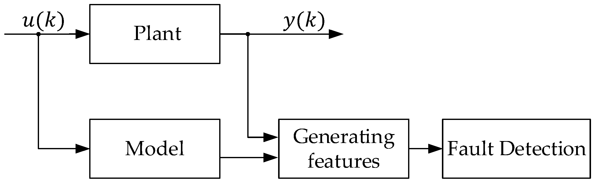
Figure 2.
Vector space of cross-correlation functions.
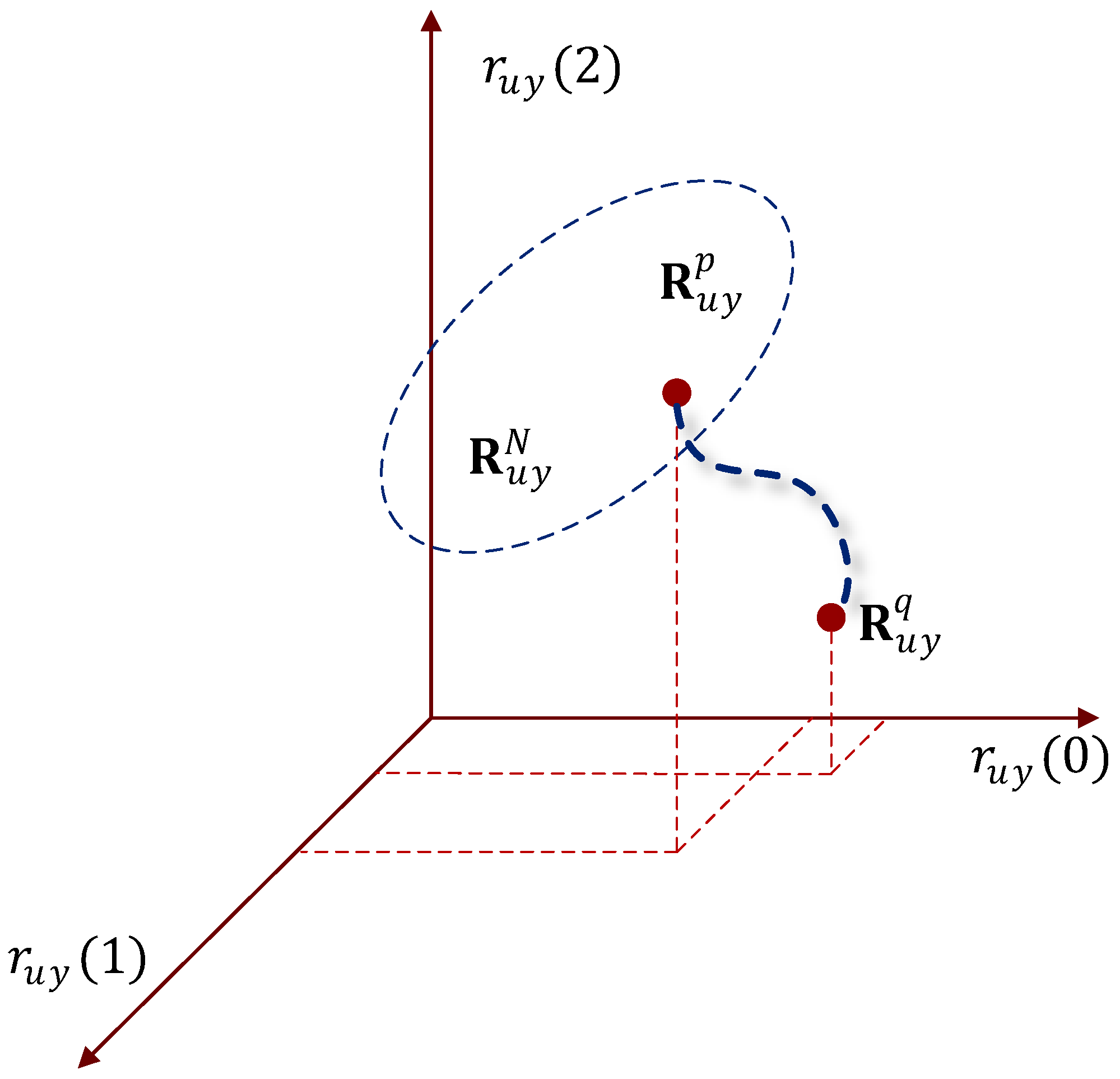
Figure 3.
Architecture of the neural network autoencoder.
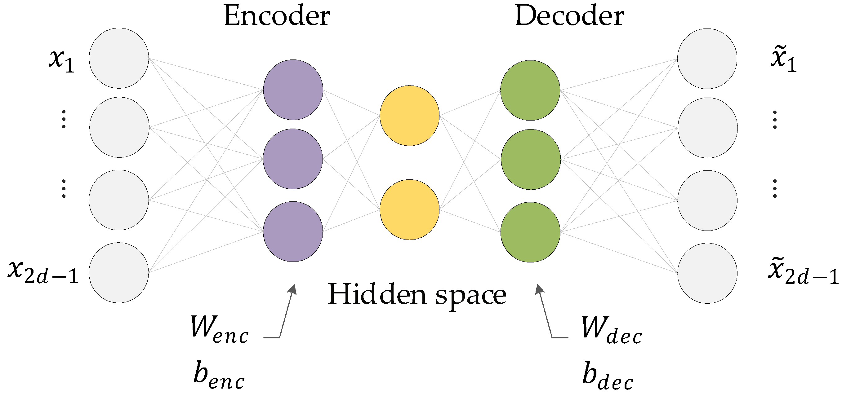
Figure 4.
Scheme for the synthesis of discord detector.
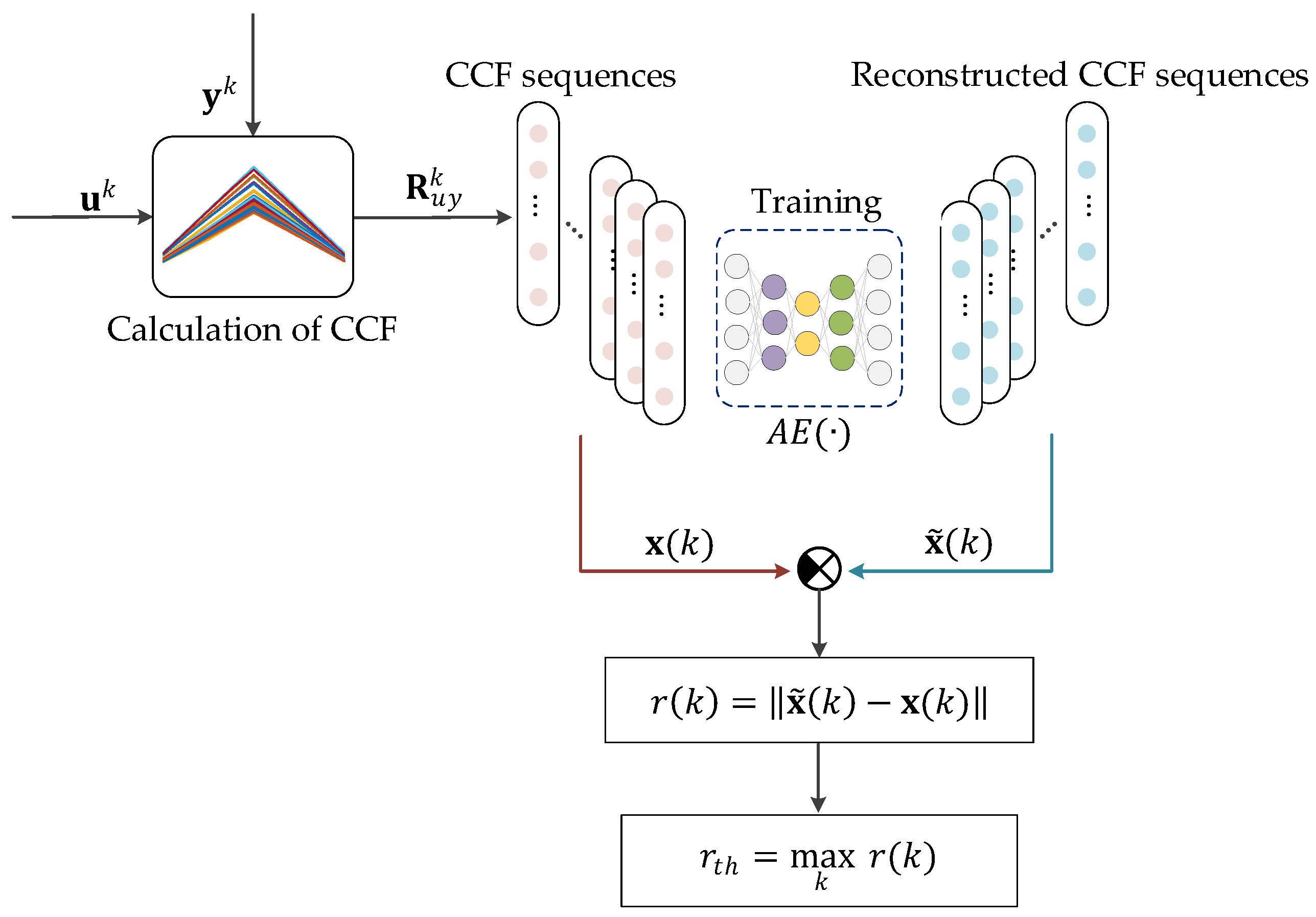
Figure 5.
Scheme for the application of disorder detector.
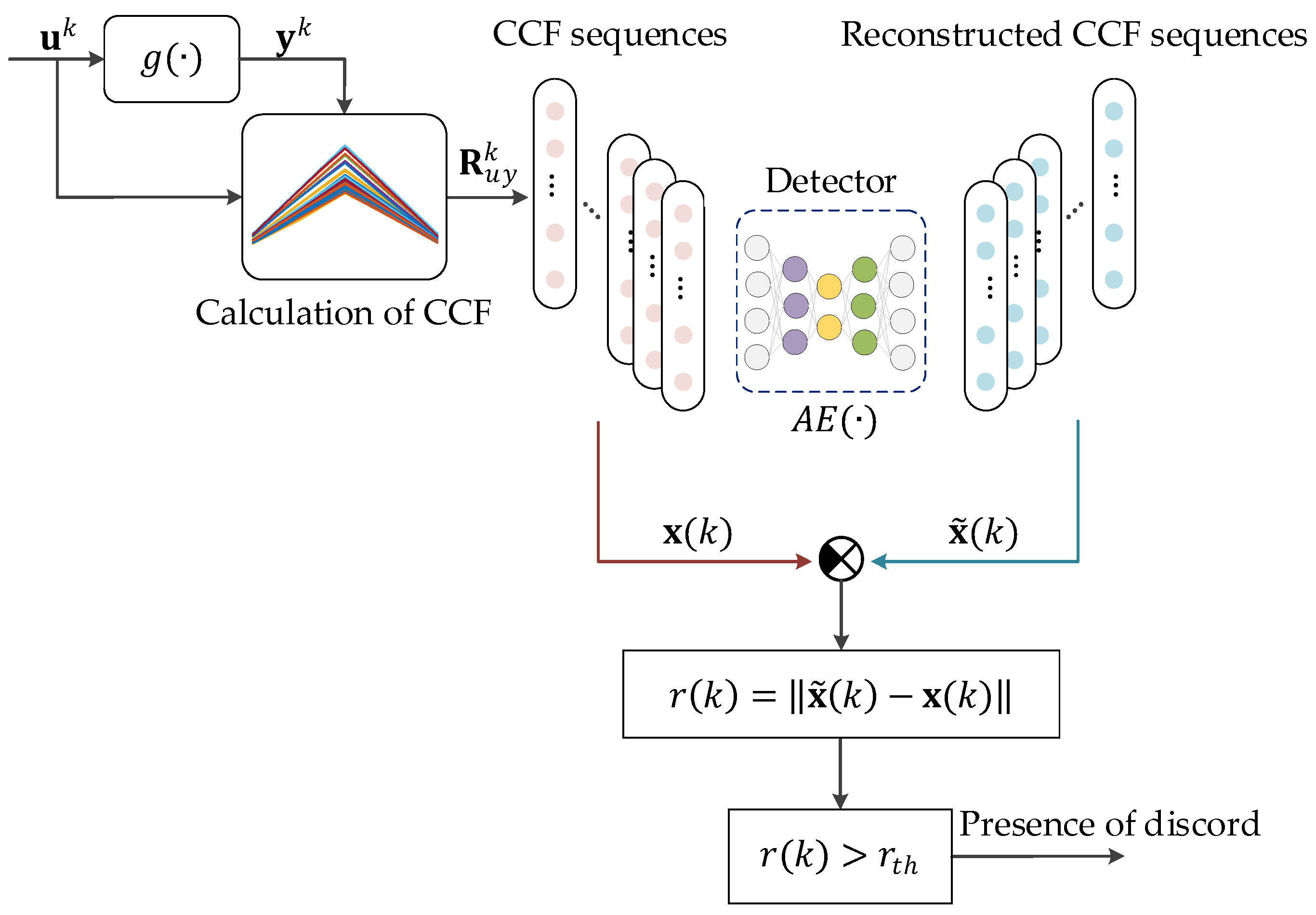
Figure 6.
Algorithm for detecting discord using CCF-AE (a) and algorithm for detecting discord using CUSUM (b).
Figure 6.
Algorithm for detecting discord using CCF-AE (a) and algorithm for detecting discord using CUSUM (b).
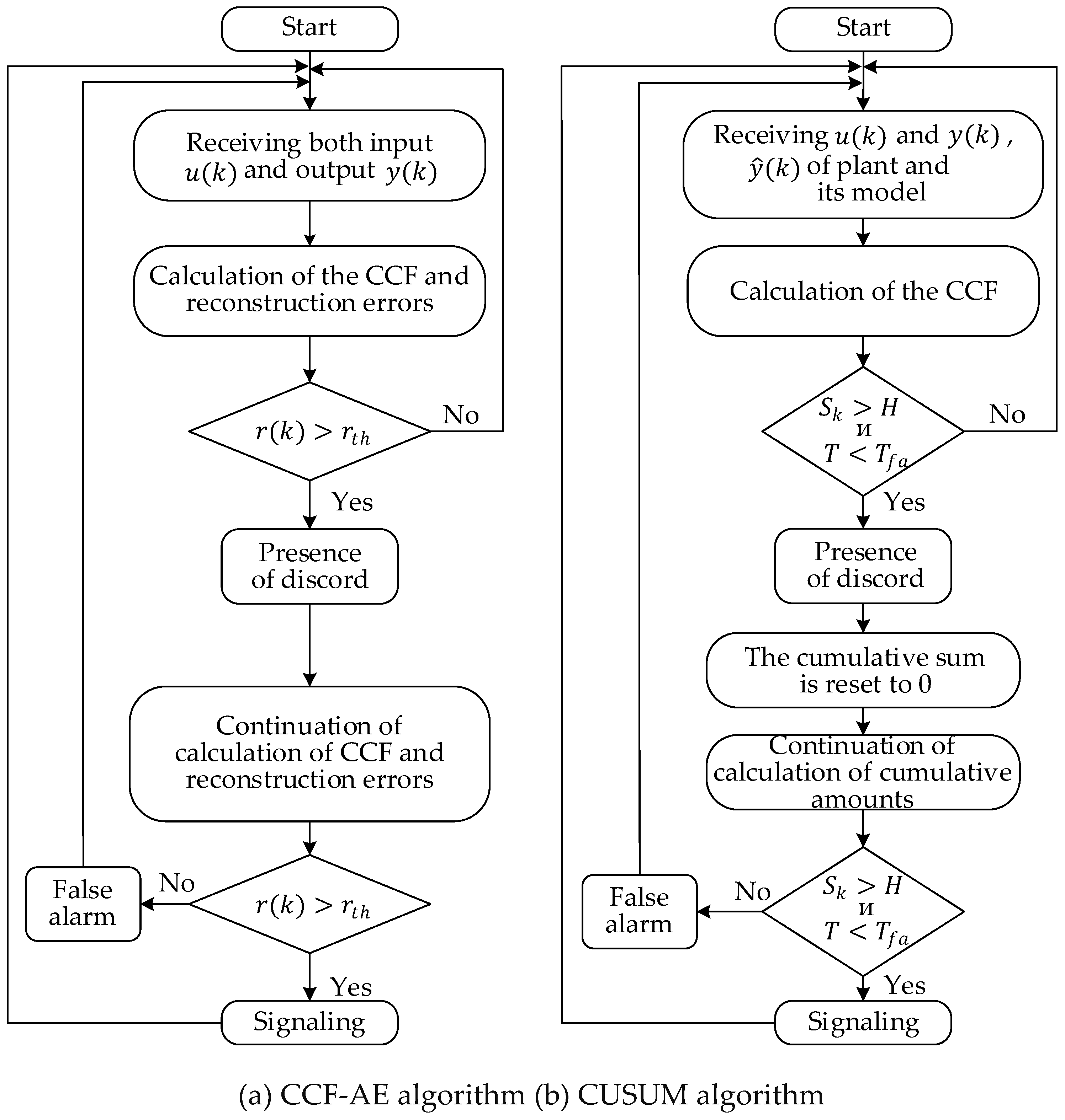
Figure 7.
The process of pH neutralization reaction.
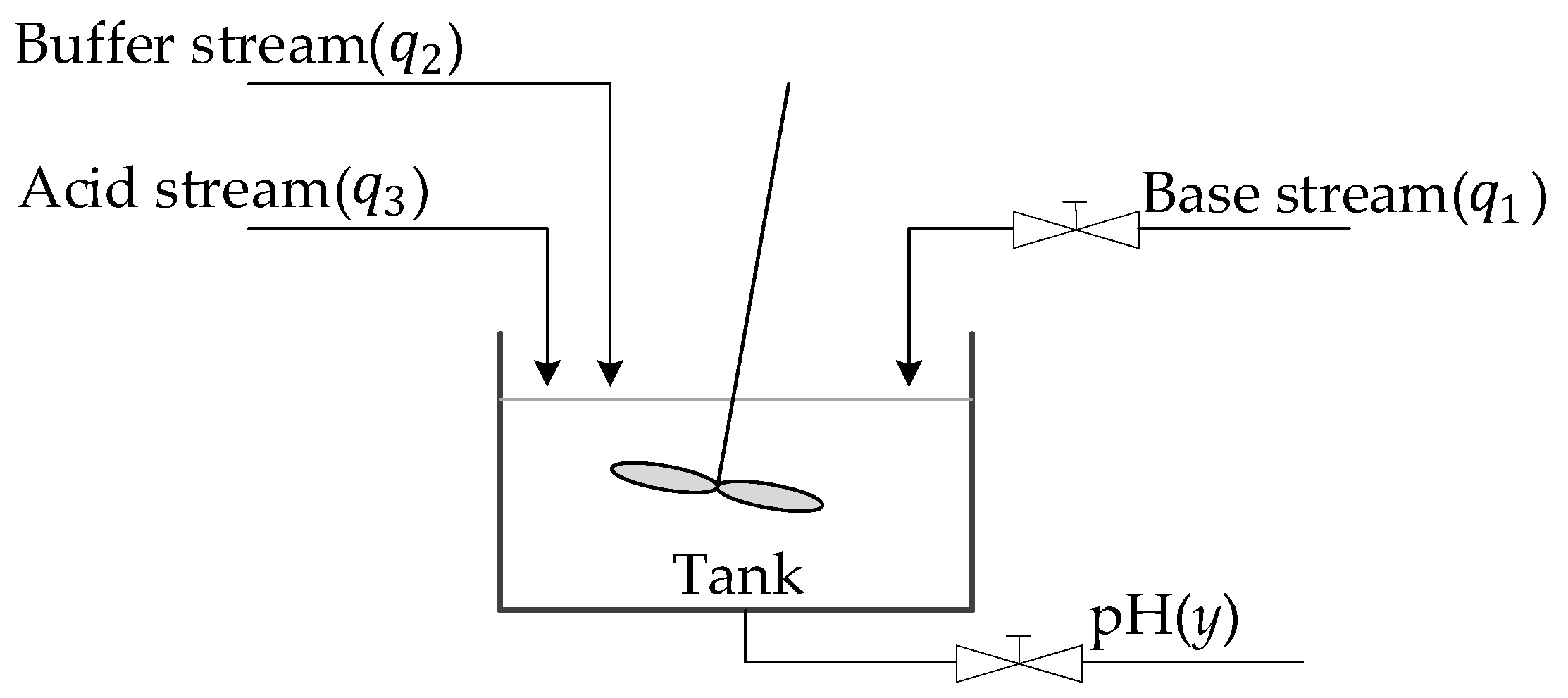
Figure 8.
Scheme for the neutralization reactor model in the SimInTech modeling package.
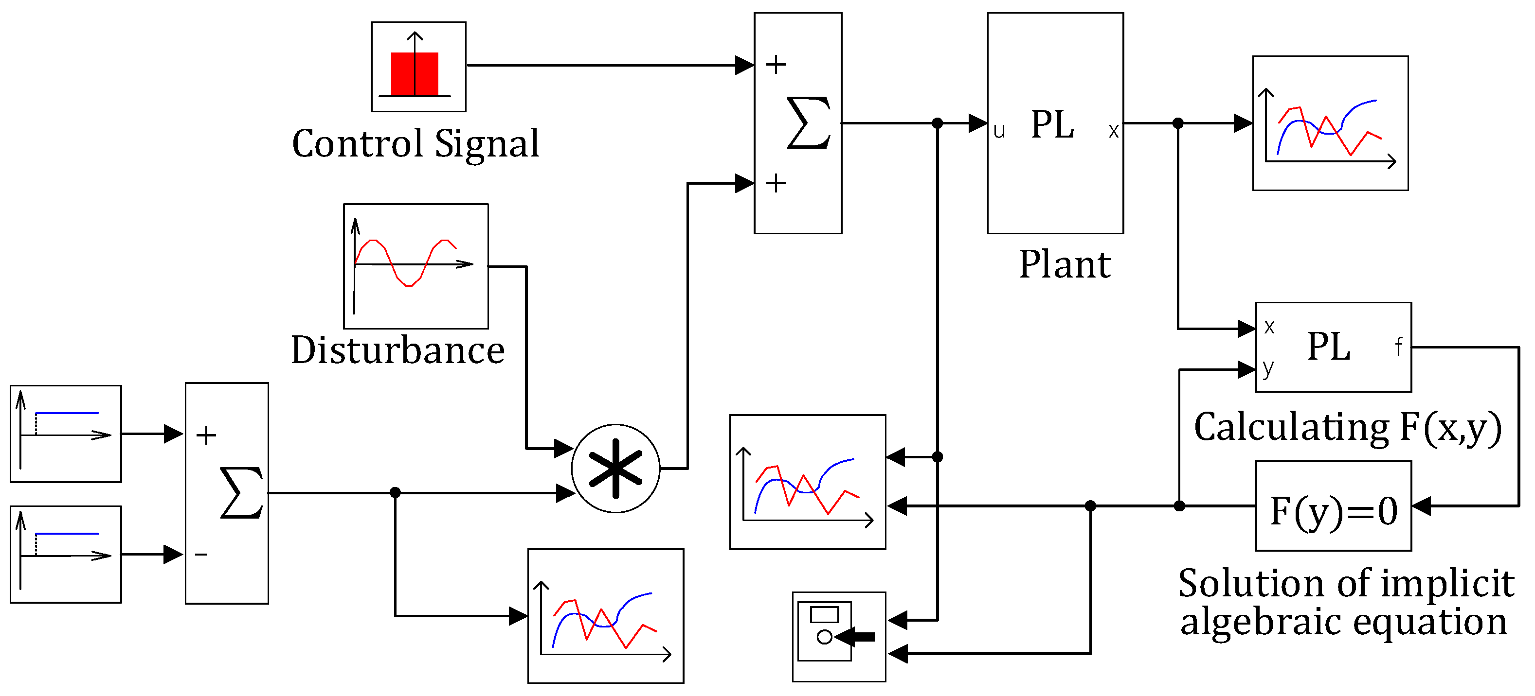
Figure 9.
Results of the neutralization reactor simulation.
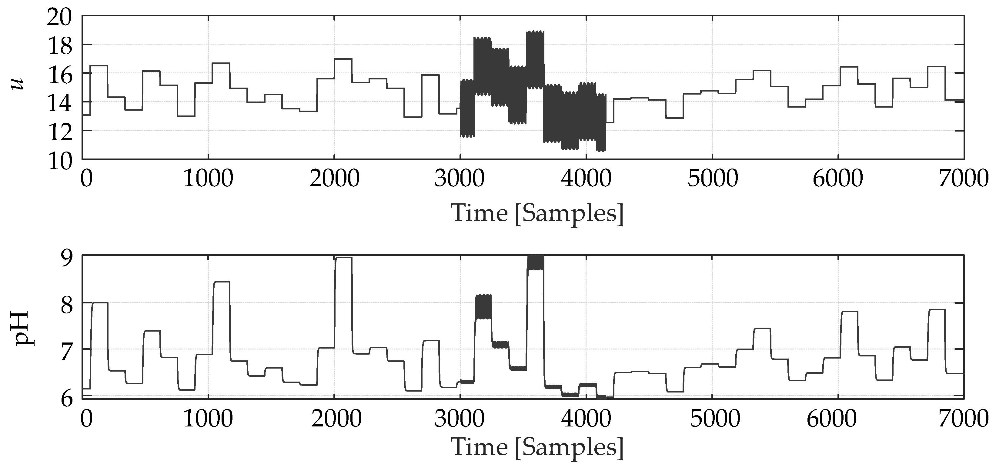
Figure 10.
CCF calculation results under a moving window of length 5.
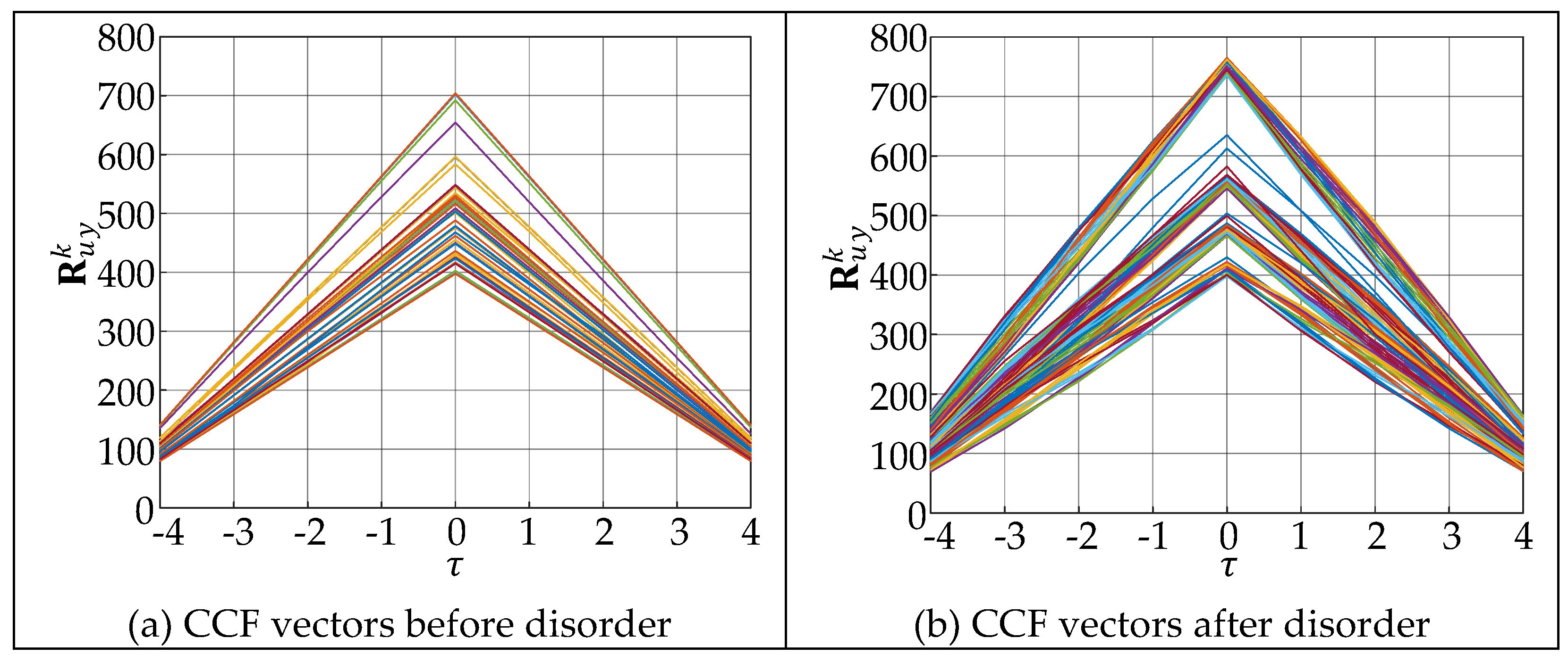
Figure 11.
Disorder detection results using the CCF-AE algorithm.
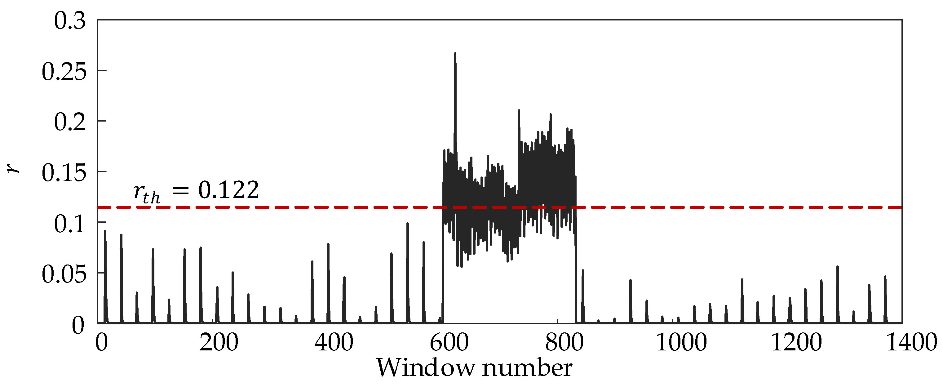
Figure 12.
pH values output by the GRU neural network model and the mathematical model on the SimInTech.
Figure 12.
pH values output by the GRU neural network model and the mathematical model on the SimInTech.
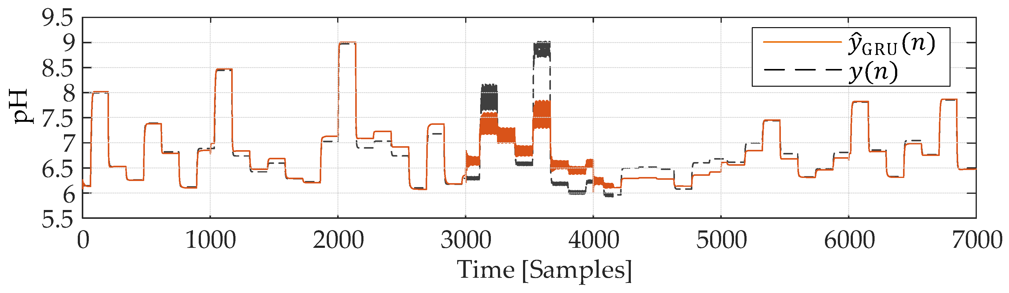
Figure 13.
Identification error of GRU neural network.
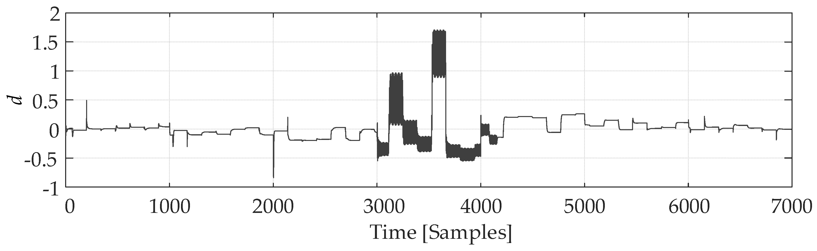
Figure 14.
Disorder detection results using the CUSUM algorithm.
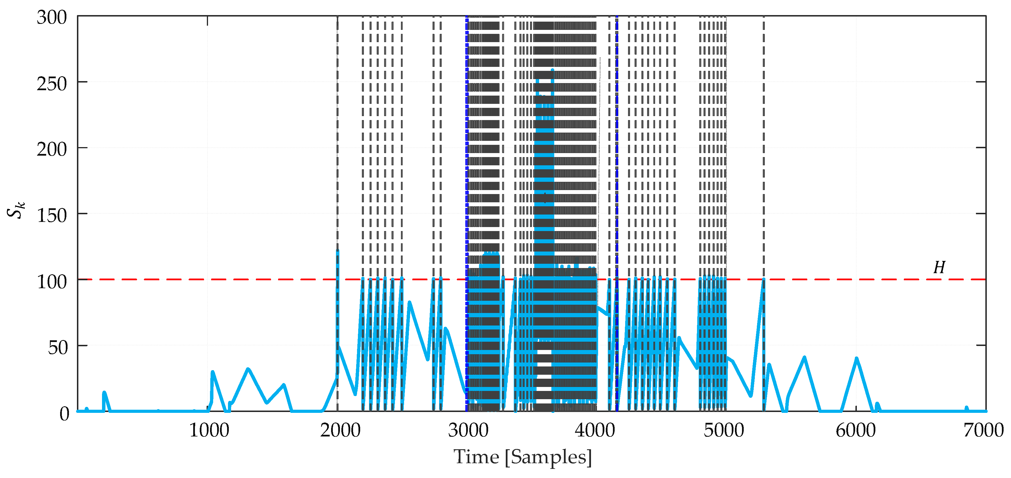

Table 1.
Parameters of the basic model of the neutralization reactor.
| Parameter | Value |
|---|---|
Table 2.
Nominal operating points of the neutralization reactor.
| Parameter | Value |
|---|---|
Table 3.
Results of discord detection by CCF-AE algorithm and CUSUM algorithm.
| Algorithm | ||
| CCF-AE | 0 | 5 |
| CUSUM | 89.11 | 5.42 |
Disclaimer/Publisher’s Note: The statements, opinions and data contained in all publications are solely those of the individual author(s) and contributor(s) and not of MDPI and/or the editor(s). MDPI and/or the editor(s) disclaim responsibility for any injury to people or property resulting from any ideas, methods, instructions or products referred to in the content. |
© 2024 by the authors. Licensee MDPI, Basel, Switzerland. This article is an open access article distributed under the terms and conditions of the Creative Commons Attribution (CC BY) license (http://creativecommons.org/licenses/by/4.0/).
Copyright: This open access article is published under a Creative Commons CC BY 4.0 license, which permit the free download, distribution, and reuse, provided that the author and preprint are cited in any reuse.


