Preprint
Article

This version is not peer-reviewed.

A Portable UV-LED/RGB Sensor for Real-Time Bacteriological Water Quality Monitoring Using ML-Based MPN Estimation

Submitted:

25 December 2024

Posted:

26 December 2024

You are already at the latest version

Abstract

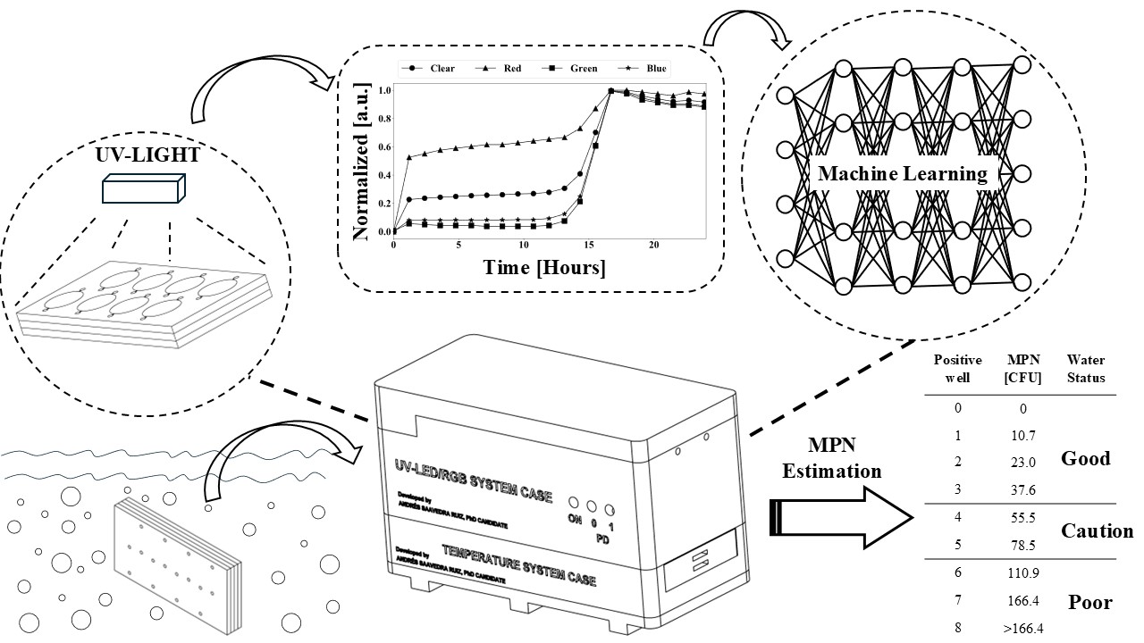
Bacteriological water quality monitoring is of utmost importance for safeguarding public health against waterborne diseases. Traditional methods such as Membrane Filtration (MF), Multiple Tube Fermentation (MTF), and enzyme-based assays are effective in detecting fecal contamination indicators, but their time-consuming nature and reliance on specialized equipment and personnel pose significant limitations. This paper introduces a novel, portable, and cost-effective UV-LED/RGB water quality sensor that overcomes these challenges. The system is composed of a microfluidic device for sample-preparation-free analysis, RGB sensors for data acquisition, UV-LEDs for excitation, and a portable incubation system. Commercially available defined substrate technology, Most Probable Number (MPN) analysis, and artificial intelligence are combined for the real-time monitoring of bacteria colony-forming units (CFU) in a water sample. By eliminating the need for sample preparation, specialized equipment, and laboratory space, the system provides an efficient and affordable solution for water quality monitoring in remote and resource-limited areas. The main significance lies in the combination of miniaturization, automation, and machine learning (ML) based data analysis. Multilayer perceptron neural networks (MLPNN) and support vector machine (SVM) are used to rapidly (30 minutes) predict RGB signals from water samples in wells. By predicting the number of positive wells, the system can predict the MPN of CFU in a water sample, allowing for the rapid estimation of bacterial concentration in a low-cost and portable manner.

Keywords: 
;  ;  ;  ;  ;  ;  ;  
Subject: 
Engineering  -   Bioengineering

1. Introduction

Waterborne diseases pose a significant threat to public health, leading to an annual occurrence of 7.15 million cases and 6,630 deaths in the United States alone [1]. This includes diseases such as cholera, typhoid fever, hepatitis, gastrointestinal ailments, and respiratory tract infections often originating from pathogenic microorganisms such as bacteria, viruses, fungi, and intestinal worms. As a result, monitoring water quality is indispensable for safeguarding public health and preserving ecological equilibrium [2,3].
Effective water quality analysis depends on measuring various parameters. While traditional physic-chemical indicators like potential of hydrogen (pH), electrical conductivity (EC), Turbidity (Turb), total dissolved solids (TDS), total phosphorus (TP), Total Nitrogen (TN), and dissolved oxygen (DO) offer insights into water quality [4], they don't directly reflect potential health or agricultural implications. The detection of bacteria, including total coliforms, Escherichia coli (E. coli), and Enterococcus faecalis (E. faecalis), is one of the most used metrics for assessing bacteriological contamination [5]. These indicators, characterized by distinct biochemical traits, serve as reliable markers to determine the suitability of water and food for human consumption [6]. The geometric mean (GM) and statistical threshold value (STV), measured in Colony-Forming Units (CFU) per 100 ml, are the statistical values used in bacteriological water quality standards. The 2012 Recreational Water Quality Criteria (2012 RWQC) recommends thresholds of 35 CFU per 100 ml GM for marine and freshwater enterococci and 126 CFU per 100 ml GM for E. coli in freshwater [7]. Similarly, the Beach Action Value (BAV) defines limits of 70 CFU per 100 ml for marine and freshwater enterococci and 235 CFU per 100 ml for E. coli in freshwater [7].
Established methods such as multitube fermentation (MTF) and membrane filtration (MF) are often viewed as the gold-standard for assessing water quality. These techniques are supported by standardized and accredited protocols that facilitate inter-laboratory comparisons. However, they present drawbacks including the need for cold transportation, trained personnel, laboratory space and equipment, expensive consumables, and a minimum 24-hour incubation period for obtaining results. Alternative methods include molecular and enzyme-based techniques, which mitigate some of these drawbacks and offer significantly faster detection [8,9]. The defined substrate technology (DST) method, exemplified by ColilertTM and EnterolertTM (IDEXX Laboratories, Inc., Maine, USA), uses enzyme-substrate fluorescence to quantify total coliforms, E. coli, and enterococci [10,11]. This EPA-approved approach is easier to use than traditional methods and features a streamlined process, although it may involve human error during quantification. The IDEXX Quanti-Tray system divides a 100 mL sample into 51 wells and uses the most probable number (MPN) method to determine the bacterial count in the original sample [11]. However, like MTF and MF, DST requires specialized laboratory equipment, cold transportation, and has an incubation time of 24 hours per test.
Recent advancements in sensor technology have introduced alternative methods to accelerate bacterial detection. For instance, the Colifast ALARMTM, developed by the Norwegian company Colifast (Colifast AS, Lysaker, Norway), automates detection and reduces the time to detection by using DST and focusing on the presence of fluorescence due to bacterial growth. The system collects and incubates water samples in a specialized chamber connected to a detector. The substrate 4-methylumbelliferyl-β-D-glucuronide is used for detecting E. coli, while 4-methylumbelliferyl-β-D-galactoside is used for detecting total coliforms [12,13]. However, a disadvantage of this system is that it requires installation in a fixed setting, limiting its use in field applications and potentially increasing the operational costs due to the need for dedicated space and technical oversight. Additionally, the company has developed the Colifast Field Kit, which enables measurements within 75 minutes to 2 hours and is more cost-effective than the standard version. However, its detection limits are tailored to concentrations above 500 CFU per 100 mL. However convenient, many of these systems require investments between thousands to tens of thousands of dollars.
Microfluidic devices can offer solutions to some of these limitations due to their low-cost, portability, potential for automation, and ability to capture and analyze small volumes. As a result, lab-on-a-chip sensors have been developed for water quality monitoring, specifically for detecting microorganisms, heavy metals, organic compounds, and various other substances [14]. Recent research has led to the development of microfluidic-based technologies that enable the monitoring of multiple water contaminants with precision comparable to traditional methods, while significantly reducing detection times. In one such study, Gowda et al. designed a microfluidic device capable of capturing water samples, lysing bacterial cells, extracting nucleic acids, and quantifying bacteria using a droplet digital loop-mediated isothermal amplification assay. This portable system can quickly detect bacteria like E. faecalis directly on-site, completing the entire test in just 1 hour and requiring less than 5 minutes of manual sample handling [15].
Additional innovations aimed at reducing the detection time for E. faecalis have included recombinase polymerase amplification (RPA) combined with a lateral flow assay (LFA). This method allows for testing within approximately 30 minutes, a significant reduction compared to the 24 hours required by the Enterolert™ test. However, the RPA-LFA approach compromises sensitivity, detecting E. faecalis with 10 to 1000 times lower efficiency compared to Enterolert™ [16]. This highlights the ongoing challenge of developing low-cost technologies that are both rapid and sensitive enough for effective water quality monitoring.
To accelerate the detection of bacteria in water, machine learning (ML) can be used with lab-on-a-chip concepts to efficiently capture, monitor, and store water samples. As a branch of artificial intelligence (AI), ML involves creating algorithms that enable computers to learn from data and enhance their performance over time [17,18]. By developing mathematical models that identify patterns and relationships within datasets, ML can predict the behavior of new data, making it an effective tool for real-time water quality monitoring. Paepae et al. examined the most used parameters and machine learning (ML) algorithms in water quality research. They identified four predominant algorithms: Neural Networks (NN), Random Forest (RF), Multiple Linear Regression (MLR), and Support Vector Machines (SVM) [4]. Neural Networks were favored for their ability to model complex nonlinear relationships in water quality data, making them highly suitable for tasks requiring high predictive accuracy [19]. Random Forest gained popularity for its robustness, capacity to handle large datasets with high dimensionality, and effectiveness in reducing overfitting [20,21]. The multiple linear regression (MLR) facilitates hypothesis testing and model selection. To enhance reliability and consistency, steps such as multicollinearity diagnostics, cross-validation, and regularization are conducted prior to model development. In water quality index (WQI) modeling, MLR integrates multiple physicochemical parameters into a single score that represents overall water quality [22]. The Support Vector Machine (SVM) algorithm works well with small datasets but can face computational efficiency issues with larger ones. Conversely, limited sample sizes may not sufficiently capture classification features. Effective data streamlining is essential to preserve support vectors and maintain data integrity [23].
In this study, rapid prototyping and open-source tools are used to create a water quality sensor having a microfluidic device and everything necessary to carry out and quantify a DST assay at the point-of-care. MPN quantification occurs by observing the number of positive (fluorescing) wells in the microfluidic device. Each well is loaded with the Enterolert™ substrate mixed with bacteria-containing water and placed within a portable incubation system. The system uses UV light excitation and RGB sensors to monitor the water samples in each well, generating a dataset to train two machine learning algorithms: Multilayer Perceptron Neural Networks (MLPNN) and Support Vector Machine (SVM). Once trained, the ML can quickly predict whether a well will be positive or negative after the 24-hour period. In conjunction with the MPN table, this technique predicts the water sample MPN in a few hours, using low-cost, open-source materials.

2. Materials and Methods

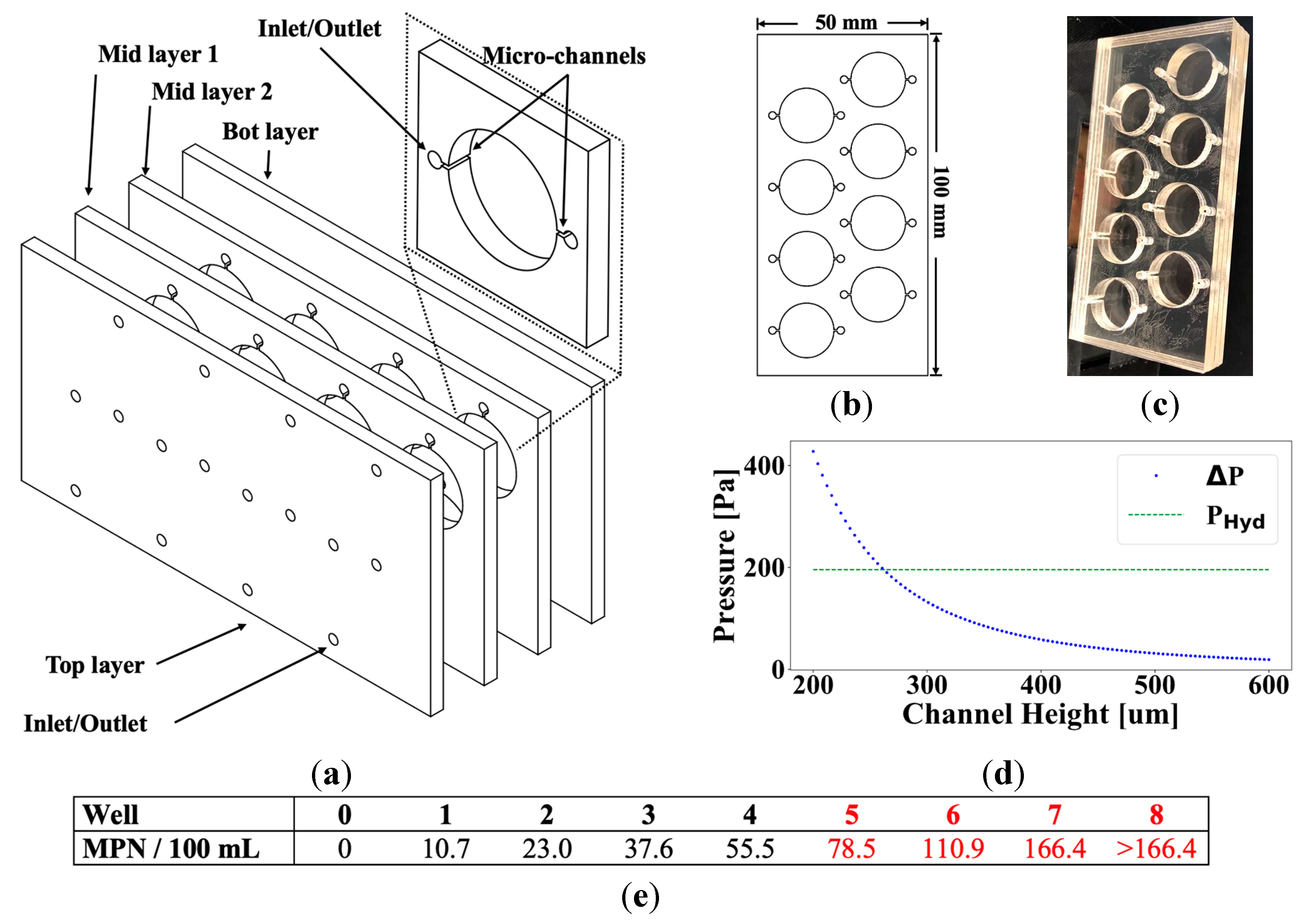
2.1. Microfluidic Device Design & Loading

The microfluidic device was designed to facilitate both sample handling and Most Probable Number (MPN) quantification of bacteria. The microfluidic device was constructed from four acrylic sheets including a base sheet without apertures, two intermediate sheets, each featuring eight wells with channels for fluid movement, and a top sheet solely for fluid inlets/outlets, Figure 1a. The dimensions of each acrylic sheet measured 50 mm x 100 mm, and the wells possessed a diameter of 16 mm, Figure 1b. Inlet and outlet ports connect to each well through channels of 500 µm height, h, 3.175 mm width, w, and 22 mm length, L, respectively; L was taken as the distance between inlet and outlet ports. The fabrication of the device used 3.175 mm cast acrylic sheets and an Epilog 60W CO2 laser cutter, Figure 1c. The microfluidic device was designed to fill with liquid passively by comparing the approximate hydraulic resistance of the channels ( R H y d = ( 12 μ L ) / ( 1 0.63 h w h 3 w ) to the hydrostatic pressure ( P H y d = ρ g L ) provided at the channel inlet when submerged. A comparison is shown in Figure 1d where Phyd represents the pressure necessary to overcome the hydraulic resistance of the channel and ∆P is the hydrostatic inlet pressure ( P = Q R H y d ) , assuming a volumetric flow rate Q of 5 mL/min. The analysis demonstrated that for the selected dimensions (L = 22 mm, w = 3.175 mm), a channel height h above 280 μm results in efficient filling, while heights below led to incomplete filling due to a lack of inlet pressure. Figure 1e displays the MPN table for the microfluidic device using equation 1, obtained from Jarvis et. al. [24], where t p refers to the number of positive tubes, t T is the total number of tubes, d e t is the dilution level per tube, and v e t is volume per tube. Additionally, equation (2) was used to calculate the confidence limits ( C I l i m i t ), where σ represents the standard deviation associated with each MPN value, d.
M P N = L n 1 t p t T ( d e t ) v e t
C I l i m i t = d e 2 σ ln d , d e 2 σ l n ( d )
The volume and number of wells was chosen to include the EPA BAV threshold of 70 CFU, which is the limit used to determine if water is suitable for recreational activities. The detection range, when all wells are positive, is 166.4 CFU/100mL. The detection range and resolution could be tailored for different applications and involves changing the number of wells and volume per well.
Experiments used 108 mL of distilled water and a lyophilized E. faecalis pellet (Enterococcus faecalis WDCM Vitroids™, Sigma-Aldrich Co. LLC, St. Louis, Missouri) hydrated in 2 mL of PBS. The IDEXX Enterolert™ reagent is then added to the 110 mL solution and is thoroughly shaken to ensure homogeneity. The microfluidic device is filled with 10 mL of this mix, while 100 mL is used to fill the IDEXX Quanti-Tray/2000. The inlets and outlets of the microfluidic device are sealed with Polyester Film PET tape and incubated for 24 hours in a portable platform. The Quanti-Tray is incubated for 24 hours in an incubator oven at 41 °C.

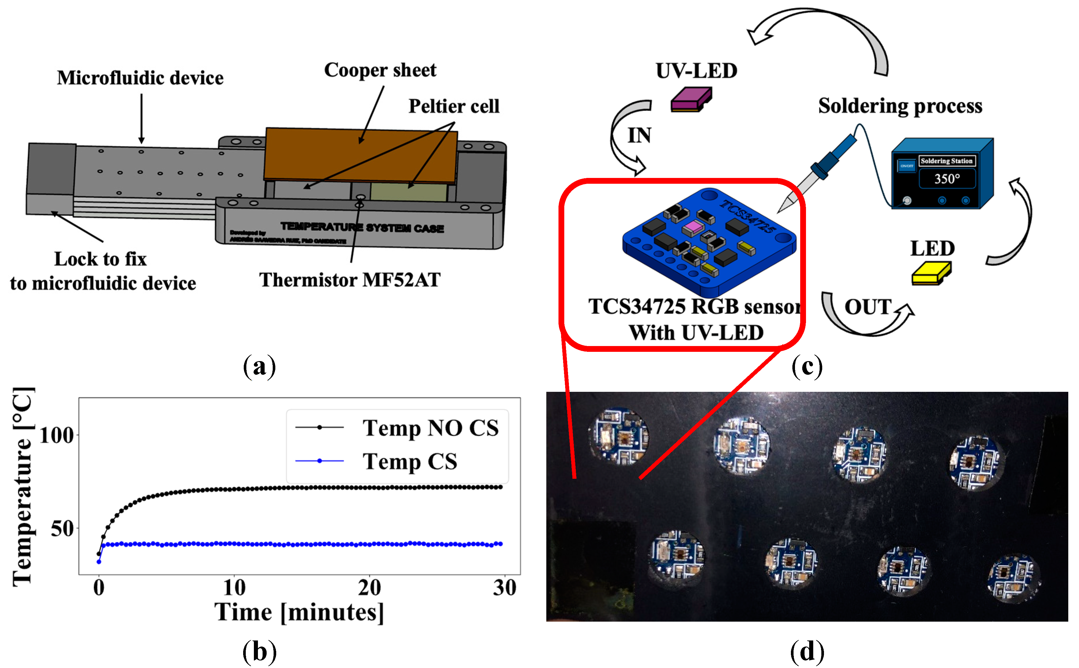
2.2. Portable Temperature-Controlled Incubation and UV-LED/RGB Excitation & Emission System for Bacterial Detection

Achieving the required incubation temperature of 41°C for a 24-hour period is vital for accurate results. A temperature control system was developed using a Peltier thermoelectric cooler (Digi-key Electronics, TEC-12706, MN 56701 USA) as the heating element, a copper sheet to distribute heat, and a thermistor (Einstronic, MF52AT, Sabah, Malaysia) as the temperature sensor. These components are controlled by an Arduino Nano 33 IoT (Digi-key Electronics, part ABX00027, MN 56701 USA), which interfaces with the Peltier cell via a motor drive module (Einstronic, MX1508, Sabah, Malaysia). A customized case was designed in Solid Works and fabricated using a 3D printer (Creality CR 10S, Shenzhen, China) and holds the Peltier cell, copper sheet, and microfluidic device, Figure 2a. Figure 2b presents the temperature response of the system with and without a control system (CS), demonstrating the effectiveness of the control system in stabilizing temperature fluctuations.
The UV-LED/RGB system combines RGB sensors (Adafruit Industries LLC, TCS34725, New York USA) with UV LEDs (Digi-key Electronics, part 1497-1479-1-ND, MN 56701 USA), all controlled by the Arduino Nano 33 IoT. Originally designed with an LED emitter, the RGB sensors are calibrated using various color sheets (White, Black, Red, Green, and Blue). UV LEDs are then integrated into the RGB sensor system to enable fluorescence detection in water samples, Figure 2c. To enhance accuracy and minimize noise, a black acrylic layer is incorporated into the RGB system as a filter, effectively reducing UV light scattering, Figure 2d.
The UV-LED/RGB system is designed with a temperature control unit at the base, where the microfluidic device is inserted. The RGB sensor monitoring system is positioned in the upper section, Figure 3a. These RGB sensors communicate with the microcontroller using I2C communication protocol, with a multiplexer (Texas Instruments, TCA9548A, Texas, USA) enabling simultaneous communication with up to eight RGB sensors. Data can be viewed in real time through either wired or wireless connections. A comprehensive database is constructed, incorporating clear, red, green, and blue signals for each sensor, yielding a total of thirty-two columns of data.
Figure 3b shows a summary of results from an experiment using a water sample inoculated with a 50-80 CFU pellet. The IDEXX Quanti-Tray/2000 was used as a benchmark and measured a bacterial concentration of 35 CFU/100mL while the UV-LED/RGB system measured 37.6 CFU/100mL, using the same water sample and the custom-made MPN table, Figure 1e. Figure 3c shows red, green, blue, and clear (RGBC) channel data for individual wells in the microfluidic device. It is important to note that bacterial quantification can be performed by counting the number of positive wells after 24 hours, but this time-to-detection can be greatly reduced by studying the RGBC curves in real-time during incubation. Data was acquired every 20 seconds resulting in 4320 observations in a 24-hour incubation period. Figure 3d shows a picture of the microfluidic device when exposed to UV light. The device's wells are numbered from 0 to 7. Fluorescence appears in wells 4, 6, and 7, indicating a CFU of 37.6 CFU according to Figure 1e. This fluorescence corresponds to the exponential growth curves in Figure 3c at approximately hour 15 for wells 4, 6, and 7, and serves to confirm the growth detected by the UV-LED/RGB system.

2.3. Machine Learning (ML) Algorithms

Two machine learning (ML) algorithms, Support Vector Machine (SVM) and Multilayer Perceptron Neural Networks (MLPNN), were selected for this study due to their widespread application in water quality analysis.
Equation 3 applies the first derivative to the RGB sensor signals, denoted as "c" for Clear, "r" for Red, "g" for Green, and "b" for Blue. This transformation is incorporated into the dataset used by machine learning algorithms to enhance their performance.
c ( t ) d t ,   r ( t ) d t ,   g ( t ) d t ,   b ( t ) d t
The SVM algorithm was developed in Python, an open-source software, using a combination of ML and data manipulation libraries such as NumPy, Pandas, Scikit-Learn, TensorFlow, and Keras. A normalized and derivative-transformed dataset (using Equation 3) includes measurements from 8 UV-LED/RGB sensors, with inputs for each sensor representing values for clear, red, green, and blue, both in their original and derived forms. The dataset is divided into training and testing sets with a 70:30 ratio using Scikit-Learn's train_test_split function. The SVM model is fitted with a polynomial kernel, with tuned parameters (C=100, gamma='scale', coef0=0.5, degree=4), to capture non-linear relationships in the data. The model's performance is evaluated using metrics such as accuracy, precision, recall, and F1-score, represented by Equations 4 through 7 [25], where TP stands for true positives, TN for true negatives, FP for false positives, and FN for false negatives. These metrics are visualized for each sensor using bar graphs, and the results are plotted using Matplotlib to generate detailed graphs of each sensor's performance.
Similarly, the MLPNN algorithm was implemented in Python, leveraging TensorFlow and Keras for building and training the neural network model. The data preprocessing steps involved loading normalized and derivative-transformed datasets, followed by splitting the data into training and testing sets. The neural network architecture consisted of a sequential model with multiple dense layers, configured with 32 neurons in each hidden layer (2) and using the 'tanh' activation function to capture complex relationships between input features. The model was optimized using the 'adam' solver and an adaptive learning rate, with regularization parameter alpha set to 0.001, and the maximum number of iterations increased to 1000 to ensure convergence. As with SVM, the performance of the MLPNN model was evaluated using metrics such as accuracy, precision, recall, and F1-score (equations 4 – 7, respectively) [25], which are visualized for each sensor using bar graphs, ensuring robust model development. A plotting stage was also included to visualize the predicted and actual values, demonstrating the model's ability to generalize across different datasets.
A c c u r a c y = T P + T N T P + T N + F P + F N
P r e c i s i o n = T P T P + F P
R e c a l l = T P T P + F N
F 1   S c o r e = 2 ( P r e c i s i o n ) ( R e c a l l ) P r e c i s i o n + R e c a l l

3. Results and Discussion

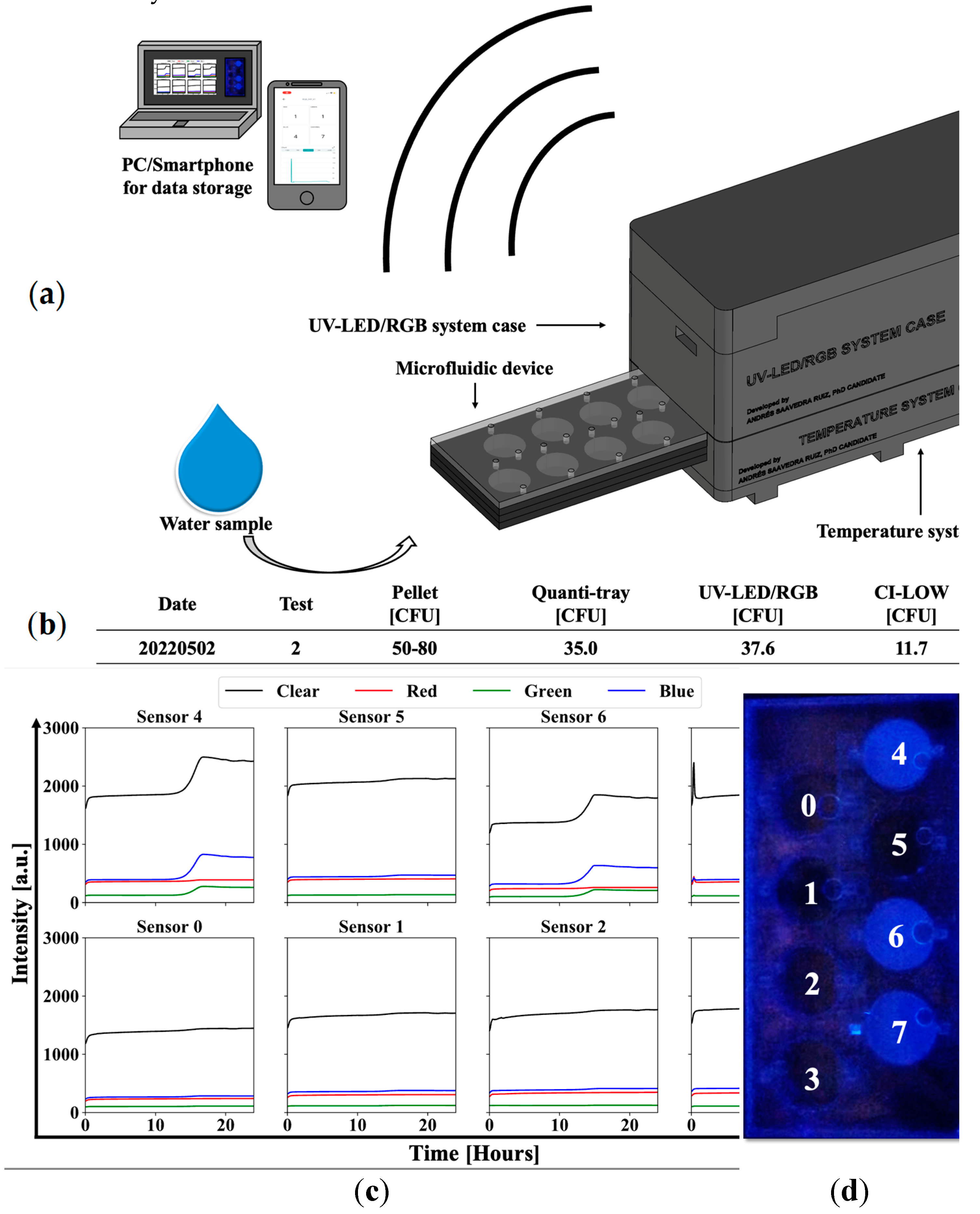
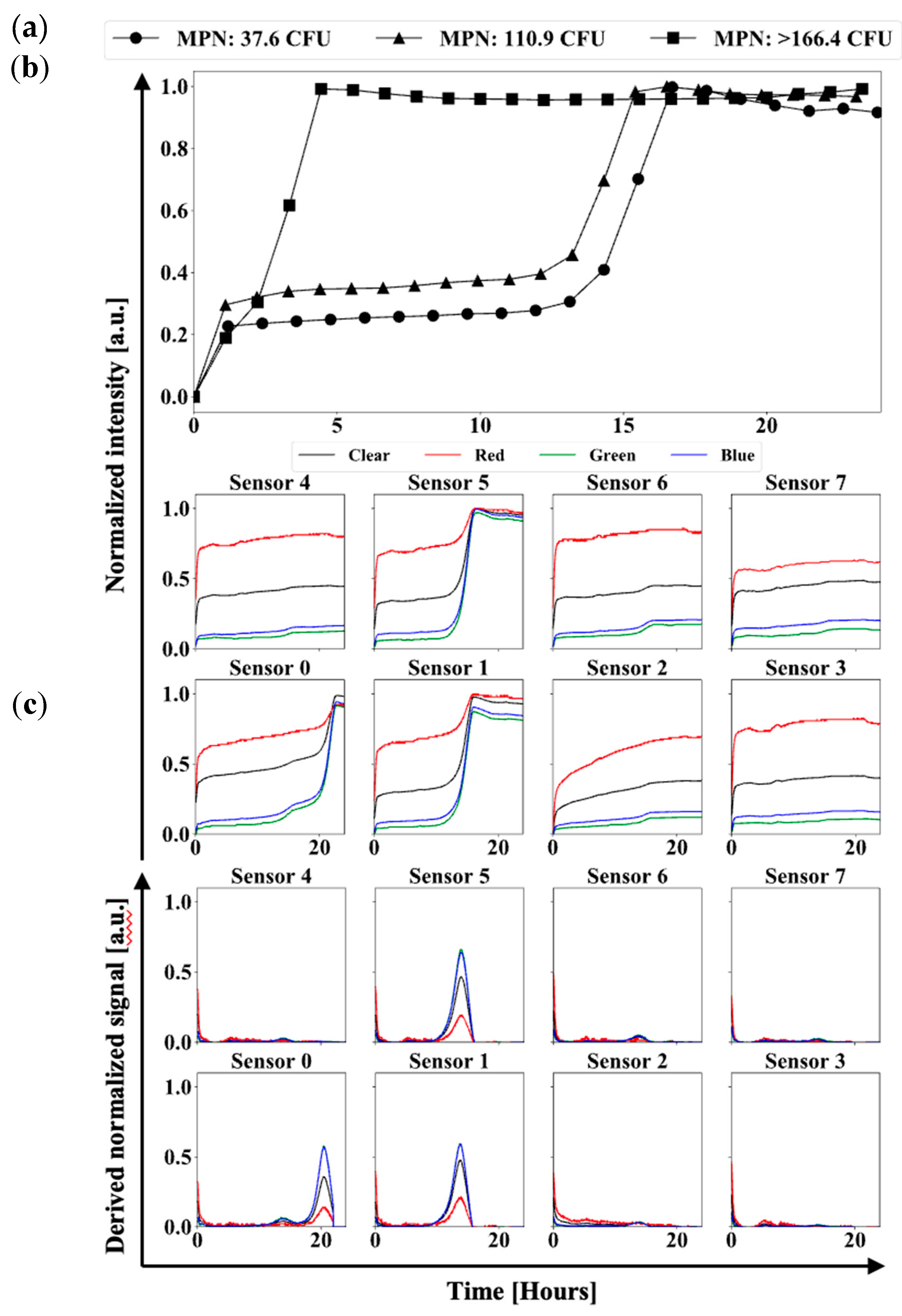
3.1. UV-LED/RGB System

Several experiments were conducted using the UV-LED/RGB system, comparing its results with those obtained from the IDEXX Quanti-Tray/2000 system. The experiments were carried out using different concentrations of bacteria to assess the performance of the UV-LED/RGB system. Figure 4a shows “clear” color channel signals from sensor number 4 for experiments having different bacterial concentrations; 37.6, 110.9, and >166.4 CFU/100mL. All curves exhibit the characteristic sigmoidal behavior of bacterial growth, confirming the system's ability to monitor bacterial growth in real time. It can be observed that as the bacterial concentration increases, the growth curve's slope becomes steeper, and the exponential phase begins earlier.
Figure 4b illustrates the normalized signals from an experiment with a bacterial concentration of 37.6 CFU. Wells 0, 1, and 5 demonstrated a positive response to the presence of bacteria, as indicated by their sigmoidal trends throughout the incubation period, unlike the other wells. This figure provides a clear example of monitoring low bacterial concentrations in water, adhering to the EPA BAV standards for recreational activities (37.6 CFU/100mL). The exponential phase for wells 1 and 5 occurs at approximately 12 hours into the incubation period, suggesting that this duration is necessary to detect bacterial presence. In contrast, well 0 required more than 20 hours to reach the exponential phase, highlighting that solely interpreting sensor signals might not be sufficient for accurately determining bacterial concentrations in water samples within the first 12 hours.
Figure 4c presents the first derivative of the normalized signals from the same experiment, highlighting the same wells, 0, 1, and 5, as positive. Applying the first derivative to the normalized data serves as an alternative method to determine contamination in wells. It also helps in reducing the detection time of bacterial growth in the wells because the positive slope of the exponential phase first derivative can easily be distinguished from the flat curves of non-fluorescing wells. The first derivative data also provides additional information to the ML algorithms for predicting wells with bacterial contamination.

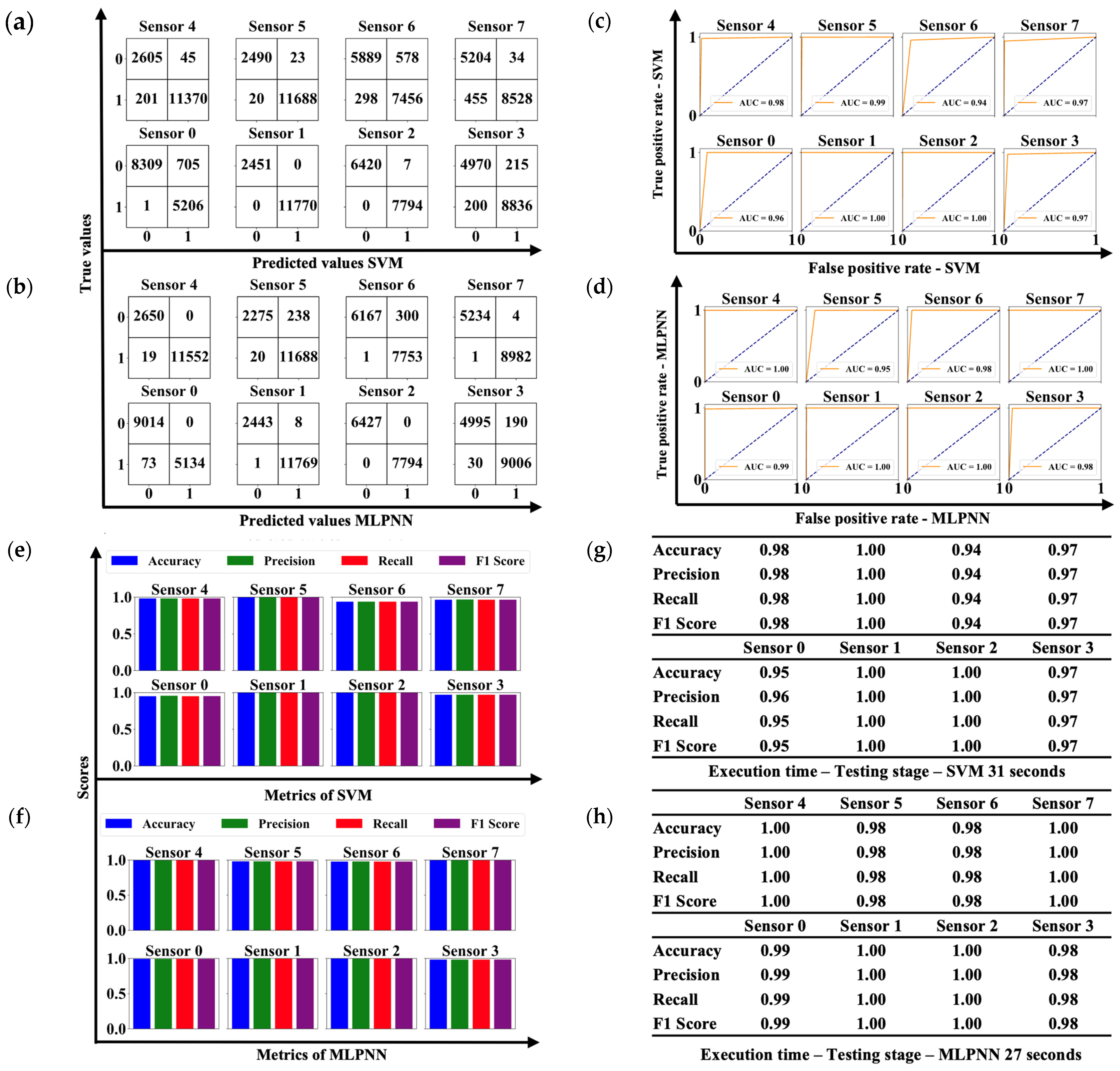
3.2. Machine Learning Algorithms

The database for the ML algorithms is divided into 70% for the training stage and 30% for the testing stage. During the training stage, the output variable, or target, is defined by assigning a "0" for the absence of bacteria in the well and a "1" for the presence of bacteria. Initially, the full 24 hours of data from each experiment is used to develop the model. Subsequently, the database is restricted to the lag phase in the experimental data, allowing the ML algorithms to analyze this phase with the aim of reducing the detection time.
Figure 5a,b illustrates the confusion matrix for each sensor when using the SVM and MLPNN algorithms, respectively, providing a visual representation of performance in terms of correct and incorrect classifications. The receiver operating characteristic (ROC) curves for both models are presented in Figure 5c,d, highlighting each algorithm's discriminative capability through their respective areas under the curve (AUC). The graphs comparing accuracy, precision, recall, and F1 score metrics between the algorithms are displayed in Figure 5e,f, emphasizing the performance differences between SVM and MLPNN. Figure 5g,h presents the metrics in tabular form alongside the execution times for each algorithm, offering a concise and comparative summary of their efficiency and effectiveness.
Upon analyzing Figure 5g,h, it becomes evident that the performance of the MLPNN and SVM algorithms was evaluated across several sensors, with both demonstrating high effectiveness in data classification, consistently achieving strong metrics in accuracy, precision, recall, and F1 score. However, the comparative analysis reveals subtle differences between the two models. MLPNN exhibited more consistent performance, achieving perfect or near-perfect metrics across most sensors, including sensors 4, 6, and 0, where it achieved exceptional results with values of 1.00 or 0.99 in all metrics. On the other hand, SVM also showed excellent performance, achieving perfect metrics in sensors 5, 1, and 2. Nevertheless, it experienced a slight decline in performance on other sensors, particularly on Sensor 6, where the metrics dropped to 0.94. Sensors 7 and 3 exhibited slightly lower metrics with the SVM algorithm, reaching values of 0.97. This variability suggests that while SVM is robust, it may face more challenges in correctly classifying in certain specific contexts or may require further fine-tuning of its hyperparameters or data preprocessing techniques to match MLPNN's consistency.
In terms of efficiency, MLPNN completed its execution in 27 seconds, while SVM took 31 seconds. Although both times were relatively quick, MLPNN was not only more consistent in its performance but also slightly more efficient in terms of execution time. These results suggest that MLPNN may better handle certain data patterns and offers more robust and efficient classification compared to SVM in this set of tests.
The UV-LED/RGB was shown to predict bacteria concentration in as little as half an hour by analyzing the lag phase of the sigmoidal curve. It was previously shown that the system quantifies bacteria concentration using the MPN method and counting how many wells are positive at the end of the 24-hour incubation period. Predicting the bacteria concentration was performed by using trained MLPNN and SVM algorithms that predicted which individual wells would be positive in 24-hours using only data from the lag phase. Table 1 shows the performance of each algorithm using data from different periods of the lag phase (3, 2, 1, and 0.5 hours) and highlights the performance of MLPNN and SVM for concentration prediction.
While MLPNN excelled with nearly perfect metrics in sensors 0, 1, and 2 during longer latency phases (3 hours), its performance declined notably as the latency period shortened, particularly in sensors 3, 6, and 7, where accuracy dropped as low as 0.72 at 0.5 hours. This suggests that MLPNN struggles to maintain consistency in scenarios requiring faster response times, likely due to the complexity of the temporal data patterns. In contrast, SVM demonstrated greater robustness across all latency phases, achieving consistently high accuracy even in shorter latency windows. For example, while MLPNN saw a marked reduction in performance at 0.5 hours, SVM maintained relatively stable metrics, only showing slight drops in sensors 2, 3 and 5. This resilience in SVM suggests that, although slightly less efficient in terms of execution time, it may provide more reliable performance in real-time or near-real-time applications where shorter latency periods are critical. Therefore, while MLPNN offers superior classification in more stable, extended time frames, SVM proves to be a more versatile option under dynamic temporal constraints.

4. Conclusions

Experiments with the UV-LED/RGB system demonstrate its strong potential for real-time bacterial growth monitoring in water samples at the point-of-care. The microfluidic device and MPN approach yielded consistent results when comparing the results to the benchmark Quanti-Tray/2000, establishing it as a reliable, straightforward model for water sample acquisition and monitoring. The microfluidic device was designed to have 166.4 CFU/100mL detection range and for detecting and quantifying bacteria below and above the EPA BAV value of 70 CFU/100mL for E. faecalis, helping to reduce false negatives. Featuring self-loading capabilities upon immersion, the microfluidic device enables fast, user-friendly operation without requiring trained personnel. Additionally, the UV-LED/RGB system offers portable incubation and detection, effectively maintaining ideal bacterial growth conditions while monitoring bacteria growth and predicting contamination in a short amount of time.
The system was tested using various bacterial concentrations, demonstrating its ability to monitor bacterial growth over a range of concentrations. The characteristic sigmoidal growth curve's slope becomes steeper, and the exponential phase begins earlier as the bacterial concentration increases. Positive wells were observed even at low concentrations, confirming the system’s detection capabilities at the EPA BAV standard for recreational water quality.
Notably, analyzing normalized and first derivative signals provided a method for accelerating bacterial detection. Results show that both the MLPNN and SVM exhibited strong classification performance, achieving a maximum precision of 1.00 across multiple sensors for both MLPNN and SVM. Importantly, SVM demonstrated the capability to predict the presence of bacteria in water samples within the first 30 minutes of incubation, achieving perfect metrics of 1.00 for accuracy, precision, recall, and F1 score for sensors 0, 1, and 4, with the lowest measurements being 0.81 for sensor 3. While MLPNN achieved near-perfect metrics in most cases, SVM maintained robustness across various sensors, especially in scenarios demanding rapid response times. Although MLPNN showed a decline in accuracy during shorter lag phases, SVM consistently delivered reliable performance. This comparative analysis suggests that while MLPNN excels in stable conditions, SVM may be more suitable for dynamic environments requiring prompt detection. These findings underscore the effectiveness of the UV-LED/RGB system for MPN analysis combined with machine learning for rapid, low-cost and portable bacteriological water quality assessments.

Author Contributions

Conceptualization, P.R.; methodology, P.R. and A.S.; software, A.S.; validation, A.S.; formal analysis, A.S.; investigation, P.R. and A.S.; resources, P.R.; data curation, A.S.; writing—original draft preparation, A.S.; writing—review and editing, P.R.; visualization, A.S.; supervision, P.R.; project administration, P.R.; funding acquisition, P.R. All authors have read and agreed to the published version of the manuscript.

Funding

This research was funded by Puerto Rico Sea Grant College Program grant number NA18OAR4170089 and R/90-2-20, and United States Geological Survey grant number G21AP10624-02, State Water Resources Research Institutes Program.

Data Availability Statement

Data is contained within the article or supplementary material,.

Conflicts of Interest

The authors declare no conflicts of interest.

Abbreviations

The following abbreviations are used in this manuscript:
MPN Most Probable Number
CFU Colony Forming Units
AI Artificial Intelligence
ML Machine Learning
MLPNN Multilayer Perceptron Neural Network
SVM Support Vector Machine
RGB Red-Green-Blue
UV/LED Ultraviolet Light Emitting Diode

References

  1. Collier, S.A.; Deng, L.; Adam, E.A.; Benedict, K.M.; Beshearse, E.M.; Blackstock, A.J.; Bruce, B.B.; Derado, G.; Edens, C.; Fullerton, K.E.; et al. Estimate of Burden and Direct Healthcare Cost of Infectious Waterborne Disease in the United States. Emerg. Infect. Dis. 2021, 27, 140–149. [Google Scholar] [CrossRef] [PubMed]
  2. M. Fazal-ur-Rehman. Polluted Water Borne Diseases: Symptoms, Causes, Treatment and Prevention. Journal of Medicinal and Chemical Sciences 2019, 2, 21–26. [CrossRef]
  3. P. D. Abel, Water pollution biology, Second., vol. 21, no. 5. Philadelphia, DA 19106: Taylor > Francis Ltd, 1996. [CrossRef]
  4. Paepae, T.; Bokoro, P.N.; Kyamakya, K. From Fully Physical to Virtual Sensing for Water Quality Assessment: A Comprehensive Review of the Relevant State-of-the-Art. Sensors 2021, 21, 6971. [Google Scholar] [CrossRef]
  5. Lugo, J.L.; Lugo, E.R.; de la Puente, M. A systematic review of microorganisms as indicators of recreational water quality in natural and drinking water systems. J. Water Heal. 2020, 19, 20–28. [Google Scholar] [CrossRef]
  6. R. E. Brackett, “Microbial Quality,” in Postharvest Handling, Elsevier, 1993, pp. 125–148. [CrossRef]
  7. U. S. Environmental Protection Agency, “Recreational Water Quality Criteria,” EPA, pp. 1–69, 2012, [Online]. Available: https://www.epa.gov/sites/default/files/2015-10/documents/rwqc2012.pdf.
  8. Zulkifli, S.N.; Rahim, H.A.; Lau, W.-J. Detection of contaminants in water supply: A review on state-of-the-art monitoring technologies and their applications. Sens. Actuators B Chem. 2018, 255, 2657–2689. [Google Scholar] [CrossRef] [PubMed]
  9. Rodrigues, C.; Cunha, M. . Assessment of the microbiological quality of recreational waters: indicators and methods. Euro-Mediterranean J. Environ. Integr. 2017, 2. [Google Scholar] [CrossRef]
  10. IDEXX-Laboratories, “Enterolert: Procedure,” 2015, IDEXX Laboratories, Inc.
  11. Ramoutar, S. The use of Colilert-18, Colilert and Enterolert for the detection of faecal coliform, Escherichia coli and Enterococci in tropical marine waters, Trinidad and Tobago. Reg. Stud. Mar. Sci. 2020, 40, 101490. [Google Scholar] [CrossRef]
  12. R. James, D. Lorch, S. Pala, A. Dindal, and B. John. McKernan, “Environmental Technology Verification Report COLIFAST ALARM AT-LINE AUTOMATED REMOTE MONITOR.” [Online]. Available: https://archive.epa.gov/nrmrl/archive-etv/web/pdf/p100bswr.pdf.
  13. Tryland, I.; Eregno, F.E.; Braathen, H.; Khalaf, G.; Sjølander, I.; Fossum, M. On-Line Monitoring of Escherichia coli in Raw Water at Oset Drinking Water Treatment Plant, Oslo (Norway). Int. J. Environ. Res. Public Heal. 2015, 12, 1788–1802. [Google Scholar] [CrossRef] [PubMed]
  14. Jiang, H.; Sun, B.; Jin, Y.; Feng, J.; Zhu, H.; Wang, L.; Zhang, S.; Yang, Z. A Disposable Multiplexed Chip for the Simultaneous Quantification of Key Parameters in Water Quality Monitoring. ACS Sensors 2020, 5, 3013–3018. [Google Scholar] [CrossRef] [PubMed]
  15. H. N. Gowda et al., Development of a proof-of-concept microfluidic portable pathogen analysis system for water quality monitoring. Science of the Total Environment 2022, 813, 152556. [CrossRef]
  16. Batra, A.R.; Cottam, D.; Lepesteur, M.; Dexter, C.; Zuccala, K.; Martino, C.; Khudur, L.; Daniel, V.; Ball, A.S.; Soni, S.K. Development of A Rapid, Low-Cost Portable Detection Assay for Enterococci in Wastewater and Environmental Waters. Microorganisms 2023, 11, 381. [Google Scholar] [CrossRef]
  17. A. Jung, The Basics of Machine Learning. NEJM Évid. 2022, 1. [CrossRef]
  18. A. Clere and V. Bansal, Machine Learning with Dynamics 365 and Power Platform, 2022nd ed. New Jersey: WILEY, 2022.
  19. Chen, Y.; Song, L.; Liu, Y.; Yang, L.; Li, D. A Review of the Artificial Neural Network Models for Water Quality Prediction. Appl. Sci. 2020, 10, 5776. [Google Scholar] [CrossRef]
  20. Sekulić, A.; Kilibarda, M.; Heuvelink, G.B.; Nikolić, M.; Bajat, B. Random Forest Spatial Interpolation. Remote. Sens. 2020, 12, 1687. [Google Scholar] [CrossRef]
  21. Xu, B.; Huang, J.Z.; Williams, G.; Wang, Q.; Ye, Y. Classifying Very High-Dimensional Data with Random Forests Built from Small Subspaces. Int. J. Data Warehous. Min. 2012, 8, 44–63. [Google Scholar] [CrossRef]
  22. Jafar, R.; Awad, A.; Hatem, I.; Jafar, K.; Awad, E.; Shahrour, I. Multiple Linear Regression and Machine Learning for Predicting the Drinking Water Quality Index in Al-Seine Lake. Smart Cities 2023, 6, 2807–2827. [Google Scholar] [CrossRef]
  23. Zhang, Z.; Yang, C.; Qiao, Q.; Li, X.; Wang, F.; Li, C. Application of Improved Particle Swarm Optimization SVM in Water Quality Evaluation of Ming Cui Lake. Sustainability 2023, 15, 9835. [Google Scholar] [CrossRef]
  24. Jarvis, B.; Wilrich, C.; Wilrich, P.-T. Reconsideration of the derivation of Most Probable Numbers, their standard deviations, confidence bounds and rarity values. J. Appl. Microbiol. 2010, 109, 1660–1667. [Google Scholar] [CrossRef] [PubMed]
  25. Reddy, B.H.; R, K.P. Classification of Fire and Smoke Images using Decision Tree Algorithm in Comparison with Logistic Regression to Measure Accuracy, Precision, Recall, F-score. 2022 14th International Conference on Mathematics, Actuarial Science, Computer Science and Statistics (MACS). LOCATION OF CONFERENCE, PakistanDATE OF CONFERENCE; pp. 1–5.
Figure 1. (a) Microfluidic device configuration. (b) Dimensions and structure of acrylic sheets. (c) Fabricated microfluidic device. (d) Hydrostatic versus hydraulic resistance pressure analysis. (e) MPN table of microfluidic device; red values indicate contamination beyond EPA BAV threshold.
Preprints 144145 g001
Figure 2. (a) Case for Peltier cell and microfluidic device. (b) Temperature response with and without control system (CS). (c) RGB sensor with UV-LED to detect fluorescence in water samples. (d) Array of 8 UV-LED/RGB sensors with a black layer filter.
Preprints 144145 g002
Figure 3. (a) The UV-LED/RGB system integrates a microfluidic device containing a water sample and transmits data monitored by the RGB sensors to a computer or smartphone, either through a wired or wireless connection. (b) Summary of results from 50-80 CFU pellet experimental test. (c) RGBC data from UV-LED/RGB system. (d) Microfluidic device exposed to UV light, fluorescence in wells 4, 6, and 7.
Preprints 144145 g003
Figure 4. (a) UV-LED/RGB sensor number 4 “clear” color channel showing sigmoidal bacteria growth curves for different concentrations of bacteria in water samples. (b) Normalized RGB signals from experiment measuring 37.6 CFU/100mL. (c) First derivative curves from 37.6 CFU/100mL experiment.
Preprints 144145 g004
Figure 5. (a,b) Confusion matrix for each well of the UV-LED/RGB system after applying the SVM & MLPNN algorithm, respectively. (c,d) ROC curves with the AUC value for each SVM & MLPNN models used on the data acquired from each well. (e,f) Metrics of accuracy, precision, recall, and F1-score for the SVM & MLPNN models. (g,h). The metrics table for each well, along with the execution time for each ML algorithm.
Preprints 144145 g005
Table 1. Performance Metrics of MLPNN and SVM Algorithms Across Multiple Sensors at Varying Lag Phases for Bacterial Detection in Water Samples.
ML ALGORITHMS TIME IN LAG PHASE [HOURS] EVALUATION METRICS SENSORS
0 1 2 3 4 5 6 7
MLPNN 3 Accuracy 0.99 1.00 0.99 0.81 0.94 0.96 0.93 0.91
Precision 0.99 1.00 0.99 0.86 0.95 0.96 0.93 0.93
Recall 0.99 1.00 0.99 0.81 0.94 0.96 0.93 0.91
F1 Score 0.99 1.00 0.99 0.79 0.94 0.96 0.93 0.91
2 Accuracy 0.98 1.00 0.99 0.81 0.97 0.94 0.95 0.96
Precision 0.98 1.00 0.99 0.83 0.97 0.94 0.95 0.96
Recall 0.98 1.00 0.99 0.81 0.97 0.94 0.95 0.96
F1 Score 0.98 1.00 0.99 0.80 0.00 0.93 0.95 0.96
1 Accuracy 0.95 1.00 0.97 0.79 1.00 0.96 0.92 0.92
Precision 0.95 1.00 0.97 0.79 1.00 0.96 0.92 0.92
Recall 0.95 1.00 0.97 0.79 1.00 0.96 0.92 0.92
F1 Score 0.95 1.00 0.97 0.79 0.00 0.96 0.92 0.92
0.5 Accuracy 0.93 0.99 0.96 0.77 1.00 0.92 0.77 0.72
Precision 0.94 0.99 0.96 0.76 1.00 0.92 0.78 0.73
Recall 0.93 0.99 0.96 0.77 1.00 0.92 0.77 0.72
F1 Score 0.93 0.99 0.96 0.76 0.00 0.92 0.77 0.72
SVM 3 Accuracy 1.00 1.00 0.94 0.81 1.00 0.99 0.95 0.97
Precision 1.00 1.00 0.94 0.85 1.00 0.99 0.95 0.97
Recall 1.00 1.00 0.94 0.81 1.00 0.99 0.95 0.97
F1 Score 1.00 1.00 0.94 0.79 1.00 0.99 0.95 0.97
2 Accuracy 1.00 1.00 0.91 0.84 1.00 0.99 0.96 0.99
Precision 1.00 1.00 0.92 0.87 1.00 0.99 0.96 0.99
Recall 1.00 1.00 0.91 0.84 1.00 0.99 0.96 0.99
F1 Score 1.00 1.00 0.91 0.83 1.00 0.99 0.96 0.99
1 Accuracy 1.00 1.00 0.90 0.81 1.00 0.98 0.94 0.97
Precision 1.00 1.00 0.90 0.84 1.00 0.98 0.95 0.97
Recall 1.00 1.00 0.90 0.81 1.00 0.98 0.94 0.97
F1 Score 1.00 1.00 0.90 0.79 1.00 0.98 0.94 0.97
0.5 Accuracy 1.00 1.00 0.84 0.85 1.00 0.89 0.92 0.92
Precision 1.00 1.00 0.84 0.85 1.00 0.90 0.92 0.93
Recall 1.00 1.00 0.84 0.85 1.00 0.89 0.92 0.92
F1 Score 1.00 1.00 0.84 0.85 1.00 0.87 0.92 0.92
Disclaimer/Publisher’s Note: The statements, opinions and data contained in all publications are solely those of the individual author(s) and contributor(s) and not of MDPI and/or the editor(s). MDPI and/or the editor(s) disclaim responsibility for any injury to people or property resulting from any ideas, methods, instructions or products referred to in the content.
Copyright: This open access article is published under a Creative Commons CC BY 4.0 license, which permit the free download, distribution, and reuse, provided that the author and preprint are cited in any reuse.
Prerpints.org logo

Preprints.org is a free preprint server supported by MDPI in Basel, Switzerland.

Subscribe

Disclaimer

Terms of Use

Privacy Policy

Privacy Settings

© 2026 MDPI (Basel, Switzerland) unless otherwise stated