1. Introduction
Offshore wind energy plays a crucial role in the global transition to renewable energy sources, with Floating Wind Turbines (FWTs) rendering a key technology to harness wind energy in open waters. FWTs offer access to high-wind regions located in deeper seas, enabling the tapping of stronger, more consistent wind resources, which help scale up offshore wind energy production while also reducing visual and environmental impacts near coastal areas. However, in these offshore areas the FWTs operate under harsh and complex environmental conditions including strong winds, high wave loading, corrosion, continuous cyclic loading and fluctuating temperature. These factors pose significant challenges to the safe and efficient operation of these structures, increasing the risk of structural degradation and damage to critical components, such as rotating parts, foundations, and mooring lines, which could affect the FWT’s stability. This highly dangerous condition may lead to catastrophic consequences or even the total loss of the asset over time [
1]. Thus, it is evident that the detection of early-stage damage using Structural Health Monitoring (SHM) technology is vital for timely interventions that prevent damage from propagating into total failure. Moreover, in offshore environments, where accessibility is limited and repairs by maintenance teams are costly, demanding and dangerous, remote and automated SHM provides the capability for predictive maintenance, helping to reduce unplanned downtime and extend the operating lifespan of such structures. Overall, a well-designed SHM system on FWTs may enhance safety, ensure proper operation, and enable predictive maintenance, with the latter two being essential for maximizing energy production while minimizing costs.
Among the various SHM techniques, vibration-based SHM has gained significant attention for its effectiveness in monitoring the dynamic behavior of a wide variety of structures. This technology is highly applicable, cost-effective, and capable of providing continuous, real-time, monitoring. With the availability of high-quality, affordable sensors, large structural areas can be monitored with minimal equipment, making vibration-based SHM both practical and efficient. The core principle is that damages (e.g. cracks, joint loosening) induce changes in the structural dynamics by altering stiffness, mass distribution and/or damping properties, which in turn affect the measurable vibration response of the structure [
2,
3]. The main challenge arises from the complex and varying Environmental and Operating Conditions (EOCs) that significantly affect the vibration signals used by an SHM system. Differentiating between signal changes caused by damage and those induced by varying EOCs is particularly challenging, especially for early-stage damage, where the subtle effects of damage can be easily masked by these variations. The ability to accurately differentiate the effects of varying EOCs from those caused by damage is critical for reducing false alarms, thus improving the reliability of the SHM system. Robust diagnostic methods are needed to handle this problem, ensuring that the system can operate autonomously with minimal false positives [
4].
Data-driven vibration-based SHM methods are among the most widely utilized and have demonstrated high efficiency in diagnosing various types of damages in onshore and fixed bottom offshore WTs operating under varying EOCs. By employing signal processing techniques, appropriate time and/or frequency domain features are extracted from the obtained signals to form damage-sensitive feature vectors. These vectors are then used to train Machine Learning (ML) algorithms, such as decision trees, Artificial Neural Networks (ANNs), k-Nearest Neighbors (k-NN), or Support Vector Machines (SVM) [
5,
6,
7]. Moreover, features as the above may be further processed using dimensionality reduction techniques, such as Principal Component Analysis (PCA), where components that exhibit variability under a constant health state of the structure are discarded, assuming they are associated with the varying EOCs, while the remaining components are used for damage diagnosis [
8,
9,
10]. The above methods have been effectively applied in diagnosing various levels of blade cracks [
6,
7,
8,
9,
10], added mass on the blades [
5], blade erosion, and connection degradation [
6,
7], under varying temperatures, wind conditions, and rotational speeds. However, the effective application of most of the above methods requires a substantial volume of data for their training, collected from numerous sensors under varying EOCs, as well as the tuning of a significant number of hyperparameters.
Alternatively, data-driven approaches which are based on stochastic (data-based) parametric models, such as AutoRegressive (AR) models [
11,
12], Linear Parameter Varying AutoRegressive (LPV-AR) models, and Functional Series Time-dependent AutoRegressive (FS-TAR) models [
13], have been shown to provide robust damage diagnosis in the blades and tower of onshore wind turbines under varying temperature and wind conditions. Within these approaches damage diagnosis is based on proper statistical testing using the model parameters or residuals as features, while their assessment has been performed either via numerical simulations [
13] or with experiments in the case of blade crack diagnosis [
11,
12]. Another approach that is based on the identification of physics-motivated stochastic subspace models, achieve the detection of various undesired conditions such as mechanical looseness between the pile and the tower, fouling, scouring, and structural inclination in a lab-scale monopile wind turbine operating under varying external forces implemented through the stochastic excitation from a electromagnetic shaker [
26]. Similarly, simulating varying wind speeds via a shaker producing white noise of different amplitudes, different levels of crack damage have been successfully identified in the jacket foundation of a lab-scale monopile WT using k-NN and SVM classifiers, as reported in [
27].
On the other hand, the damage diagnosis problem for FWTs poses more challenges compared to the onshore and fixed bottom WTs due to their floating setup that introduce additional uncertainty. Existing research on FWTs under varying EOCs primarily focuses on SHM of mooring systems, with a greater emphasis on mooring lines. Recent studies have predominantly addressed the detection, identification and quantification of stiffness degradation in such lines [
17,
18,
19,
20,
21,
22], the assessment of biofouling level [
23], and the evaluation of fatigue damage [
24] in mooring lines utilizing data-driven approaches. These include Neural Networks [
20,
21], fuzzy logic [
19], deep neural networks [
23], as well as hybrid approaches integrating physics-based models in state space with data driven k-NN method [
22] . Furthermore, data-driven methods using Vector AutoRegressive (VAR) [
21] or Transmittance Function Autoregressive with exogenous input (TF-ARX) models [
25], have also been explored. However, in all of the above studies, the methods employed have been assessed through simulations with numerical models that implement damage into the mooring lines via stiffness degradation, while the diagnosis of early-stage damages in other FWT components under varying EOCs has not been addressed.
The
goal of the present study is the experimental investigation and comparative assessment of vibration-based ML SHM methods that could be incorporated into an SHM system for robust diagnosis achieving from initial damage detection to type identification, and finally severity characterization with emphasis on early-stage damages. The methods’ performance and comparison are assessed through hundreds of experiments with a lab-scale FWT model, which rotates normally under varying wind speeds and directions in healthy and damaged state. The latter include three different types of subtle, early-stage damages, whose effects on the observed dynamics are almost fully masked by those induced by the varying wind conditions. More specifically, two distinct blade cracks of limited-length, two different small added masses on the blade edge simulating potential ice accumulation, and connection degradation at the mounting of the main tower with the floater are the five damage scenarios which are investigated in the study. All employed SHM methods operate using vibration signals from a single accelerometer, and their performance is investigated using damage-sensitive feature vectors that represent the structural dynamics taking into account the whole considered frequency bandwidth, rather than just static features such as the signal’s peak, RMS, and so on. The feature vectors arise from data-driven, non-parametric, and parametric stochastic modelling of the FWT dynamics through Welch-based Power Spectral Density (PSD) estimates and estimation of the model parameters from multiple AutoRegressive (AR) models, respectively. Based on these vectors, two versions of an unsupervised Multiple Model (MM) method [
28], which has been demonstrated excellent performance in FWT diagnosis [
33], are initially used for damage detection. Once a damage is detected, two versions of its supervised form, and corresponding versions of a supervised k-NN based method [
29] and an SVM based method [
30] are employed in the same framework for robust damage type identification and severity characterization.
The damage detection results of the study are presented via scatter type plots of the methods’ similarity distance metric and Receiver Operating Characteristic (ROC) curves indicating the True Positive Rate (TPR) against the False Positive Rate (FPR) [
31], while confusion matrices [
32] are used for damage type and severity characterization results.
It is noted that preliminary results from this study have been presented in our conference paper [
33], where the diagnosis is limited to damage detection and identification. Two additional damage scenarios (a second smaller blade crack and a smaller added mass) that lead to a higher number of experiments are also considered in this study, for the examination of the methods’ diagnostic limits, as well as for damage severity characterization, which is not investigated at all in the previous study. Furthermore, an SVM classifier combined with Bayesian optimization-based method is also included in the robust diagnosis framework of the present study, while the investigation and comparison of all method’s performance using two global dynamics feature vectors, the PSD and the AR model parameters are insightful additions.
The rest of this paper is organized as follows: The precise problem statement is presented in
Section 2, and the experimental procedure is comprehensively described in
Section 3. In
Section 4 the ML type methods for robust diagnosis are presented, while their assessment and comparison are included in
Section 5. Finally, a discussion on the results is presented in
Section 6, followed by the final conclusions in
Section 7.
2. Precise Problem Statement
The methods training and normal operation requirements and assumptions for damage diagnosis are addressed in this study through their three main stages: (i) the damage detection, (ii) the damage type identification, and (iii) the damage severity characterization. Initially, let’s assume that the FWT operates under (almost) constanct varying wind conditions (speed and direction in this study) throughout each batch of measurements during data acquisition. Based on this, the detailed description of each diagnosis stage follows:
Stage 1: Damage Detection
The problem of vibration-based damage detection is treated in an unsupervised manner as follows:
Given a set of n random vibration signals – with and , where t represents normalized discrete time with respect to the sampling period, and N is the signal length in samples – acquired from the FWT operating under healthy state and wind conditions in the range of interest, the methods training is performed.
Determine whether the current state of the FWT is healthy or damaged using a new random vibration signal from an unknown FWT health state and wind condition.
Stage 2: Damage Type Identification
Once a damage is detected, the second stage of the damage diagnosis procedure includes damage type identification. This problem is addressed in a supervised manner as follows:
Given a set of n (not necessarily equal to those used in Stage 1) random vibration signals with indicating a different type of damage, the methods training is performed. As in Stage 1, this dataset includes measurements under the considered wind conditions.
Determine the type of the detected damage using the random vibration signal (subscript “u” indicates unknown), which has been confirmed in Stage 1 that is originated from a damaged FWT health state.
Stage 3: Damage Severity Characterization
Once the damage type has been identified in the previous diagnosis stage, the objective of this stage is to characterize the severity of the damage in a supervised manner as follows:
Given a set of n (not necessarily equal to those used in the previous stages) random vibration signals with , indicating the different levels of severity investigated for each considered damage type, the methods training is performed. As in the previous stages these measurements have been conducted in the considered range of wind conditions.
Determine the severity of the damage using the random vibration signal which, based on Stage 2, is already known to correspond to a specific damage of the considered types.
6. Discussion
Based on the above results, it is evident that the investigated vibration-based ML methods for robust SHM may lead to a highly effective SHM system in a FWT operating under a number of uncertainty sources. The methods demonstrate perfect performance in both damage detection and damage type identification of early-stage, while even in the delicate stage of damage severity characterization the SVM-PSD method achieves correct detection with zero false alarms. Regarding the methods complexity and thus their practical value for real time use it is noted that the MM-based methods which are used for damaged detection operate in a completely unsupervised manner without the need for measurements from the damage structure, while it requires a limited number of vibration signals from a single sensor on the healthy FWT lab-scale model for its training. More specifically, only the of the total 10800 signals from the healthy FWT has been used in the training of the baseline phase for damage detection with the remaining signals employed exclusively in the inspection phase.
It is noted that for the stages of damage type identification and severity characterization, the same number of signals has been utilized for the training of all methods, ensuring consistency in the methods’ assessment and comparison. The signals have been utilized equally in the baseline phase () and inspection phase ( examining the methods’ performance leading to flawless identification of all damage types based on either of the investigated methods. This may be attributed to the damage-sensitive feature vectors representing the structural dynamics within the entire measurements’ frequency bandwidth. The results from damage severity characterization are perfect based on the SVM-PSD method followed by the k-NN-PSD and the S-MM-AR with the remaining methods achieving correct characterization rates of around and higher except from the k-NN-AR which is inadequate.
Furthermore, it should be stressed that both k-NN and SVM-based methods are considerably more complex and computationally demanding than the MM-based methods due to their dependency on extensive hyperparameter tuning. Since the same features are employed across the three investigated methods, it is important to note that certain hyperparameters are common to all methods regarding each versions. Specifically, the methods’ version utilizing PSD estimates requires the determination of the overlap, window length, and window type, while the other employing AR parameter vectors requires only the order of the AR models to be determined. The MM-based methods are inherently simpler and more computationally efficient, as they do not require any other extra hyperparameters to be determined, thus their setup is straightforward and facilitates faster implementation. On the other, Bayesian optimization has been utilized to fine-tune three extra hyperparameters in the baseline phase of SVM-based and k-NN-based methods. Particularly, the kernel function, kernel scale and box constraint level have been determined for the SVM-based methods, while the number of nearest neighbors, the distance metric, and the distance weight have been assessed for the k-NN-based methods. This optimization process necessitates a thorough exploration of the hyperparameter space, involving multiple iterations of model performance evaluation, which significantly increases computational cost and time requirements.
Figure 1.
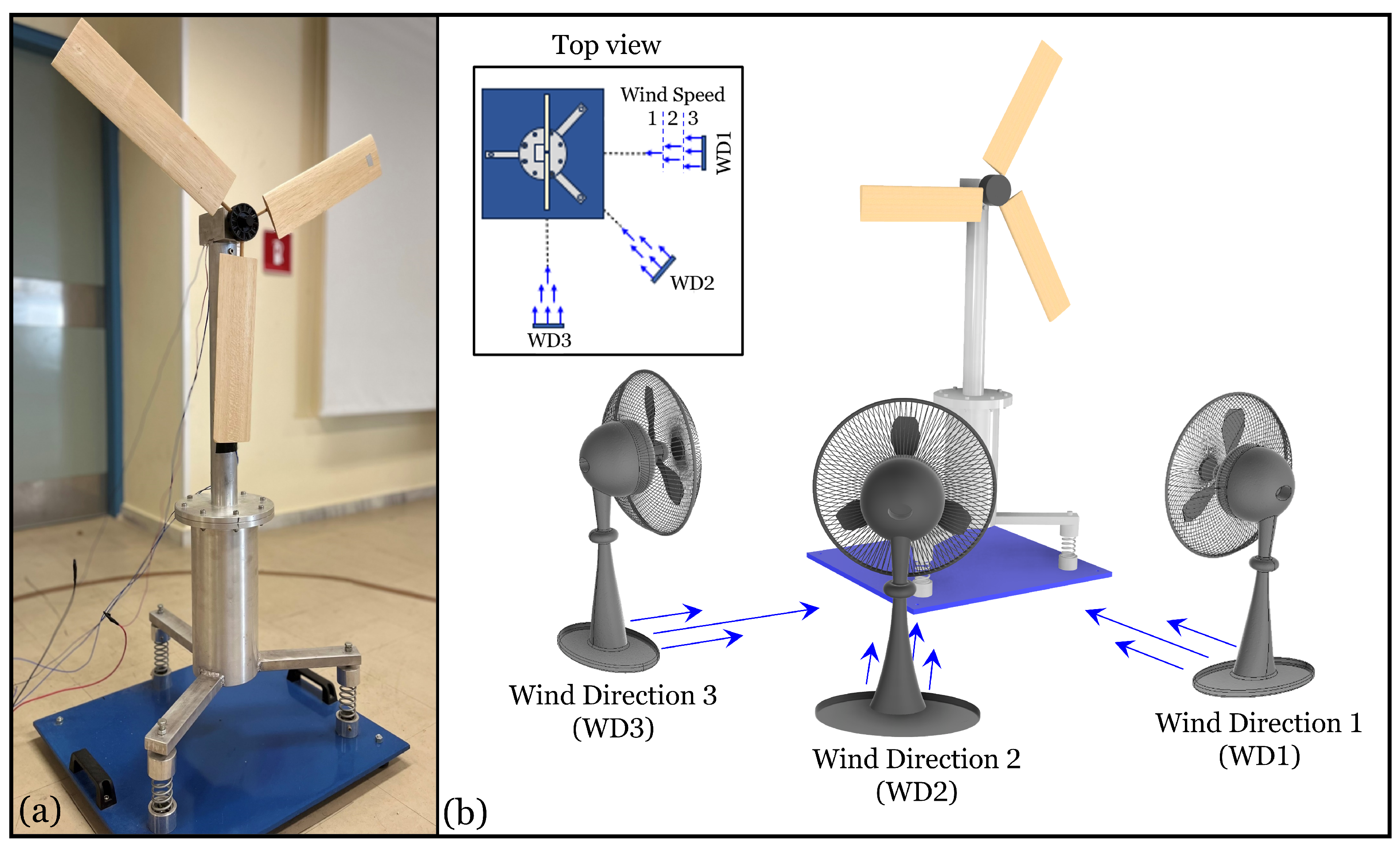
(a) Photo of the lab-scale FWT model and, (b) the FWT under the considered wind directions (WD1, WD2, WD3) and speeds (WS1, WS2, WS3).
Figure 1.
(a) Photo of the lab-scale FWT model and, (b) the FWT under the considered wind directions (WD1, WD2, WD3) and speeds (WS1, WS2, WS3).
Figure 2.
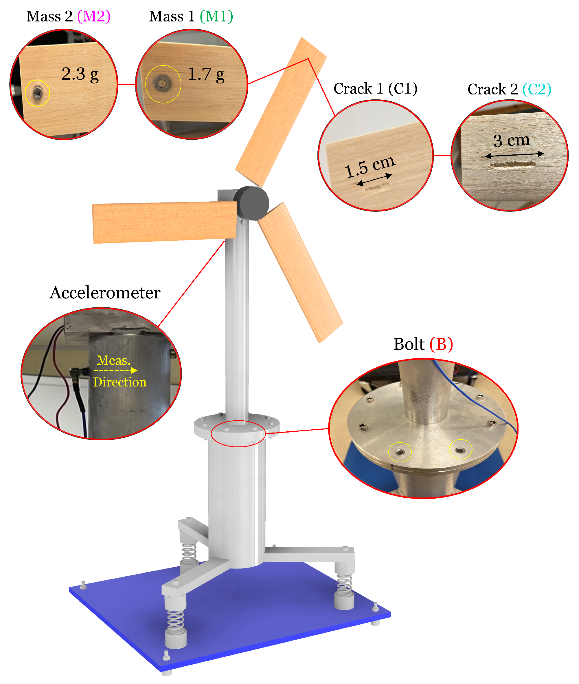
The lab-scale FWT model, the accelerometer position and the considered damage scenarios.
Figure 2.
The lab-scale FWT model, the accelerometer position and the considered damage scenarios.
Figure 3.
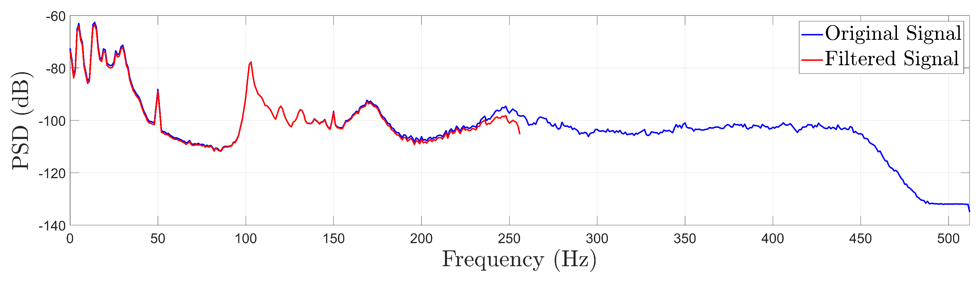
Indicative Welch-based PSD estimate using a vibration signal from the FWT in a healthy state before and after signal filtering and resampling at a frequency of Hz.
Figure 3.
Indicative Welch-based PSD estimate using a vibration signal from the FWT in a healthy state before and after signal filtering and resampling at a frequency of Hz.
Figure 4.
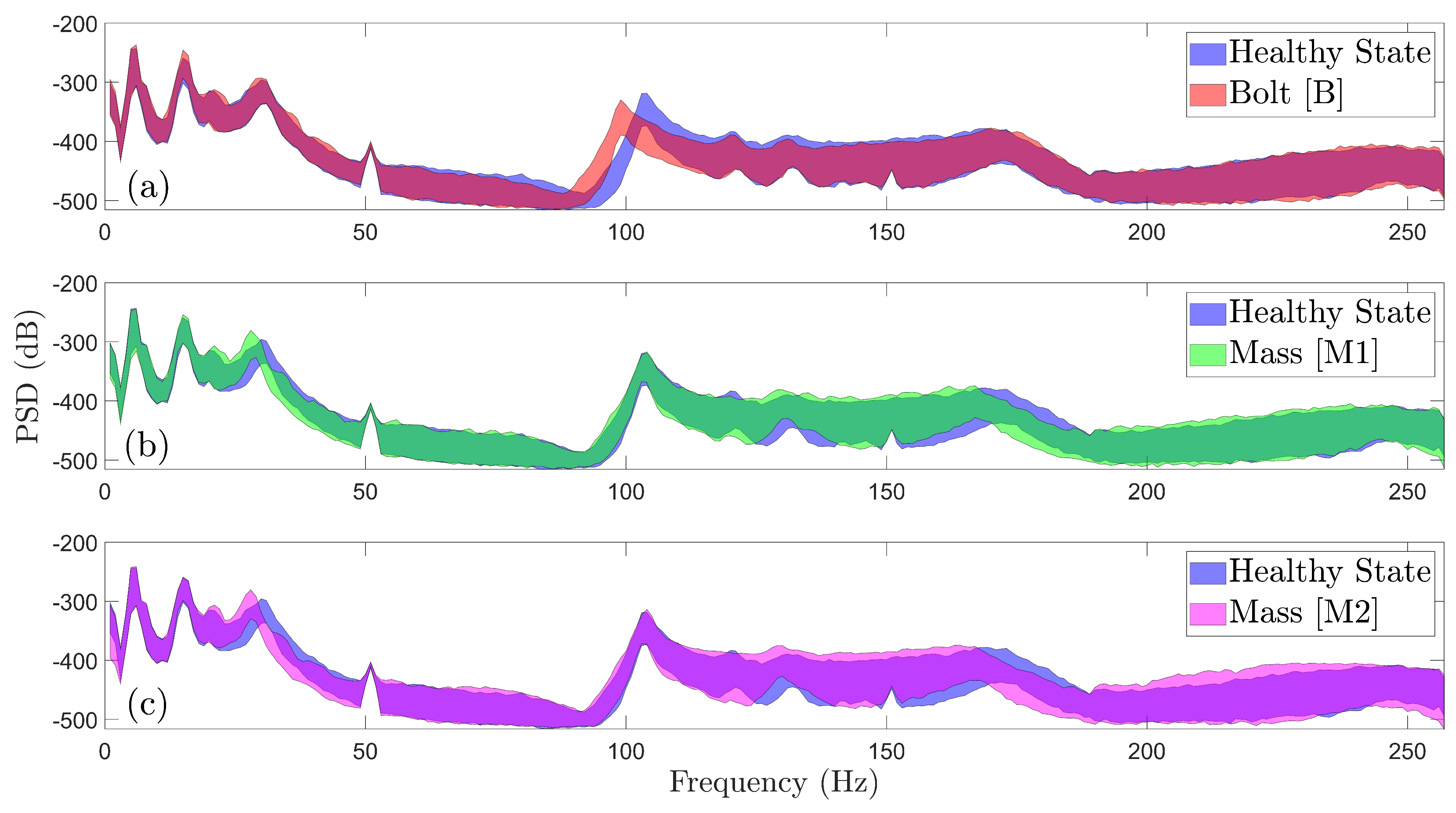
Welch-based PSD envelope estimates under all considered wind speeds and directions of the healthy and damaged FWT (90 signals per health state): (a) Healthy vs Scenario B, (b) Healthy vs Scenario M1 and (c) Healthy vs Scenario M2.
Figure 4.
Welch-based PSD envelope estimates under all considered wind speeds and directions of the healthy and damaged FWT (90 signals per health state): (a) Healthy vs Scenario B, (b) Healthy vs Scenario M1 and (c) Healthy vs Scenario M2.
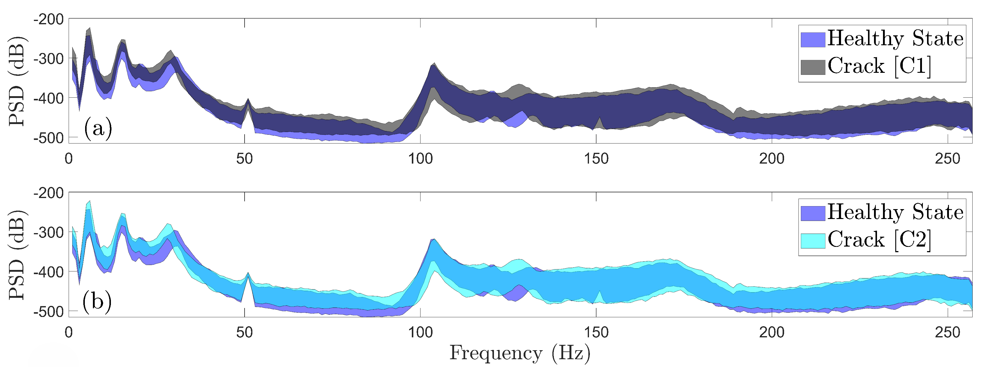
Figure 5.
Welch-based PSD envelope estimates under all considered wind speeds and directions of the healthy and damaged FWT (90 signals per health state): (a) Healthy vs Scenario C1, (b) Healthy vs Scenario C2.
Figure 5.
Welch-based PSD envelope estimates under all considered wind speeds and directions of the healthy and damaged FWT (90 signals per health state): (a) Healthy vs Scenario C1, (b) Healthy vs Scenario C2.
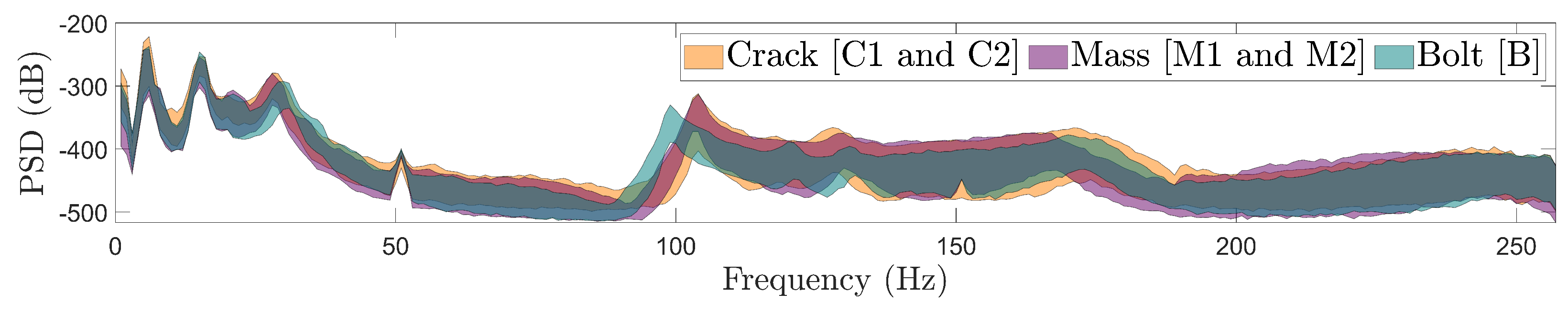
Figure 6.
Effects of different damage types on the dynamics through Welch-based PSD envelope estimates for damage Scenario B (90 signals), for Scenarios C1 & C2 (180 signals), and for Scenarios M1 & M2 (180 signals).
Figure 6.
Effects of different damage types on the dynamics through Welch-based PSD envelope estimates for damage Scenario B (90 signals), for Scenarios C1 & C2 (180 signals), and for Scenarios M1 & M2 (180 signals).
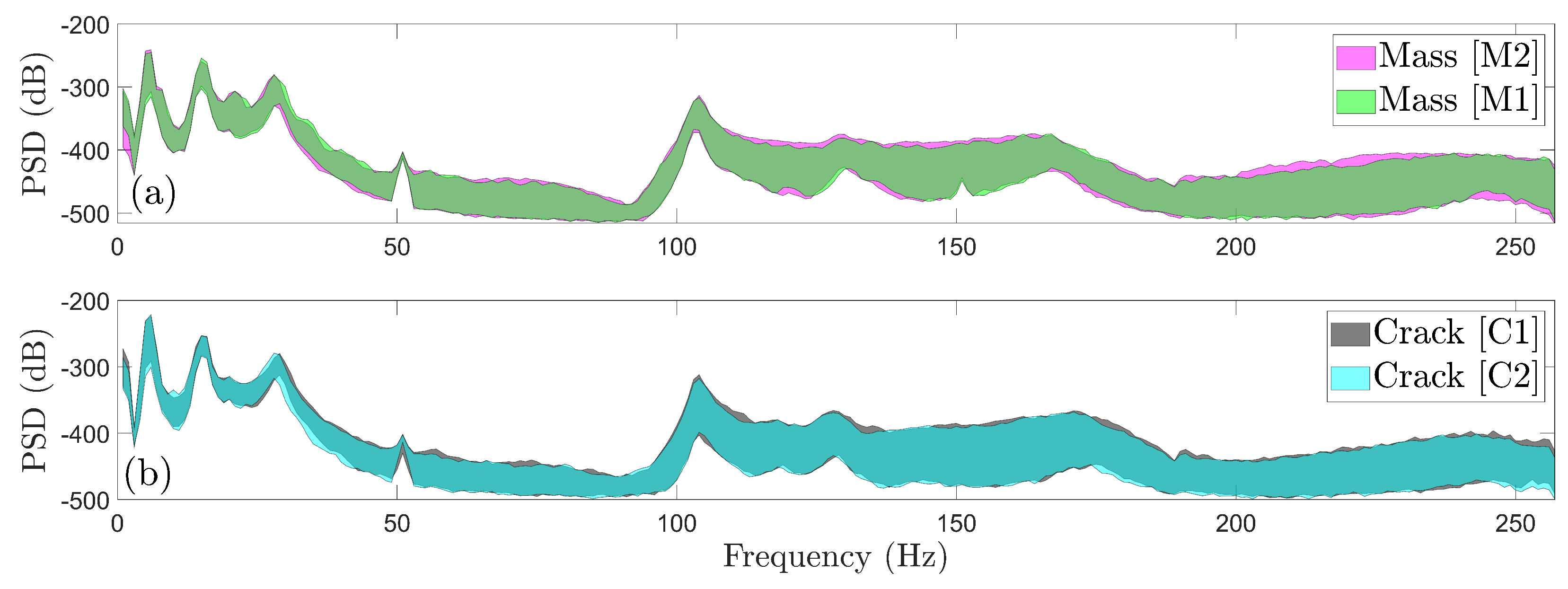
Figure 7.
Effects of different damage severity levels for the same damage type through Welch-based PSD envelope estimates (90 signals per damage severity): (a) Scenario M1 vs Scenario M2, and (b) Scenario C1 vs Scenario C2.
Figure 7.
Effects of different damage severity levels for the same damage type through Welch-based PSD envelope estimates (90 signals per damage severity): (a) Scenario M1 vs Scenario M2, and (b) Scenario C1 vs Scenario C2.
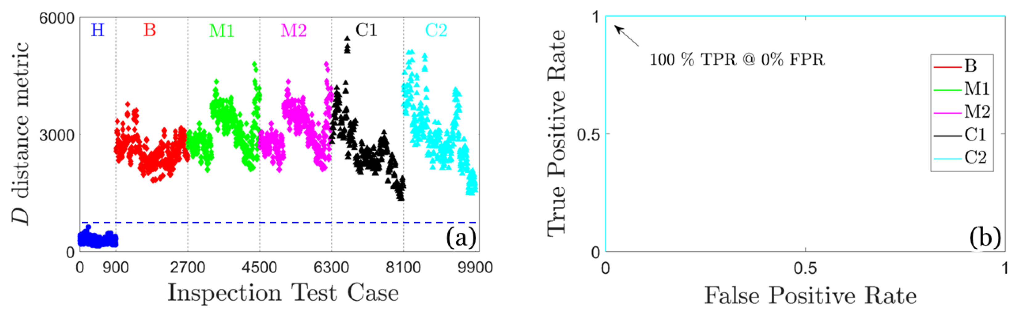
Figure 8.
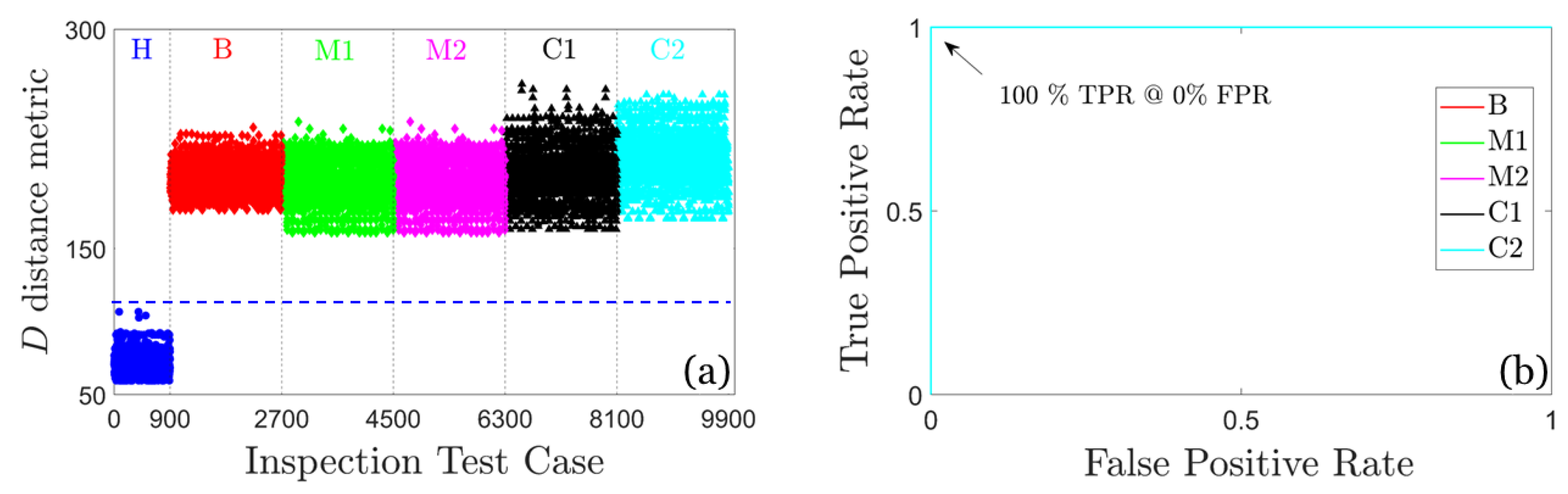
Damage detection results based on the U-MM-AR method: (a) Plot of the distance metric D and (b) corresponding ROC curves; 900 inspection test cases for the healthy FWT and 1800 per damage scenario, 9900 in total. The blue dashed line indicates the user selected threshold.
Figure 8.
Damage detection results based on the U-MM-AR method: (a) Plot of the distance metric D and (b) corresponding ROC curves; 900 inspection test cases for the healthy FWT and 1800 per damage scenario, 9900 in total. The blue dashed line indicates the user selected threshold.
Figure 9.
Damage detection results based on the U-MM-PSD method: (a) Plot of the distance metric D and (b) corresponding ROC curves; 900 inspection test cases for the healthy FWT and 1800 per damage scenario, 9900 in total. The blue dashed line indicates the user selected threshold.
Figure 9.
Damage detection results based on the U-MM-PSD method: (a) Plot of the distance metric D and (b) corresponding ROC curves; 900 inspection test cases for the healthy FWT and 1800 per damage scenario, 9900 in total. The blue dashed line indicates the user selected threshold.
Figure 10.
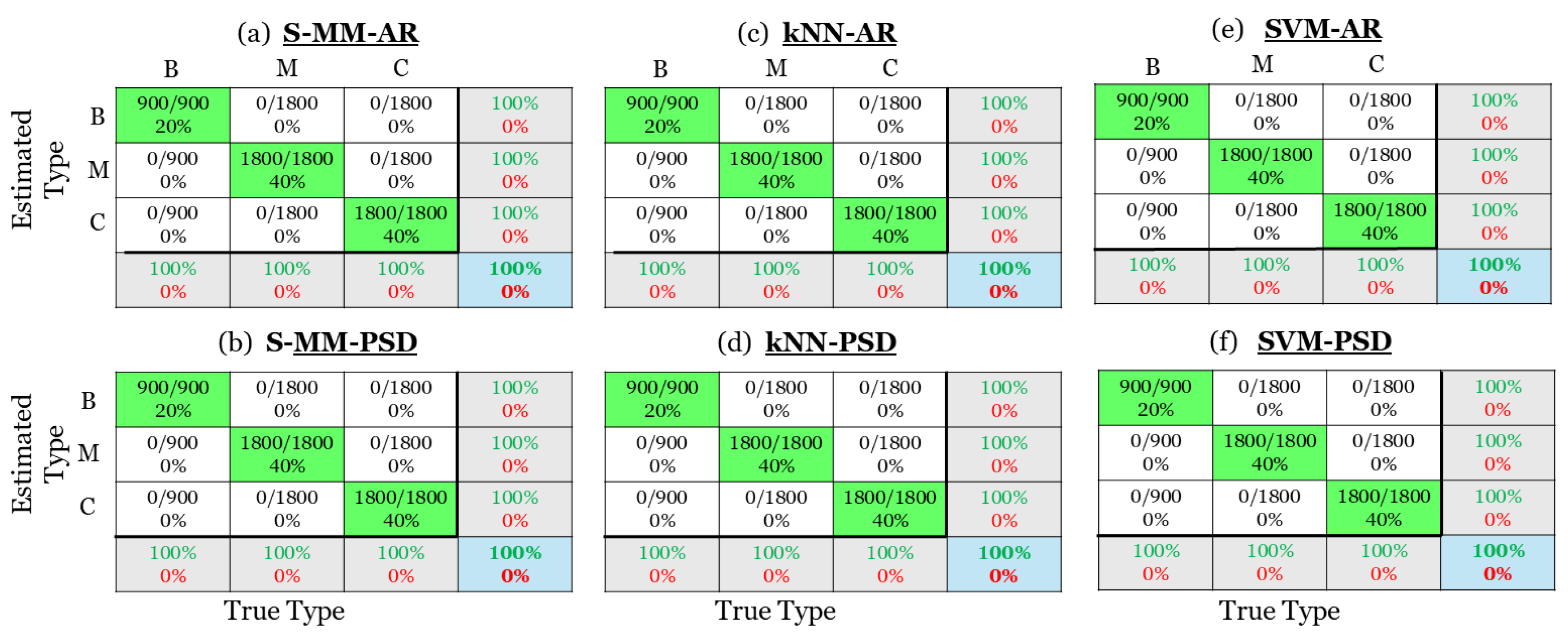
Damage Type identification results via confusion matrices: (a) The S-MM-AR method, (b) the S-MM-PSD method, (c) the k-NN-AR method, (d) the k-NN-PSD method, (e) the SVM-AR method and (f) the SVM-PSD method. Correct identification is indicated by green color and misidentification by red (4500 inspection test cases in total).
Figure 10.
Damage Type identification results via confusion matrices: (a) The S-MM-AR method, (b) the S-MM-PSD method, (c) the k-NN-AR method, (d) the k-NN-PSD method, (e) the SVM-AR method and (f) the SVM-PSD method. Correct identification is indicated by green color and misidentification by red (4500 inspection test cases in total).
Figure 11.
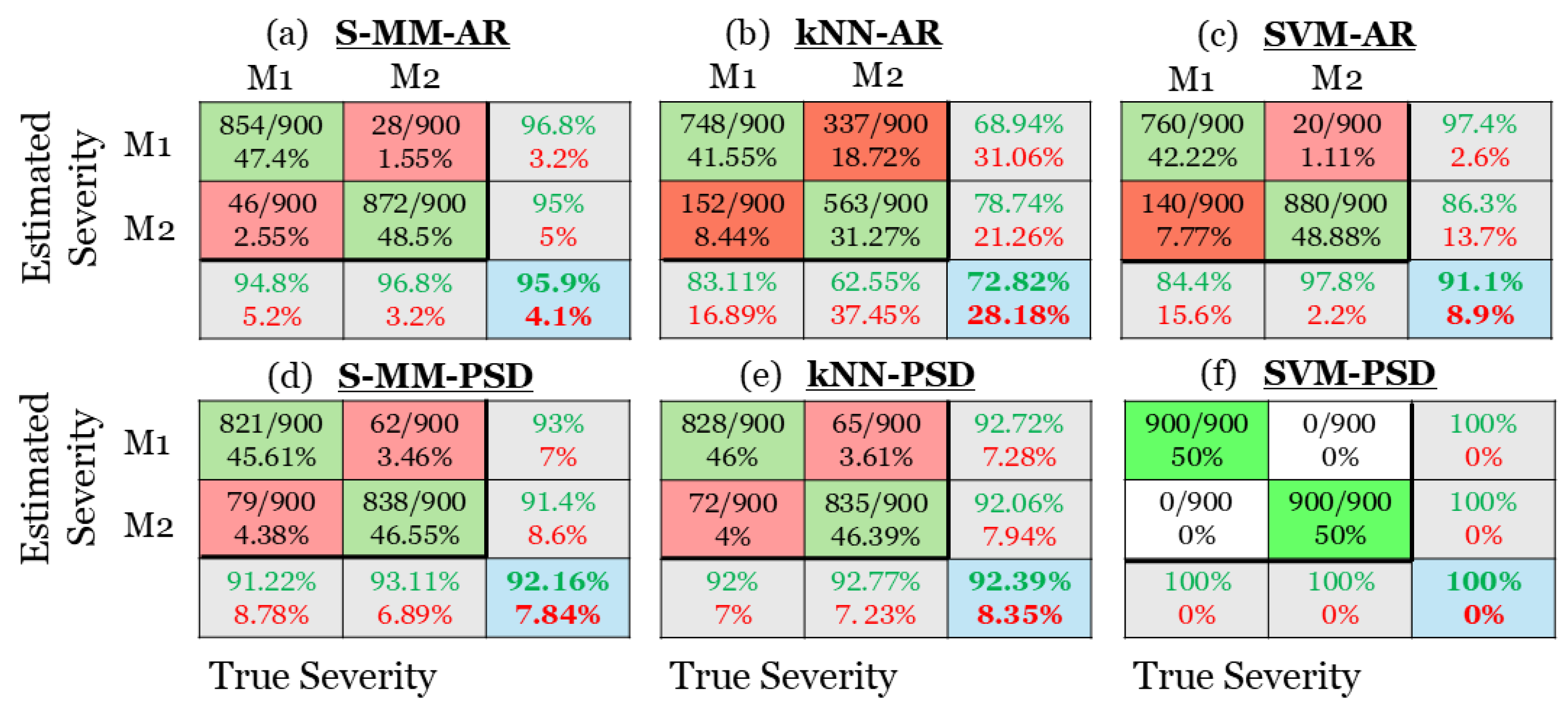
Damage severity characterization results via confusion matrices for Added Mass damage scenario: (a) The S-MM-AR based method, (b) the k-NN-AR based method, (c) the SVM-AR based method, (d) the S-MM-PSD based method, (e) the k-NN-PSD based method, and (f) the SVM-PSD based method. Correct characterization is indicated by green color and mis-charachterization by red (1800 inspection test cases in total).
Figure 11.
Damage severity characterization results via confusion matrices for Added Mass damage scenario: (a) The S-MM-AR based method, (b) the k-NN-AR based method, (c) the SVM-AR based method, (d) the S-MM-PSD based method, (e) the k-NN-PSD based method, and (f) the SVM-PSD based method. Correct characterization is indicated by green color and mis-charachterization by red (1800 inspection test cases in total).
Figure 12.
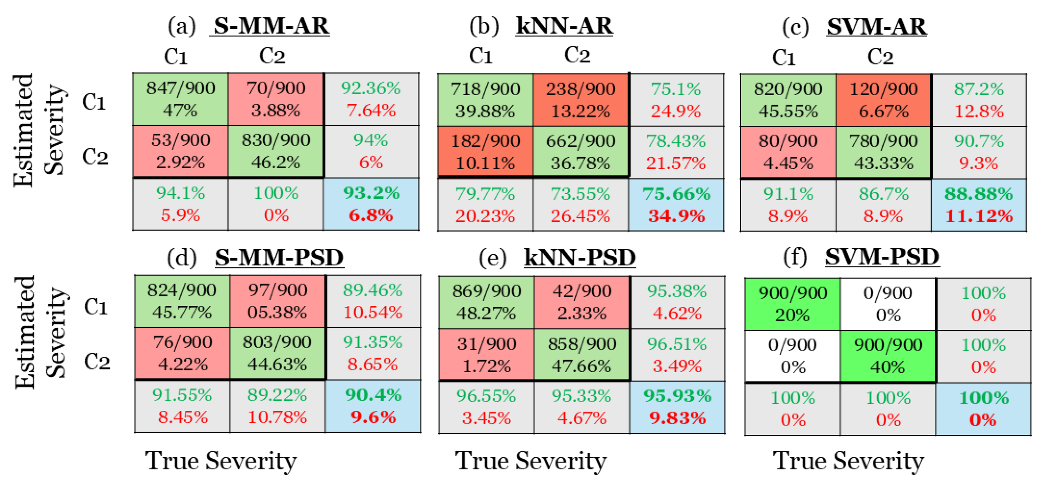
Damage severity characterization results via confusion matrices for Blade Crack damage scenario: (a) The S-MM-AR based method, (b) the k-NN-AR based method, (c) the SVM-AR based method, (d) the S-MM-PSD based method, (e) the k-NN-PSD based method, and (f) the SVM-PSD based method. Correct characterization is indicated by green color and mis-characterization by red (1800 inspection test cases in total).
Figure 12.
Damage severity characterization results via confusion matrices for Blade Crack damage scenario: (a) The S-MM-AR based method, (b) the k-NN-AR based method, (c) the SVM-AR based method, (d) the S-MM-PSD based method, (e) the k-NN-PSD based method, and (f) the SVM-PSD based method. Correct characterization is indicated by green color and mis-characterization by red (1800 inspection test cases in total).
Figure 13.
Summary of severity correct characterization percentages for damage scenarios with added mass () and blade crack (), based on all considered methods.
Figure 13.
Summary of severity correct characterization percentages for damage scenarios with added mass () and blade crack (), based on all considered methods.
Table 1.
Experimental details on the varying wind conditions, the FWT health states and the vibration signals.
Table 1.
Experimental details on the varying wind conditions, the FWT health states and the vibration signals.
| FWT Health State |
Wind Speed (WS) |
Wind Direction (WD) |
No. of Exp. per WS / WD |
Total No. of Exp. |
| Healthy (H) |
{1, 2, 3} |
{1, 2, 3} |
10 / 10 |
90 |
| Bolt (B) |
-//- |
-//- |
-//- |
-//- |
| Mass 1 (M1) |
-//- |
-//- |
-//- |
-//- |
| Mass 2 (M2) |
-//- |
-//- |
-//- |
-//- |
| Crack 1 (C1) |
-//- |
-//- |
-//- |
-//- |
| Crack 2 (C2) |
-//- |
-//- |
-//- |
-//- |
|
Original signals: |
| Sampling rate: Hz; Length: N=30720 samples; Frequency bandwidth: Hz |
|
Pre-processed signals: |
| Sampling rate: Hz; Length: N=15360 samples; Frequency bandwidth: Hz |
| Pre-processing: Low-pass Chebyshev Type I filter & resampling |
Table 2.
Damage detection – details on the performance assessment.
Table 2.
Damage detection – details on the performance assessment.
| Baseline (Training) phase |
|---|
| No. of Rotations |
Healthy State |
Bolt (B) |
Mass 1 (M1) |
Mass 2 (M2) |
Crack 1 (C1) |
Crack 2 (C2) |
| 1 |
|
– |
– |
– |
– |
– |
| 20 |
900 |
– |
– |
– |
– |
– |
| Inspection (Detection) phase |
| 1 |
|
90 |
90 |
90 |
90 |
90 |
| 20 |
900 |
1800 |
1800 |
1800 |
1800 |
1800 |
|
a 5 signals per wind condition. Different signals per phase. |
| No. of training signals per rotation: 45; Total No. of inspection signals: 9900. |
Table 3.
Damage Type Identification - details on the performance assessment.
Table 3.
Damage Type Identification - details on the performance assessment.
| Baseline (Training) phase |
|---|
| No. of Rotations |
Bolt (B) |
Mass (M1, M2) |
Crack (C1, C2) |
| 1 |
|
|
|
| 20 |
900 |
1800 |
1800 |
| Inspection (Identification) phase |
| 1 |
|
|
|
| 20 |
900 |
1800 |
1800 |
|
a 5 signals per wind condition. Different signals per phase. |
|
b 45 signals per damage Type Scenario (5 signals per wind condition). |
| No. of training signals per rotation: 225; Total No. of inspection signals: 4500. |
Table 4.
Damage Severity Characterization of Added Mass damage scenarios - details on the performance assessment.
Table 4.
Damage Severity Characterization of Added Mass damage scenarios - details on the performance assessment.
| Baseline (Training) phase |
|---|
| No. of Rotations |
Mass 1 (M1) |
Mass 2 (M2) |
| 1 |
|
|
| 20 |
900 |
900 |
| Inspection (Severity Characterization) phase |
| 1 |
45 |
45 |
| 20 |
900 |
900 |
|
a 5 signals per wind condition. Different signals per phase. |
| No. of training signals per rotation: 90; Total No. of inspection signals: 1800. |
Table 5.
Damage Severity Characterization of Blade Crack damage scenarios - details on the performance assessment.
Table 5.
Damage Severity Characterization of Blade Crack damage scenarios - details on the performance assessment.
| Baseline (Training) phase |
|---|
| No. of Rotations |
Crack 1 (C1) |
Crack 2 (C2) |
| 1 |
|
|
| 20 |
900 |
900 |
| Inspection (Severity Characterization) phase |
| 1 |
45 |
45 |
| 20 |
900 |
900 |
|
a 5 signals per wind condition. Different signals per phase. |
| No. of training signals per rotation: 90; Total No. of inspection signals: 1800. |
Table 6.
Damage Detection - details on the methods training and inspection phases.
Table 6.
Damage Detection - details on the methods training and inspection phases.
| Method |
Feature |
Feature vector dimensionality |
Distance type |
| U-MM-AR |
AR parameter vector |
80 |
Mahalanobis |
| U-MM-PSD |
PSD estimates |
256 |
Euclidean |
| Baseline (Training) phase |
| AR model estimation via OLS [35] (p. 204), Matlab function:
|
| Selected model: AR(80); BIC: -17.11; Samples Per Parameter (SPP): 192; |
| Condition Number:
|
| Inspection (Detection) phase |
|
U-MM-AR (U-MM-PSD): Detection based on the minimum Mahalanobis (Euclidean) distance |
| User defined threshold: 600 (90) |
Table 7.
Damage Type Identification - details on the methods baseline and inspection phases.
Table 7.
Damage Type Identification - details on the methods baseline and inspection phases.
| Method |
Feature |
Feature vector dimensionality |
Distance type |
| S-MM-AR |
AR parameter vector |
80 |
Mahalanobis |
| k-NN-AR |
-//- |
-//- |
Cosine |
| SVM-AR |
-//- |
-//- |
- |
| S-MM-PSD |
PSD estimates |
256 |
Euclidean |
| k-NN-PSD |
-//- |
-//- |
Cosine |
| SVM-PSD |
-//- |
-//- |
- |
| Baseline (Training) phase |
| AR model estimation via OLS [35] (p. 204), Matlab function:
|
| Selected model: AR(80); BIC: -17.11; Samples Per Parameter (SPP): 192; |
| Condition Number: , k-NN space: Matlab function:
|
| Inspection (Identification) phase |
|
k-NN-AR: Search Method: Exhaustive; No. of Nearest Neighbors: ; BreakTies: Nearest; |
| Weight: Inverse |
|
k-NN-PSD: Search Method: Exhaustive; No. of Nearest Neighbors: ; BreakTies: Nearest; |
| Weight: Equal (no weighting) |
|
SVM-AR: Kernel Function: Quadratic; Kernel scale: 1; Box Constrain level: 1.852; |
| Multi-class coding: One vs All |
|
SVM-PSD: Kernel Function: Gaussian; Kernel scale: 0.008; Box Constrain level: 22; |
| Multi-class coding: One vs All |
| Bayesian Optimization details: |
| Objective function: minimum classification error; Acquisition function: expected-improvement (EI) |
| Objective function evaluations: 30; Number of initial evaluation points: 4, Exploration ratio: 0.5 |
Table 8.
Damage Severity Characterization - details on the methods Baseline and Inspection phases.
Table 8.
Damage Severity Characterization - details on the methods Baseline and Inspection phases.
| Method |
Feature |
Feature vector dimensionality |
Distance type |
| S-MM-AR |
AR parameter vector |
80 |
Mahalanobis |
| k-NN-AR |
-//- |
-//- |
|
| SVM-AR |
-//- |
-//- |
- |
| S-MM-PSD |
PSD estimates |
256 |
Euclidean |
| k-NN-PSD |
-//- |
-//- |
|
| SVM-PSD |
-//- |
-//- |
- |
| Baseline (Training) phase |
| AR model estimation via OLS [35] (p. 204), Matlab function:
|
| Selected model: AR(80); BIC: -17.11; Samples Per Parameter (SPP): 192; |
| Condition Number: , k-NN space: Matlab function:
|
| Inspection (Severity Characterization) phase |
|
1k-NN-AR: Search Method: Exhaustive(Exhaustive); No. of Nearest Neighbors: ; |
| BreakTies: Nearest(Nearest); Weight: Squared Inverse(Inverse) |
|
1k-NN-PSD: Search Method: Exhaustive(Exhaustive); No. of Nearest Neighbors: ; |
| BreakTies: Nearest(Nearest); Weight: Squared Inverse(Inverse) |
|
1SVM-AR: Kernel Function: Linear(Cubic); Kernel scale: 1(1); |
| Box Constrain level: 247(0.715); Multi-class coding: One vs All(One vs All) |
|
1SVM-PSD: Kernel Function: Linear(Gaussian); Kernel scale: 1(951); |
| Box Constrain level: 0.001(883); Multi-class coding: One vs All(One vs All) |
| Bayesian Optimization details: |
| Objective function: minimum classification error; Acquisition function: expected-improvement (EI) |
| Objective function evaluations: 30; Number of initial evaluation points: 4, Exploration ratio: 0.5 |
|
1The values within the (parentheses) correspond to the Blade Crack scenario; The rest values |
| correspond to the Added Mass scenario |