
Submitted:
25 December 2024
Posted:
26 December 2024
You are already at the latest version
Abstract
This study aimed to summarize the results of using the Lee-Carter model and its extensions to predict mortality in Kazakhstan for ten years up to 2033. We analyzed Kazakhstan's age-specific mortality rates, observed annually from 1991 to 2023. Different mortality models were used to predict mortality. Among them Lee-Carter model, Hyndman-Ullah method with regression of scores on exogenous factors, time series analysis methods. The Lee-Carter model and its extensions did not give satisfactory results for predicting mortality in the testing timeframe. Including external socio-economic factors in the model did not improve forecasting accuracy. The accuracy of the forecast increased with a separate analysis of the subpopulations of children and adults. This was because since 1991 in the children subpopulation there has been a pronounced linear downward trend, while in the adult subpopulation, the global trend in mortality dynamics is nonlinear. As a result, it is possible to make forecasts for 7 years with a high degree of accuracy (error <10%) and forecast for the 8th, 9th, and 10th years with a "good" degree of accuracy (error 10-20%). In 2024-2033, a further mortality decline is expected in most age groups. Only in groups over 80 years old is a slight increase in mortality predicted in the coming year, but then a downward trend will be observed again
Keywords:
public health
; mortality
; mortality rate modelling
; time series forecasting
1. Introduction
Age-specific mortality forecasting plays a crucial role in public health planning and healthcare management. By predicting mortality rates across different age groups, policymakers, healthcare providers, and researchers can make informed decisions that improve health outcomes and allocate resources more effectively. The significance of forecasting age-specific mortality rates lies in several key areas:
Mortality prediction allows healthcare systems to anticipate the future demand for medical services, facilities, and healthcare professionals. Accurate forecasts enable health planners to allocate resources more efficiently, ensuring that adequate infrastructure and healthcare services are available to meet the needs of different age groups [1]. In addition, it helps public health authorities design targeted intervention programs. These targeted strategies can help reduce the burden of disease and lower mortality rates in vulnerable age groups [2]. Age-specific mortality forecasting is also essential for actuarial science, particularly in the insurance and pension sectors. [3].
Knowledge in this area provide valuable insights into the potential impact of emerging health threats, such as pandemics, epidemics, or environmental changes. This information helps epidemiologists and public health researchers model the spread and impact of infectious diseases and assess the effectiveness of public health interventions [4]. It also supports to reveal disparities in health outcomes across different demographic and socio-economic groups. By focusing on vulnerable populations, healthcare systems can work towards achieving equity in health outcomes [5].
Another area where mortality data are needed is strategic planning at national and regional levels. Governments can use this information to plan for future healthcare infrastructure needs, budget allocations, and workforce training. Accurate mortality predictions help align health system capabilities with future demographic trends, ultimately enhancing the resilience and sustainability of healthcare systems [6,7].
In the literature available to us, we found only a few works devoted to the issues of predicting mortality in Kazakhstan. Sapin A.M., using the Lee-Carter model, estimated the impact of mortality on the pension system of Kazakhstan. Unfortunately, the author does not provide data on fitting accuracy and forecasting accuracy, so it is impossible to assess how valid the model used is. [4].
For many years, the Lee-Carter mortality forecasting methodology [9] has been the reference method for extrapolative mortality forecasting. The distinctive advantages of the Lee-Carter model are that it incorporates a simple stochastic model with one time-varying parameter; it works relatively well when past trends are linear; and it is able to forecast changes in the age structure of mortality [10].
The Lee-Carter mortality model is widely used to predict mortality and construct life tables. However, despite its popularity, it has a number of shortcomings that are discussed in scientific literature. The main ones are:
- −
- Linear dependence of the mortality trend. The Lee-Carter model assumes that mortality changes linearly over time through the trend parameter kt. However, as shown in a number of studies, the actual process of mortality change may be non-linear. This makes the model ineffective in predicting long-term trends, especially during periods of significant changes in mortality (epidemics, wars, technological breakthroughs in medicine, etc.). [11]
- −
- Limited flexibility for different age groups. The Lee-Carter model uses fixed age parameters αx and βx, which does not always accurately reflect heterogeneous changes in mortality in different age groups. This may lead to inaccurate forecasts, especially for younger or older age groups, whose mortality may change more dynamically or unpredictably [12]
- −
- Insufficient attention to temporal correlation. The Lee-Carter model assumes that the temporal dynamics of the trend kt is modeled using a random walk, which assumes the absence of temporal correlation or other structural changes in the time series. In reality, the mortality trend may exhibit more complex patterns, such as autocorrelation or cyclicity [13]
- −
- Problems with long-term forecasting. Linear extrapolation of the mortality trend may lead to over- or under-predictions over long time horizons. This is because the model does not account for possible changes in the rate of mortality decline or unexpected increases in mortality [14].
- −
- Instability with small data. The Lee-Carter model requires a large amount of data to accurately calibrate the parameters, which can be a problem for small or sparse populations. In small samples, the model may produce unstable or inaccurate results [15]
- −
- For this reason, many extensions of the Lee-Carter model have been developed. The functional approach to data proposed by Hyndman and Ullah was developed as an alternative to the Lee-Carter model. This approach includes higher-order principal components and nonparametric smoothing and provides a more realistic future age structure of mortality [16].
Unlike parametric models, which require explicit assumptions about the underlying structure of the data, the Hyndman and Ullah model can accommodate a variety of patterns in the data, such as different shapes and trends in mortality rates across age groups and over time. This flexibility makes it suitable for a wide range of populations and data sets with different mortality dynamics.
Using Functional Principal Component Analysis (FPCA), the model reduces the complexity of multivariate mortality data to a few principal components that capture the most significant changes. This approach simplifies the modeling process and reduces noise, resulting in more accurate and interpretable forecasts [17]. The model provides more robust forecasts than models that only consider linear trends or are restricted to certain parametric shapes [4]. The model is relatively simple to implement, and the resulting principal components can be interpreted in terms of changes in the level, slope, and curvature of mortality rates over time. This interpretability is a key benefit for population researchers and policymakers who require clear and actionable insights from mortality forecasts.
For forecasting based on FPCA, various methods are used, among which are autoregressive models (ARIMA), moving average or exponential smoothing (ETS) models, regression models, machine learning, etc. The use of a particular method depends on the mortality structure, transition processes in demographic and epidemiological processes, the age structure of the population, the state of the health care system and the socio-economic conditions of the population. [11,12,18].
The aim of this study was to summarize the results of using the Lee-Carter model and its extensions taking into account socio-economic factors to predict mortality in Kazakhstan for ten years up to 2033. For this purpose, at the first stage we analyzed the main trends in mortality among different age groups since the formation of the Republic of Kazakhstan in 1991. Then we used the Lee-Carter model and its modification proposed by Hyndman and Ullah. The forecast was carried out with and without considering the influence of external factors. The best forecasting results were obtained by us with a separate analysis of the subpopulation of children and adults, in which different time trends were observed in previous years. When forecasting 10 years ahead, the error was no more than 20% for all age groups.
2. Materials and Methods
2.1. Data
We considered Kazakhstan age-specific mortality rates, observed annually from 1991 (since the creation of an independent state) to 2023, obtained from website stat.gov.kz. Actual mortality rates are estimated as the ratio of number of deaths to the midyear population size for 5-year (0, 1-4, 5-9, .... 80-84, 85+) age groups.
Figure 1 shows the dynamics of the total mortality rate in this period. We selected 1991-2013 years as training timeframe (fitting period) and 2014-2023 years as testing timeframe.
2.2. Lee Carter Model (LC)
The model’s basic premise is that there is a linear relationship among the logarithm of age-specific mortality rates and two explanatory factors: the initial age interval x, and time t. The equation that describes this fact is as follows:
where:
mx,t is the mortality rate for age x at time t,
ax is average mortality at age x over time,
bx is the deviation in mortality due to changes in the kt index,
kt is the time-varying coefficients, reflecting the temporal variation in mortality,
εx,t is the error term
The parameters of the Lee–Carter model were estimated using singular value decomposition (SVD) method to a matrix of centered log mortality rates [9]. Then we utilized the ARIMA method to predict the time index kt.
2.3. Hyndman-Ullah Model (HU)
This model can be expressed as:
where:
mx,t is the mortality rate for age x at time t,
μ(x) is the mean function of mortality over time,
βk(x) are the functional principal component (FPC) loadings, capturing age-specific patterns of mortality change,
κk,t are the time-varying coefficients (scores) associated with each FPC, reflecting the temporal variation in mortality,
ε(x,t) is the error term.
Following the application of the Hyndman-Ullah model, we performed Functional Principal Component Analysis (FPCA) to further reduce the dimensionality of the mortality data and retain the most significant patterns. The FPCA approach identifies a set of orthogonal basis functions that explain the majority of the variance in the log-mortality rates, allowing us to capture the underlying trends and structures in the data with fewer components.
We estimated the model using different basis functions:
- −
- Automatic extraction orthonormal basis functions directly from the data through FPCA. This ensures that the basis functions adapt to the underlying structure of the mortality data (package ftsa in R)
- −
- B-splines
- −
- Fourier basis
- −
- Cubic splines
The FPCA-transformed components (scores κk,t) reflect the evolution of mortality trends over time and provide a compact representation of the original high-dimensional data. There were used several methods to forecast the principal component scores:
- −
- ARIMA [19]
- −
- Linear Regression (LR)
- −
- Linear Regression with Added Stochastic Oscillations (LR+A) is a forecasting approach that combines the deterministic modeling capabilities of linear regression with the flexibility of stochastic components to account for random fluctuations or oscillatory behaviors in the data. In our study, the stochastic component is described using ARIMA [20].
- −
- The Generalized Additive Model (GAM) is an extension of linear and generalized linear models that accommodates nonlinear relationships between predictors and the response variable. It constructs the model by additively combining smoothing functions for the predictors, making it a powerful tool for modeling complex dependencies. [21].
- −
- The ETS model, also known as Exponential Smoothing State Space Model, is a time series forecasting approach that captures three key components: Error, Trend, and Seasonality. The model’s formulation considers different combinations of these components, which can be either additive or multiplicative [22].
2.4. Hyndman-Ullah Method with Regression of Scores on Exogenous Factors
To account for the influence of exogenous factors on mortality, we applied a Two-Step Functional Principal Component Regression (FPCR) approach [23,24]. In the first step, we performed FPCA to decompose mortality rates into principal components. In the second step, instead of extrapolating scores only from their internal dynamics, we use information about exogenous factors to make a more accurate forecast. For each score a regression is performed on external factors:
α – is intercept
γ1, γ2, γ3 … γn. are regression coefficients
z1, z2, z3 … zn are exogenous factors
ɛt is error
As exogenous factors, we selected population size (Popul), density of medical doctors (Doctors) и gross domestic product per capita (GDP).
In our analysis, we employed the bootstrap sampling method to artificially augment the dataset and assess the robustness of our regression models. Bootstrap is a statistical technique that involves sampling with replacement from the original dataset to create new datasets of the same or different size. This method is particularly useful when the original sample size is small and it is not feasible to obtain additional data [25].
2.5. Model Validity
To validate a model in each time frame, we compared the model output to real data and calculated accuracy metrics:
Absolute Percentage Error (APE)
where
- real data
- forecasted data
Mean Absolute Percentage Error (MAPE)
Model accuracy was evaluated as highly accurate (MAPE%<10), good (MAPE%: 10-20), reasonable (MAPE%: 20-50), and inaccurate forecasting (MAPE%>50) [26].
3. Results
3.1. Analysis of Mortality Rates in Kazakhstan
Figure 2 shows the logarithmic mortality rates for Kazakhstan from 1991 to 2023. In the first years of independence, there was an increase in mortality, which we associate with the difficult socio-economic situation that arose after the collapse of the Soviet Union. Then there was a period of stabilization, and in the early 2000s, the government took intensive measures to improve the well-being of people and develop the health care system. All this has led to the fact that in recent years there has been a decrease in mortality among all age groups.
If we analyze mortality rates by age, we can see a tendency to increase after 15 years. The rate of increase is relatively high for age groups from 15 to 29 years but slows down after 30 years. Mortality reaches its peak in the oldest age group, over 85 years.
3.2. Fitting Whole Population Mortality Data into the Lee-Carter Model
Figure 3 presents the calculated values of the LC model parameters. The coefficient аx is calculated as the average value for all age groups for all years. Based on this parameter, it can be concluded that high mortality is observed among newborns, then it reaches a minimum in the age range of 10-14 years; and increases in subsequent age groups.
The coefficient bx obtained from the SVD, on the one hand, estimates the sensitivity of mortality for each age to changes in the overall time trend. When analyzing the graph, it becomes apparent that certain age groups show higher changes in mortality rates, as indicated by their respective bx values. In particular, the rate of change is higher for age groups 1–4, followed by a slight decrease at 4-9. It then peaks in the 20–24 age group and starts to decline again. The next maxima are observed at 50–54 and after 85 years. This comprehensive visualization allows us to understand the dynamic patterns of change in mortality rates in different age groups over the observed period.
On the other hand, this coefficient reflects the extent to which the time trend kt affects mortality for a particular age group. If bx is negative, then a decrease in kt leads to an increase in mortality for a given age group, while an increase in kt leads to a decrease. Figure 3 shows that bx takes negative values in almost all age groups. The product of these two coefficients was positive and increased until 1996, then began to decrease and stabilize for some time, and since 2008 it has become negative. That is, we can conclude that before 1996, Kazakhstan experienced an increase in mortality, then some stabilization, and then a clear downward trend can be traced until 2023. All this indicates the presence of a nonlinear trend in the mortality dynamics. Apparently, this was the reason for the insufficient accuracy of forecasting on the testing timeframe (2014 - 2023), since, as already noted, one of the shortcomings of the Lee-Carter model is its linear nature. Table 1 shows the assessment of the fit accuracy and the accuracy indicators of the model on the testing timeframe. In general, the fit results can be considered satisfactory (on average MAPE = 7.23%), although in infant groups the error was 14-16%. But on the testing timeframe certain age groups error reached 42-43% (1-4, 30-34 groups). On average for all groups MAPE was 15.8%.
3.3. Fitting Whole Population Mortality Data into the Hyndman and Ullah Model
In this model more than one principal component is used. Higher order terms of the principal component decomposition improve the LC model because these additional components capture non-random patterns, which are not explained by the first principal component. Using functional principal component analysis (FPCA), a set of curves is decomposed into orthogonal functional principal components and their uncorrelated principal component scores.
Various orthogonal functions can be used as basis functions. The peculiarity of the ftsa package is that by default, the model extracts orthonormal basis functions directly from the data through FPCA. Scores were forecast using the ARIMA method with automatic selection of the best parameters. After that, we independently installed B-splines, Fourier basis, and Cubic splines as basis functions.
At the first stage, we included all 19 age groups in the analysis. The model was fitted to Kazakhstan data from 1991 to 2013. Regardless of the type of basis functions, we obtained the same result for the contribution of the first three principal components. The basis functions explain 67%, 27.3% and 2.5% of the variation respectively. The parameter µ(x) in the Hyndman and Ullah model is analogous to the coefficient ax in the Lee-Carter model, that is, it shows that mortality is high among newborns, then decreases and increases again after 5 years (Figure 4).
The first principal component β1(x) characterizes the contribution of each age group to the overall mortality trend. In the children’s subpopulation, this contribution decreases with age, while in the adult subpopulation, it increases. β1(x) together with the scores k1t determine how this contribution changes in different age groups over time. These two values characterize the interaction between age and time trends. According to them, the global mortality trend is expressed in its growth until approximately 1998, then a slow decline until 2006 and an acceleration of this trend thereafter.
The second component β2(x) explains local changes in mortality in a separate age group associated with the influencing factors characteristic of it. Such changes are observed in the 0-4, 20-24 and 50-54 age groups. According to the scores k2t values, before 2006 these were the factors that increased mortality, but later mortality was influenced by factors that reduced it.
The contribution of the third component is only 2.5% and its interpretation is not obvious. Table 2 provides summaries of the point fitting and forecasting accuracy based on the MAPE of age group mortality rates averaged over different years in the training and testing periods. We found that regardless of the type of basis functions, the fitting results were the same. HU methods tend to perform better accuracy than the LC methods. In the training timeframe, the MAPE values ranged from 1.39% to 7.56% for different age groups. On average, the fitting accuracy was 97%.
However, the accuracy of forecasting was low on the test sample. The average value of MAPE for all age groups is 25.5%. The greatest discrepancy between the actual and forecast data was found in children’s age groups: in the [0] group MAPE = 94.4%, in the 1-4 age group MAPE = 49.1%, in the 5-9 age group MAPE = 29.7%.
3.4. Influence of External Factors on Forecasting
External socio-economic factors have a major impact on mortality, among which the most important are the state of the health care system and the level of well-being of the population. In this regard, after identifying the main components, we predicted the principal component scores for the test period, considering them as a linear regression from the predictors of population size, density of medical doctors and gross domestic product per capita (Table 3).
As already indicated, the first component β1(x) together with the scores k1t determine how this contribution changes in different age groups over time. Based on the data in Table 3, we can estimate the relationship of k1t with external factors. The greatest influence is exerted by GDP, almost 79% of the variance falls on it. The regression coefficient of this factor has a negative value and, accordingly, this indicates the opposite effect of this factor on mortality. That is, an increase in GDP leads to a decrease in mortality. The next most important is the density of doctors (20.83% of the variance). The influence of population size is statistically insignificant.
The second principal component characterizes individual age groups mortality impact on the global trend. Over time, these impacts may change, which is reflected using the score k2t. External predictors influence degree on this coefficient can be assessed using the regression analysis data presented in Table 3.
According to these data, the greatest impact is exerted by population size (54.83% of variance) and GDP (44.97% of variance). The factor of provision with medical personnel does not have a significant impact. After obtaining the regression equations on the training timeframe, k1t and k2t were forecasted for 10 years (2014 - 2023) using the ARIMA method without external factors and the linear regression method with external factors. The results are presented in Figure 5. The dynamics of the coefficients calculated for the entire analyzed period 1991-2023 are also shown.
3.4.1. Forecasting First Component Score
The gray line in Figure 5A, reflecting the dynamics of first component scores over the entire observation period, demonstrates a consistent decrease in this value on the 2014-2023 timeframe. The regression analysis showed that the contribution of GDP to the total variance (i.e., its impact on the first component) is the largest among all factors. However, if on the training timeframe GDP demonstrated almost linear growth, then on the testing timeframe the dynamics changed to non-linear (Figure 6A). This affected the forecasting of first component scores. The green dotted line in Figure 5A shows the non-linear nature of the forecast.
In the same Figure 5A, the blue dotted line is the result of forecasting using the ARIMA method (excluding external factors). In this case, the forecast data are closer to the actual data.
3.4.2. Forecasting the Second Component Score
The dynamics of the second component score on the training timeframe perform us local mortality changes influence on overall mortality. In first it weakens (the score value approach zero), then increases in the period from 1996 to 2007 (the score value become positive), and then decreases again starting in 2007. The second component is more influenced by the population size, which decreased until the early 2000s and has been growing in recent years (Figure 6B). This factor enters the regression equation with a minus sign, so on the test timeframe it is predicted that population growth reduces the value of the second component score.
GDP also had a strong positive relationship with the second component on the training timeframe, but apparently this relationship weakened in the test period, since GDP was nonlinear in these years. As a result, we believe that the main influencing factor was the growing population, which led to a decrease in k2t (green line in Figure 5B). In reality decline was slower (gray line), and this difference in the rate of decline became the source of the forecast error. It should be noted that in the analyzed period, the doctors density in the republic has not undergone significant changes (Figure 6C). Therefore, the influence of this factor was insignificant.
After forecasting the first and second component scores on the testing timeframe, mortality for each age group was calculated and compared with real data. According to the data in the Table 4, considering external factors did not lead to an improvement in forecasting.
3.5. Subpopulation Analysis
We found that the dynamics of the mortality rate in children in 1991-2023 had its own characteristics. In the age groups (0, 1-4, 5-9, 10-14), there was a clear linear downward trend with some fluctuations in individual years (the Figure 7A shows examples of changes in mortality in the child subpopulation). In adults, mortality increased in the first years, then a period of relative stabilization set in, and starting in 2007, a downward trend emerged (the Figure 7B shows examples of changes in mortality in the adult subpopulation).
Based on these results, we analyzed mortality prediction models separately for the subpopulations of children and adults.
3.5.1. Fitting Adult Subpopulation Mortality Data into the Hyndman and Ullah Model
The adult subpopulation included age groups 15-19 and older. In the ftsa package, the extracts orthonormal basis functions directly from the data through FPCA and ARIMA forecasting mode was used. The accuracy of the fit on the training timeframe was quite high, the average MAPE value for all age groups was 2.29%. On the testing timeframe the forecasting accuracy averaged about 90%, which also satisfied us (Table 5).
3.5.2. Fitting Child Subpopulation Mortality Data
The children’s subpopulation included four groups and therefore we could not use the Hyndman and Ullah model due to insufficient data. Therefore, a time series analysis model was selected for each group separately. Among them are ARIMA, ETS, GAM, LR, LR+A.
3.5.4. Mortality Prediction Model for Group (0)
Table 6 and Figure 8 shows that in the test area the best prediction result was obtained using the LR+A method - on average, the APE was 14.17%. However, if we look at the years, the ARIMA results are preferable, since in the first five years there is high prediction accuracy (MAPE<10%), while according to the LR+A method, the prediction accuracy in the first five years was in the range from 10 to 20%.
3.5.5. Mortality Prediction Model for the 1-4 Age Group
For this group, the GAM method (Table 7, Figure 8) showed the best result on the test section. The average APE value was 17.13%. High prediction accuracy (APE<10%) was observed in the first five years. In the following two years, the results can be considered satisfactory. In general, this method shows the possibility of making predictions for 7 years (MAPE = 8.7%).
3.5.6. Mortality Forecasting Model for the 5-9 Age Group
In the 5-9 age group, the best results were shown by the linear regression and regression with ARIMA methods (Table 8, Figure 8). The average forecast error in the 10-year test section was 8.23%. Model accuracy was evaluated as highly accurate in the timeframe from 2014 to 2020. In other years, the forecast accuracy was at least 80%.
3.5.7. Mortality Forecasting Model for the 10-14 Age Group
As can be seen from Table 9 and Figure 8, in the 10-14 age group, linear methods also showed a good result in predicting mortality. Highly accurate was demonstrated by the model when forecasting mortality in 2015 and on the timeframe from 2018 to 2023 (APE <10%). The forecast for other years had an error from 11.48% to 14.29%.
4. Discussion
The Lee-Carter model and its modifications are particularly useful when global trends affecting all age groups need to be considered, consistency of predictions across ages is important, and an interpretable and efficient model is required.
This paper presents an applied approach to forecasting age-specific mortality series using principal component analysis and comparing the predicted continuous distribution rather than the observed discrete values. In general, Hyndman and Ullah discussed that this approach yields better forecasting results than the Lee and Carter approach to mortality forecasting. However, the success of a particular method often depends on the specific dynamics of the mortality rate in a given country and on the quality of the available data. We examined this method using data on annual age-specific mortality among the population of Kazakhstan. Our main goal was to forecast mortality in Kazakhstan for ten years up to 2033, since this is important both in economic and social aspects.
Estimates of the parameters of both models indicate that in Kazakhstan age-specific mortality is similar to the one observed in most of the countries in which this analysis was carried out – high mortality at birth, a decrease in children’s groups and an increase with age in the adult subpopulation. Both models show a peak in mortality in the 0-4, 20-24 and 50-54 age groups. Overall, mortality dynamics are nonlinear, and this may be the reason why both models yielded poor prediction results on the testing timeframe.
Over the past 15 years, Kazakhstan has seen a consistent decline in mortality. This is due to the overall growth of economic and social well-being and the implementation of various programs to improve health services to the population. Special measures have been developed and implemented in the field of motherhood and childhood. In this regard, we assumed that considering external factors in the model would improve its predictive ability. Unfortunately, we were limited in the choice of these external factors, since statistical data on the state of the economy in general, and healthcare in particular, began to be officially published only since the early 2000s. We had access to data on population, GDP, and the provision of medical specialists. However, including these factors in the model did not improve forecasting. One of the reasons is the change in GDP during periods of crisis in the economy. In 1991-2013, GDP showed confident growth, and its correlation with mortality was high, more than -0.8. Subsequently, there were periods of both a decrease and an increase in GDP, so the correlation coefficient decreased to -0.11.
Subsequently, we suggested that our forecasting failures are due to the peculiar properties of the dynamics of mortality in different subpopulations.
The LC model assumes that mortality changes linearly over time through the trend parameter kt. In the HU model, if the trends in age groups differ greatly (for example, one age group has a linear trend, and another - a non-linear one), FPCA may inadequately identify common trends, and some of the significant dynamics will remain in the residuals ɛ(x,t). Particularly high error values were obtained in children’s groups, up to 15 years old. In this regard, we analyzed the mortality curves separately in the children and adult subpopulations. We have seen that in the children subpopulation since 1991 there has been a pronounced linear downward trend, while in the adult subpopulation the global trend in mortality dynamics is nonlinear. Based on this, it was decided to conduct the analysis separately among children and adults. As a result, in the adult subpopulation, the Hyndman and Ullah model showed satisfactory results both at the fitting and testing stages.
Only four groups were included in the children subpopulation. The use of small samples in the Lee-Carter and Hyndman and Ullah models is associated with a number of problems:
- −
- small samples provide little information about the age structure of mortality, making it difficult to model complex interactions. As a result, important information about mortality in adjacent ages may be missed, especially if the mortality dynamics vary greatly between age groups.
- −
- a small sample is more sensitive to noise and the probability that random fluctuations in mortality will be interpreted by the model as significant trends increases.
- −
- the amount of information available for identifying time trends is limited, which leads to uncertainty in forecasts. Forecasts may be unstable or unrealistic.
- −
- with a small number of groups, interpretation of components becomes difficult, since they may not have a clear biological or demographic meaning.
- −
- In this regard, it was decided to conduct the analysis separately in each group using different time series methods. We assessed which methods give the smallest ARE error on the test sample.
In the period from 1995 to 2013, the decline in mortality in childhood age groups occurred with high intensity, the annual rate of decline over these years averaged 5.1%. Apparently, this was due to the general improvement in the economic situation in Kazakhstan and the implementation of a number of state programs in the field of healthcare, and especially in the field of maternal and child health. In subsequent years, this rate slowed down to 3.9%. The models used “could not” adequately reflect this inflection point, “trying to maintain the gained rate” for the future, which led to a mismatch between the real and model data. This mismatch increased as the forecasting periods increased. We selected the models that showed the greatest accuracy. They turned out to be ARIMA for the age group (0), GAM for the group (1-4), LR for the groups (5-9) and (10-14). Using them, it is possible to make forecasts for 7 years with a high degree of accuracy (error <10%) and forecast for the 8th, 9th and 10th years with a “good” degree of accuracy (error 10-20%).
5. Conclusions
Based on the selected models, mortality in Kazakhstan was forecasted until 2033.
As Figure 9 shows, we expect further declines in mortality in most age groups. Only in groups over 80 years old is a slight increase in mortality predicted in the coming year, but then a downward trend will be observed again. The forecast data are given in the Supplementary materials.
Despite the importance of the results obtained, our study is not without a number of limitations. The article did not present data separately for female and male populations. Preliminary analysis showed that there are no significant gender differences in the age and time structure of mortality in Kazakhstan. In order not to overload our article with numerous tables and figures, we decided to consider this aspect in more detail in future publications.
As already mentioned above, over the past 18 years, the Republic has seen a consistent decrease in mortality in all age groups. Obviously, this is happening under the influence of controllable socio-economic factors. For future work, taking these factors into account may improve model fit and increase prediction accuracy.
In our study, the training timeframe included 23 years starting in 1991, from the moment of the formation of the independent Republic of Kazakhstan. At the same time, the WHO website contains data on mortality in Kazakhstan starting from 1950, when the Republic was still part of the USSR. Perhaps, using these data will lead to different results. This aspect can also be considered in future works.
Supplementary Materials
The following supporting information can be downloaded at website of this paper posted on Preprints.org, Table S1: Kazakhstan mortality historical data, Table S2: Kazakhstan mortality forecasting data up to 2033.
Funding
This research received no external funding.
Authors’ Contributions Conceptualization
BK, BO; Data curation: all authors; Formal analysis: BK, RZ; Methodology: BK, BO, MM; Supervision: BK, BO; Validation: MM, RZ; Visualization: MM, RZ; Writing–original draft: all authors; Writing–review and editing: all authors. All authors read and approved the final manuscript.
Institutional Review Board Statement
Not required ethical approval.
Informed Consent Statement
Not applicable
Data Availability Statement
This published article, along with its supplementary files, contains all the data generated or analyzed during the study. The data supporting the findings of this study are available from the https://www.who.int, statgov.kz, worldbank.org ftsa package is available in https://github.com/cran/ftsa
Conflicts of Interest
The authors have no conflicts of interest to declare.
References
- European Commission, Dealing with the Impact of an Ageing Population in the EU (2009 Ageing Report).
- Murray Paul, Jeffrey L. Bohn. Mortality improvement: understanding the past and framing the future, 2018.
- Carone G, Eckefeldt P, Giamboni L, Laine V, Pamies S. Pension reforms in the EU since the early 2000’s: achievements and challenges ahead. European Economy Discussion Papers 42. Brussels: Directorate-General for Economic and Financial Affairs (European Commission), 2016.
- Janssen F. Advances in mortality forecasting: introduction. Genus. 2018;74(1):21, s41118-018-0045-0047. [CrossRef]
- Kraftman L, Hardelid P, Banks J. Age specific trends in mortality disparities by socio-economic deprivation in small geographical areas of England, 2002-2018: A retrospective registry study. The Lancet Regional Health - Europe. 2021;7:100136. [CrossRef]
- Li T, Zhang S, Li H. Research on social and economic factors influencing regional mortality patterns in China. Sci Rep. 2024;14(1):10614. [CrossRef]
- Christensen K, Doblhammer G, Rau R, Vaupel JW. Ageing populations: the challenges ahead. The Lancet. 2009;374(9696):1196-1208. [CrossRef]
- Sapin A. Forecasting mortality for Kazakhstan and assessing it’s impact on the state pension spending. Phys-Math. 2020,70(2):116-23. Available from: https://bulletin-phmath.kaznpu.kz/index.php/ped/article/view/40.
- Lee R, Carter L. Modeling and forecasting U.S. mortality [with rejoinder] Journal of the American Statistical Association, 1992, 87 (419), pp. 659-671.
- Booth H, Tickle L. Mortality modelling and forecasting: a review of methods. Ann actuar sci. 2008;3(1-2):3-43. [CrossRef]
- Booth H, Maindonald J, Smith L. Applying Lee-Carter under conditions of variable mortality decline. Population Studies. 2002;56(3):325-336. [CrossRef]
- Li N, Lee R. Coherent mortality forecasts for a group of populations: An extension of the lee-carter method. Demography. 2005;42(3):575-594. [CrossRef]
- De Jong P, Tickle L. Extending the Lee-Carter model of mortality projection. Mathematical Population Studies, 2006, 13(1), 1-18. (. [CrossRef]
- Renshaw AE, Haberman S. A cohort-based extension to the Lee-Carter model for mortality reduction factors. Insurance: Mathematics and Economics, 2006, 38(3), 556-570. [CrossRef]
- Brouhns N, Denuit M, Vermunt J. K. A Poisson log-bilinear regression approach to the construction of projected lifetables. Insurance: Mathematics and Economics, 2002, 31(3), 373-393. [CrossRef]
- Hyndman RJ, Shahid Ullah Md. Robust forecasting of mortality and fertility rates: A functional data approach. Computational Statistics & Data Analysis. 2007;51(10):4942-4956. [CrossRef]
- Ng QY, Chan LG. Mortality fitting and forecasting using Hyndman-Ullah model and Lee-Carter model: A study on Malaysia’s ethnic groups. InAIP Conference Proceedings 2024 Mar 7 (Vol. 2895, No. 1). AIP Publishing.
- Cairns A, Blake D, Dowd K. A two-factor model for stochastic mortality with parameter uncertainty: Theory and calibration. Journal of Risk and Insurance, 2006, 73(4), 687-718.
- Box G. E. P., Jenkins G. M., Reinse, G. C. Time series analysis: forecasting and control, 2008, 4th edn, Wiley, Hoboken, New Jersey.
- Rob J. Hyndman and George Athanasopoulos. Forecasting: Principles and Practice, 3rd Edition. 2021, Otexts,.
- Wood SN. Generalized additive models: an introduction with R. chapman and hall/CRC; 2017 May 18.
- Rob Hyndman, Anne Koehler, Keith Ord, Ralph Snyder. Forecasting with Exponential Smoothing. 2008, Springer Berlin, Heidelberg, 362 p.
- Beyaztas U., Shang HL. Robust Functional Linear Regression Models, R Journa, 2023, 15(1), p 212–233.
- Nie Y, Wang L, Liu B, Cao J. Supervised functional principal component analysis. Stat Comput. 2018;28(3):713-723. [CrossRef]
- Salibián-Barrera M, Zamar RH. Bootstrapping robust estimates of regression. Annals of Statistics, 2002, 30, 556-582.
- Lewis CD. Industrial and Business Forecasting Methods: A Practical Guide to Exponential Smoothing and Curve Fitting; Butterworth-Heinemann: Oxford, UK, 1982.
Figure 1.
Total mortality rate from 1991 to 2023 in Kazakhstan (per 1000).
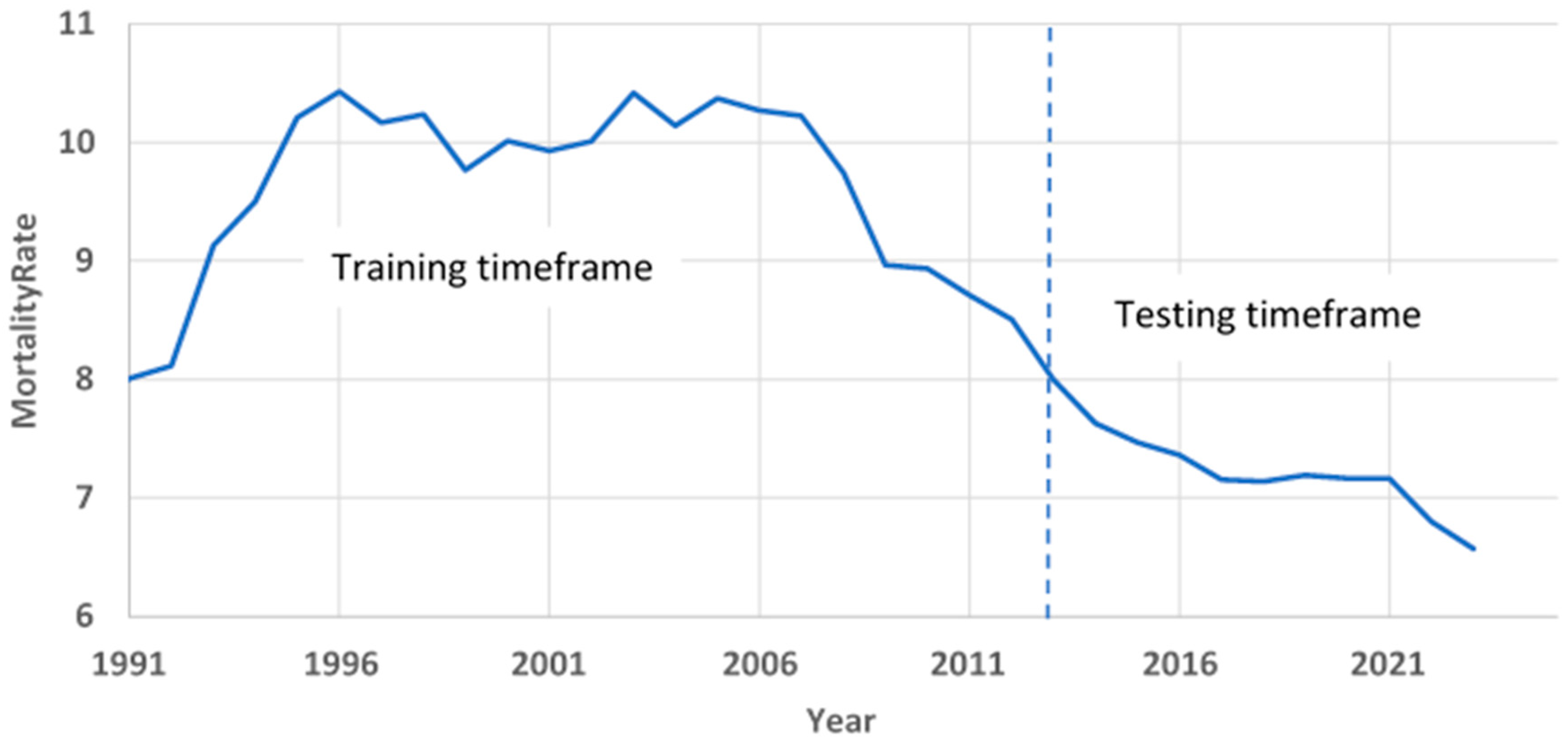
Figure 2.
Curves from the distant past are shown in yellow and the more recent curves are shown in purple.
Figure 2.
Curves from the distant past are shown in yellow and the more recent curves are shown in purple.
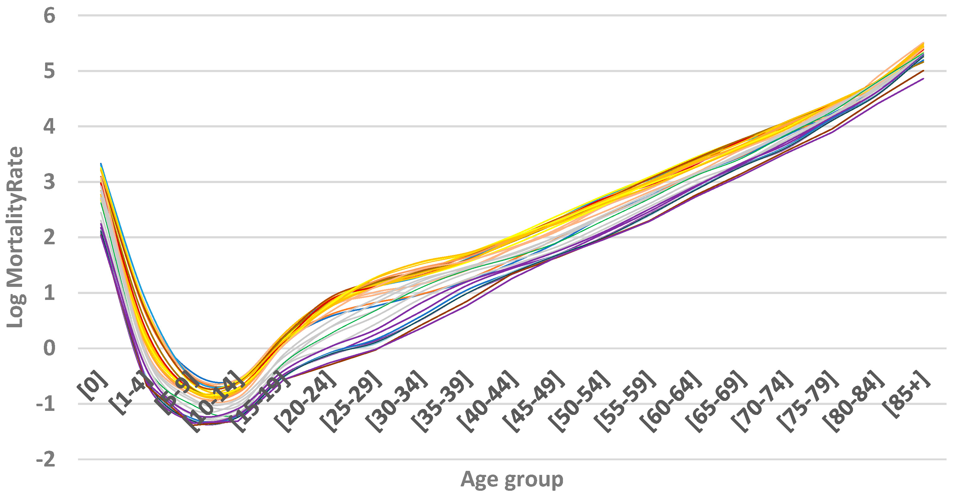
Figure 3.
LC model parameters.
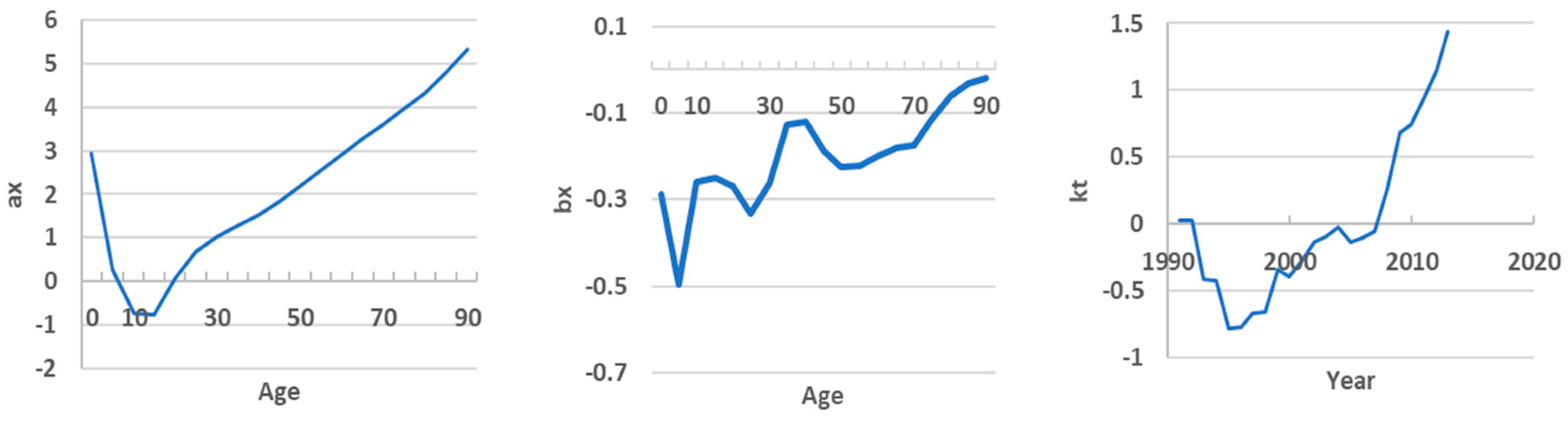
Figure 4.
Hyndman and Ullah model parameters.
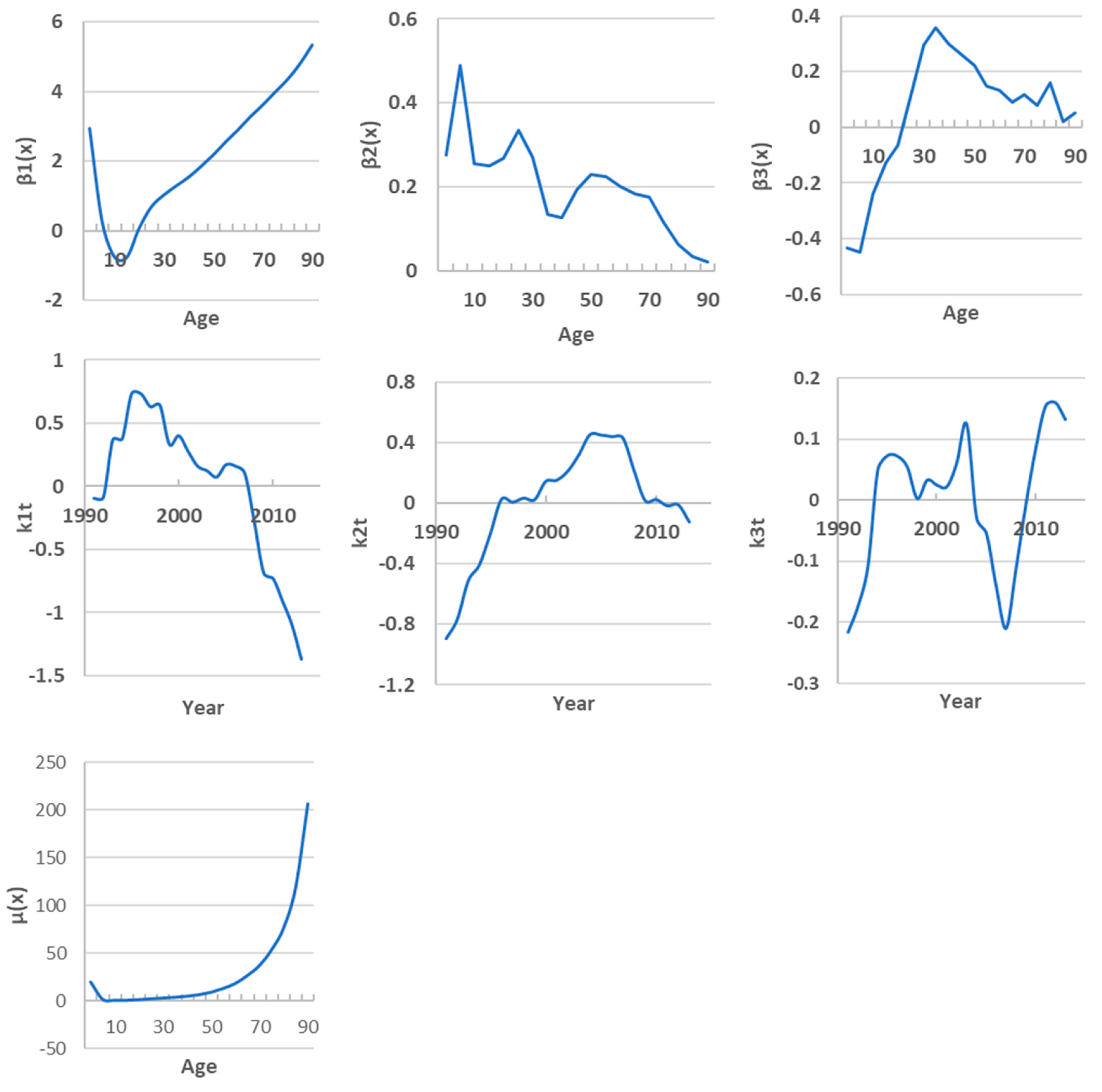
Figure 5.
Forecasting result. Orange line – score calculation on the training timeframe, blue line - forecasting without external factors, green line - forecasting with external factors, gray line – score calculation for the period 1991-2023.
Figure 5.
Forecasting result. Orange line – score calculation on the training timeframe, blue line - forecasting without external factors, green line - forecasting with external factors, gray line – score calculation for the period 1991-2023.
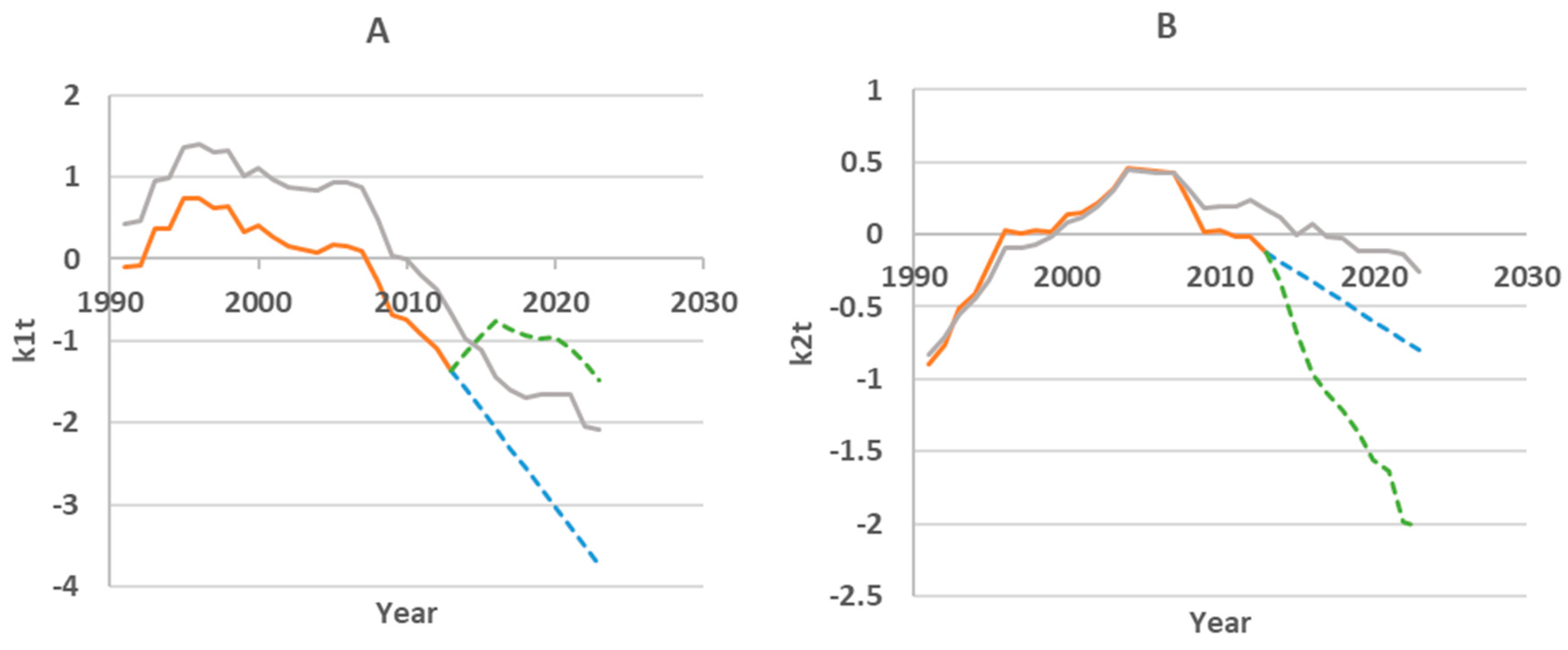
Figure 6.
Dynamics of external factors.
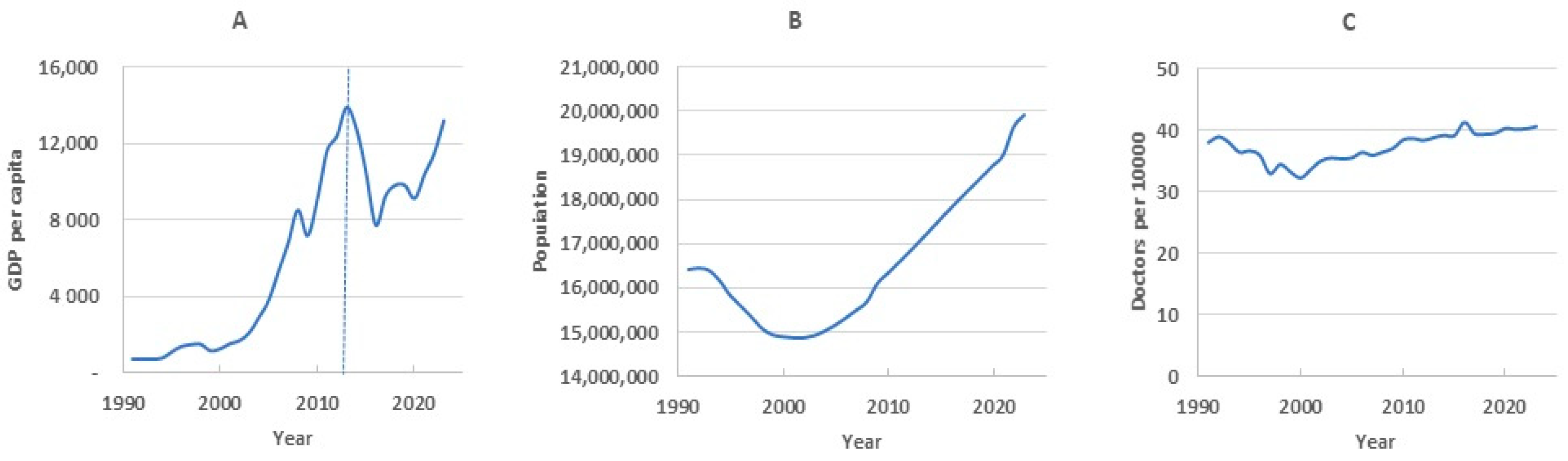
Figure 7.
Examples of long-term mortality trends in child (A) and adult (B) subpopulations.
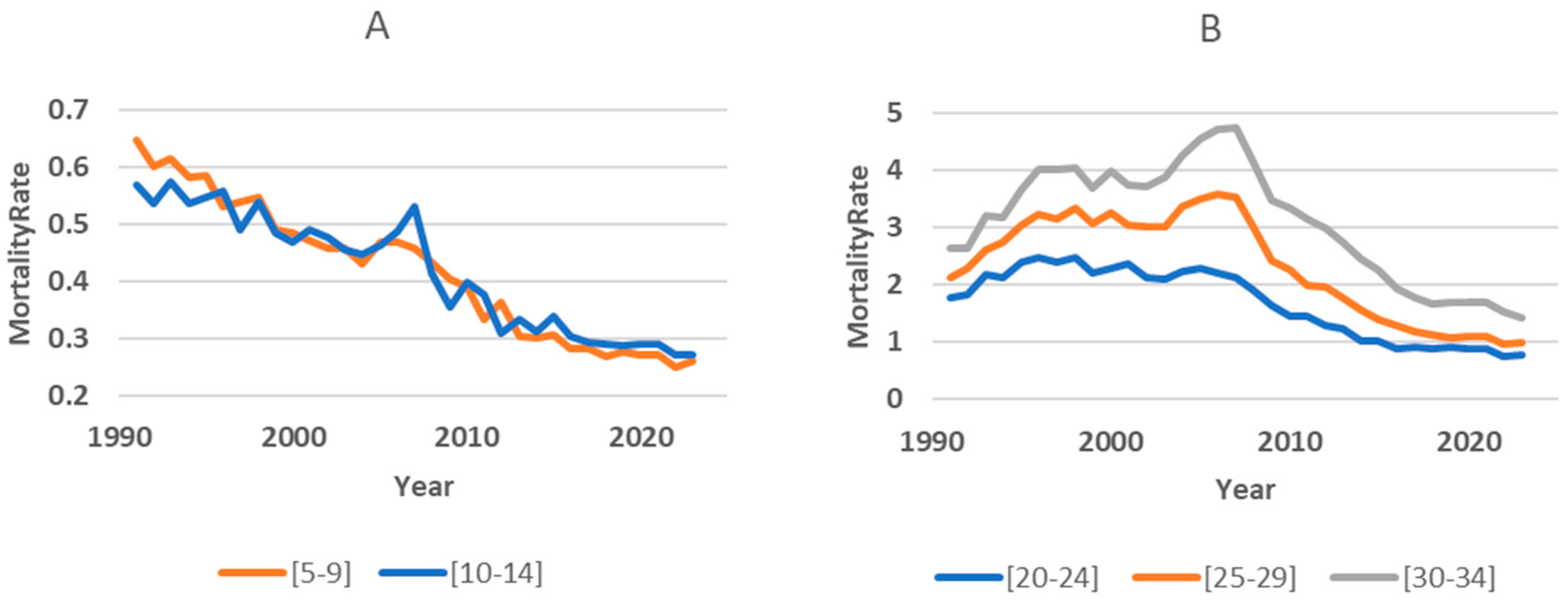
Figure 8.
Child subpopulation mortality forecasting results.
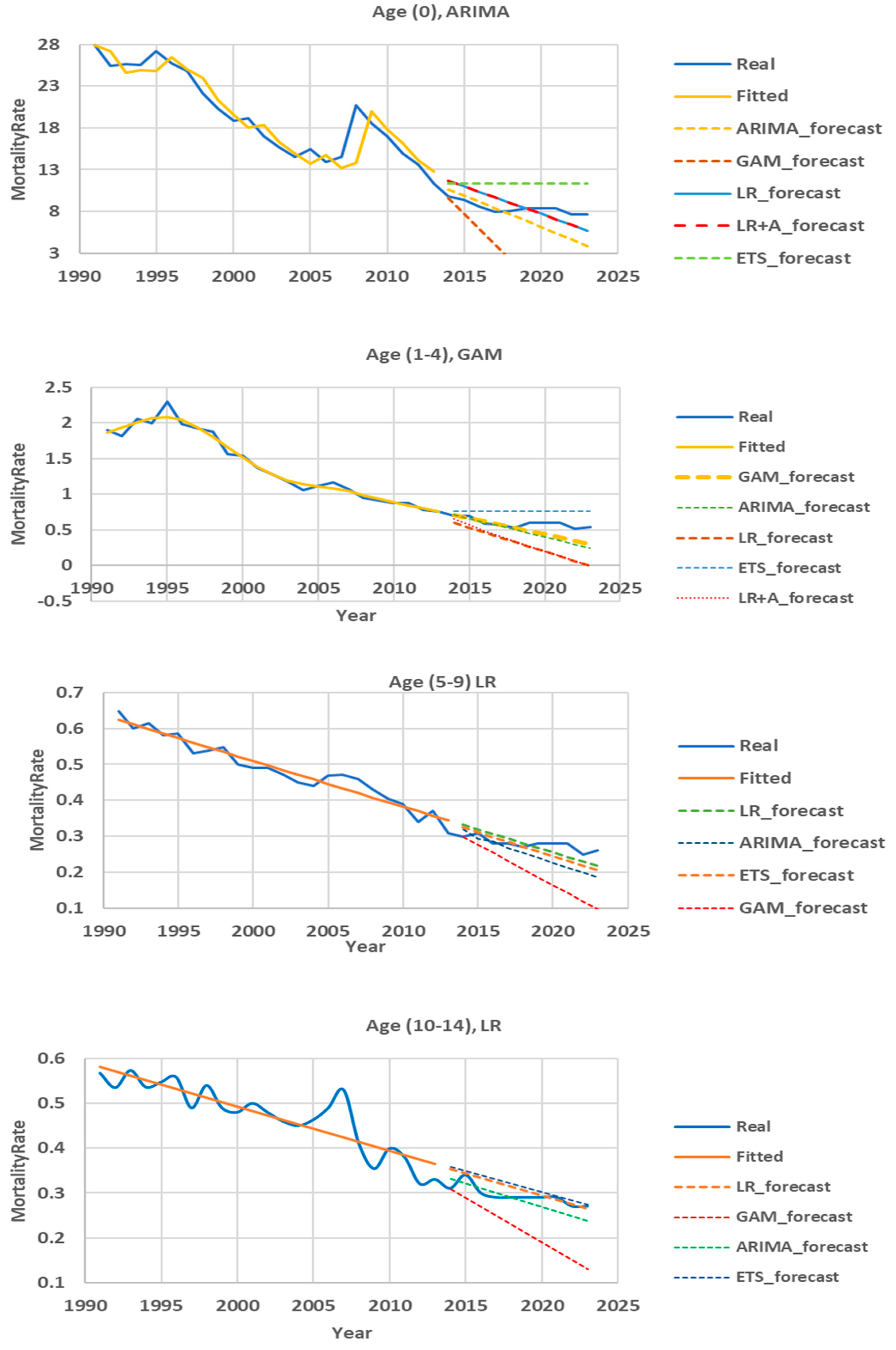
Figure 9.
Mortality forecasting up to 2033.
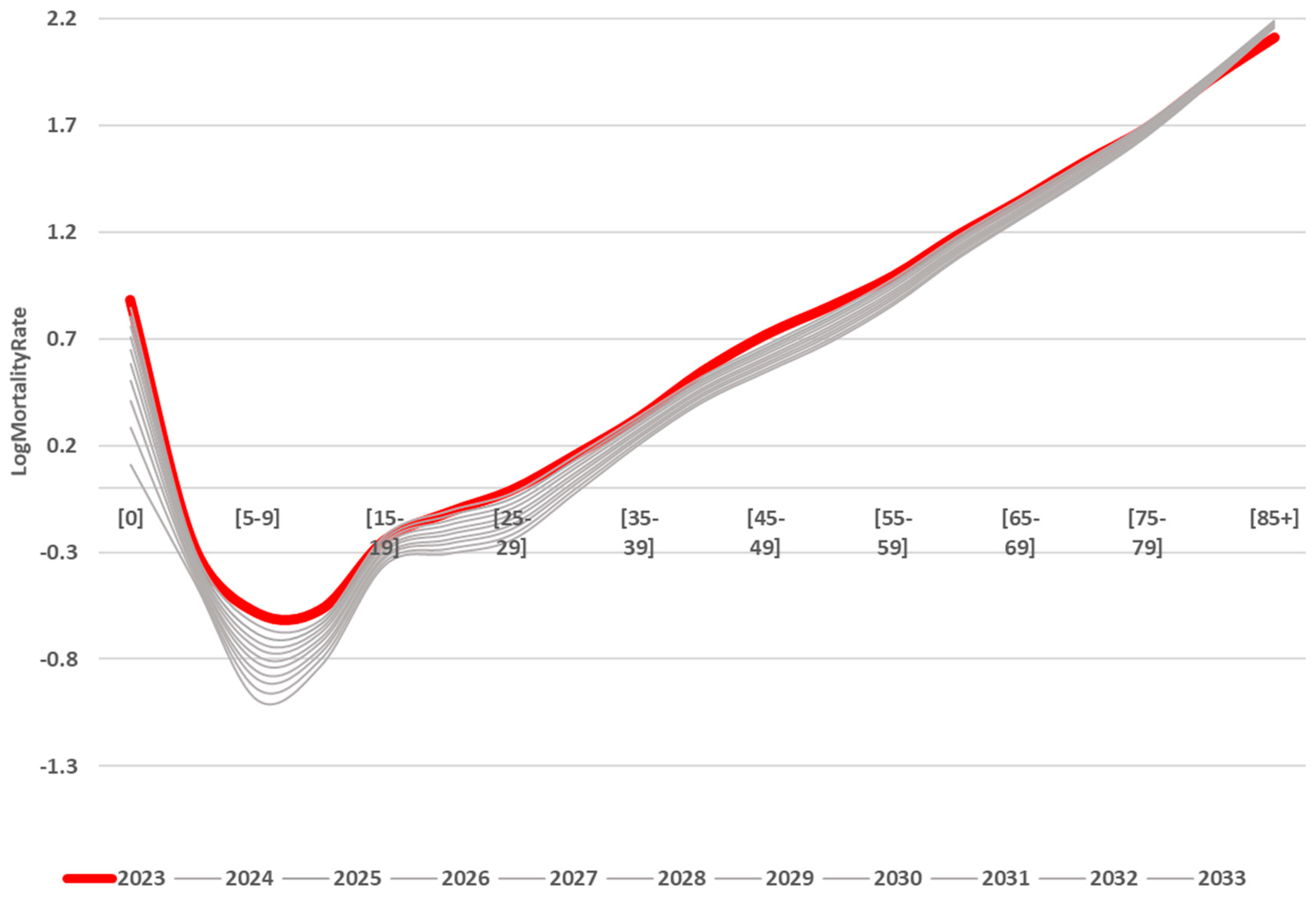

Table 1.
Lee-Carter model accuracy.
| Training timeframe | Testing timeframe | |
| Age group | MAPE, % | MAPE, % |
| 0 | 16.18 | 14.70 |
| 1-4 | 14.00 | 42.88 |
| 5-9 | 7.18 | 18.25 |
| 10-14 | 5.92 | 21.24 |
| 15-19 | 3.96 | 17.66 |
| 20-24 | 5.30 | 16.28 |
| 25-29 | 10.68 | 14.17 |
| 30-34 | 11.11 | 42.02 |
| 35-39 | 9.13 | 19.00 |
| 40-44 | 7.79 | 8.08 |
| 45-49 | 6.90 | 14.35 |
| 50-54 | 5.36 | 10.30 |
| 55-59 | 4.86 | 7.71 |
| 60-64 | 4.06 | 9.32 |
| 65-69 | 4.28 | 13.00 |
| 70-74 | 4.07 | 3.26 |
| 75-79 | 5.87 | 7.99 |
| 80-84 | 3.86 | 12.02 |
| 85+ | 6.84 | 8.02 |
| Mean | 7.23 | 15.80 |
Table 2.
Accuracy of Hyndman and Ullah model with different basis function types.
| Training timeframe (by default, B-splines, Fourier basis, Cubic splines) |
Testing timeframe (by default, B-splines, Fourier basis, Cubic splines) |
|
| Age group | MAPE, % | MAPE, % |
| 0 | 7.56 | 94.4 |
| 1-4 | 4.09 | 49.1 |
| 5-9 | 2.52 | 29.7 |
| 10-14 | 3.81 | 16.0 |
| 15-19 | 2.77 | 22.1 |
| 20-24 | 2.57 | 32.1 |
| 25-29 | 2.41 | 38.3 |
| 30-34 | 3.01 | 37.9 |
| 35-39 | 2.68 | 23.5 |
| 40-44 | 1.63 | 8.0 |
| 45-49 | 1.69 | 8.1 |
| 50-54 | 1.81 | 18.3 |
| 55-59 | 1.39 | 18.7 |
| 60-64 | 1.68 | 17.5 |
| 65-69 | 1.49 | 8.3 |
| 70-74 | 3.01 | 18.2 |
| 75-79 | 2.98 | 10.1 |
| 80-84 | 3.10 | 20.9 |
| 85+ | 5.70 | 13.4 |
| Mean | 2.94 | 25.5 |
Table 3.
Results of regression analysis.
| k1t (R2=0.84; F-statistic p-value = 6.69e-08) |
k2t (R2=0.89; F-statistic p-value = 1.34e-09) |
|||||
| Factor | γ | p-value | Contribution | γ | p-value | Contribution |
| Intercept | 3.707 | 0.008 | 8.256 | 2.48E-10 | ||
| GDP | -9.89E-05 | 5.97E-08 | 78.79% | 7.15E-05 | 7.15E-10 | 44.97% |
| Doctors | -0.112 | 0.04 | 20.83% | -0.011 | 0.7081 | 0.20% |
| Popul | 4.54E-08 | 0.782 | 0.38% | -5.23E-07 | 1.09E-05 | 54.83% |
Table 4.
Accuracy of Hyndman-Ullah model with regression of scores.
| Training | Testing without Exogenous Factors |
Testing with Exogenous Factors |
|
| Age group | MAPE, % | MAPE, % | MAPE, % |
| 0 | 7.56 | 94.4 | 78.69 |
| 1-4 | 4.09 | 49.1 | 50.90 |
| 5-9 | 2.52 | 29.7 | 30.15 |
| 10-14 | 3.81 | 16.0 | 21.18 |
| 15-19 | 2.77 | 22.1 | 19.10 |
| 20-24 | 2.57 | 32.1 | 29.80 |
| 25-29 | 2.41 | 38.3 | 35.50 |
| 30-34 | 3.01 | 37.9 | 36.26 |
| 35-39 | 2.68 | 23.5 | 23.56 |
| 40-44 | 1.63 | 8.0 | 9.20 |
| 45-49 | 1.69 | 8.1 | 9.53 |
| 50-54 | 1.81 | 18.3 | 21.08 |
| 55-59 | 1.39 | 18.7 | 19.83 |
| 60-64 | 1.68 | 17.5 | 19.22 |
| 65-69 | 1.49 | 8.3 | 7.03 |
| 70-74 | 3.01 | 18.2 | 18.01 |
| 75-79 | 2.98 | 10.1 | 10.55 |
| 80-84 | 3.10 | 20.9 | 18.75 |
| 85+ | 5.70 | 13.4 | 13.87 |
| Mean | 2.94 | 25.5 | 24.85 |
Table 5.
Accuracy of adult subpopulation mortality Hyndman and Ullah model.
| Training timeframe | Testing timeframe | |
| Age group | MAPE, % | MAPE, % |
| 15-19 | 3.46 | 6.77 |
| 20-24 | 1.70 | 12.88 |
| 25-29 | 2.57 | 9.65 |
| 30-34 | 2.14 | 17.20 |
| 35-39 | 1.89 | 4.68 |
| 40-44 | 1.57 | 14.53 |
| 45-49 | 1.61 | 17.25 |
| 50-54 | 1.69 | 10.00 |
| 55-59 | 1.50 | 7.32 |
| 60-64 | 1.46 | 7.13 |
| 65-69 | 1.57 | 12.41 |
| 70-74 | 2.30 | 3.39 |
| 75-79 | 2.70 | 3.16 |
| 80-84 | 3.01 | 13.69 |
| 85+ | 5.25 | 7.68 |
| Mean | 2.29 | 9.85 |
Table 6.
Mortality prediction accuracy of different models for age group (0).
| APE, % | |||||
| Year | ARIMA | ETS | GAM | LR | LR+A |
| 2014 | 8.22 | 15.87 | 2.58 | 18.52 | 12.42 |
| 2015 | 5.07 | 21.04 | 17.91 | 16.80 | 12.65 |
| 2016 | 6.35 | 32.60 | 31.63 | 20.27 | 17.31 |
| 2017 | 5.72 | 43.63 | 49.29 | 21.97 | 19.87 |
| 2018 | 4.96 | 41.85 | 72.98 | 12.23 | 10.88 |
| 2019 | 17.80 | 36.08 | 96.20 | 0.20 | 1.05 |
| 2020 | 26.78 | 36.08 | 118.33 | 8.08 | 8.63 |
| 2021 | 35.76 | 36.08 | 140.45 | 15.96 | 16.32 |
| 2022 | 39.78 | 48.31 | 168.20 | 17.00 | 17.26 |
| 2023 | 49.23 | 49.28 | 192.92 | 25.10 | 25.27 |
| Mean | 19.97 | 36.08 | 89.05 | 15.61 | 14.17 |
Table 7.
Mortality prediction accuracy of different models for 1-4 age.
| APE, % | |||||
| Year | ARIMA | ETS | GAM | LR | LR+A |
| 2014 | 1.19 | 8.57 | 1.23 | 14.53 | 6.36 |
| 2015 | 6.19 | 8.57 | 5.23 | 24.14 | 19.19 |
| 2016 | 4.31 | 31.03 | 6.59 | 20.04 | 16.42 |
| 2017 | 2.92 | 33.33 | 0.53 | 30.44 | 28.21 |
| 2018 | 5.35 | 43.40 | 0.40 | 37.88 | 36.43 |
| 2019 | 25.00 | 26.67 | 19.55 | 56.34 | 55.56 |
| 2020 | 33.61 | 26.67 | 27.08 | 67.55 | 67.08 |
| 2021 | 42.22 | 26.67 | 34.62 | 78.76 | 78.48 |
| 2022 | 42.16 | 49.02 | 31.94 | 88.20 | 88.00 |
| 2023 | 54.94 | 40.74 | 44.09 | 101.31 | 101.20 |
| Mean | 21.79 | 29.47 | 17.13 | 51.92 | 49.69 |
Table 8.
Mortality prediction accuracy of different models for 5-9 age.
| APE, % | |||||
| Year | ARIMA | ETS | GAM | LR | LR+A |
| 2014 | 6.77 | 8.17 | 0.30 | 10.56 | 10.56 |
| 2015 | 5.41 | 0.41 | 10.75 | 2.90 | 2.90 |
| 2016 | 2.15 | 6.43 | 9.19 | 9.39 | 9.39 |
| 2017 | 4.19 | 1.70 | 17.20 | 4.86 | 4.86 |
| 2018 | 5.14 | 0.57 | 22.44 | 4.04 | 4.04 |
| 2019 | 13.94 | 7.76 | 33.21 | 4.20 | 4.20 |
| 2020 | 18.78 | 12.49 | 41.22 | 8.74 | 8.74 |
| 2021 | 23.92 | 17.22 | 49.22 | 13.27 | 13.27 |
| 2022 | 20.37 | 12.58 | 52.10 | 7.94 | 7.94 |
| 2023 | 28.88 | 21.04 | 62.56 | 16.36 | 16.36 |
| Mean | 12.96 | 8.83 | 29.82 | 8.23 | 8.23 |
Table 9.
Mortality prediction accuracy of different models for 10-14 age.
| APE, % | |||||
| Year | ARIMA | ETS | GAM | LR | LR+A |
| 2014 | 7.03 | 15.85 | 0.28 | 14.29 | 14.29 |
| 2015 | 5.49 | 2.82 | 14.91 | 1.29 | 1.29 |
| 2016 | 3.63 | 13.35 | 10.19 | 11.49 | 11.49 |
| 2017 | 3.60 | 13.96 | 13.94 | 11.92 | 11.92 |
| 2018 | 0.00 | 10.66 | 20.79 | 8.50 | 8.50 |
| 2019 | 3.60 | 7.37 | 27.63 | 5.08 | 5.08 |
| 2020 | 7.20 | 4.07 | 34.48 | 1.66 | 1.66 |
| 2021 | 10.80 | 0.78 | 41.33 | 1.76 | 1.76 |
| 2022 | 8.07 | 4.71 | 44.34 | 1.85 | 1.85 |
| 2023 | 11.93 | 1.17 | 51.69 | 1.82 | 1.82 |
| Mean | 6.14 | 7.47 | 25.96 | 5.96 | 5.96 |
Disclaimer/Publisher’s Note: The statements, opinions and data contained in all publications are solely those of the individual author(s) and contributor(s) and not of MDPI and/or the editor(s). MDPI and/or the editor(s) disclaim responsibility for any injury to people or property resulting from any ideas, methods, instructions or products referred to in the content. |
© 2024 by the authors. Licensee MDPI, Basel, Switzerland. This article is an open access article distributed under the terms and conditions of the Creative Commons Attribution (CC BY) license (http://creativecommons.org/licenses/by/4.0/).
Copyright: This open access article is published under a Creative Commons CC BY 4.0 license, which permit the free download, distribution, and reuse, provided that the author and preprint are cited in any reuse.


