

Submitted:
23 December 2024
Posted:
25 December 2024
You are already at the latest version
Abstract
In the world of evolution equations, higher dimensional nonlinear partial differential equation has attracted a vast attention for investigation due to the fact that, it models various interesting physical phenomena existent in, fluids dynamics (theoretical physics), other nonlinear sciences and engineering. In the wake of this, analytical examination of a nonlinear generalized Ablowitz-Kaup-Newell-Segur water wave equation arising from theoretical physics is the given consideration in this article. Leveraging on the robust Lie group theoretic approach, applied to differential equations, one investigates the understudy equation in a detailed form with a view to securing various results of interest. Thus, in executing these, one first computes a seven-dimensional Lie algebra L7 associated to the nonlinear generalized Ablowitz-Kaup-Newell-Segur water wave equation in a stepwise structure. Sequel to this, one parameter groups of transformation associated to L7, is studied. Additionally, commutation relations and adjoint representations of the Lie algebra are tabularly explicated. A detailed computation of a one dimensional optimal system associated to L7 is furnished. Thereafter, various obtained sub-algebras are invoked in effectuating reductions of the model under examination to ordinary differential equations, so that diverse pertinent exact solutions are attained. The success in this regard entrenched solutions like trigonometric, exponential, logarithmic and hyperbolic functions. Besides, algebraic solutions among which arbitrary functions exist and quadrature are found. Sound knowledge of these results are further engendered by numerically simulating them. Wave structures of diverse interests are achieved. Furthermore, conservation laws of the equation are calculated via conserved vectors theorem by Ibragimov using the related formal Lagrangian to the model.
Keywords:
generalized multi-dimensional Ablowitz-Kaup-Newell-Segur water wave equation
; Lie group theory
; invariant analysis: analytic solutions
; conserved vectors
1. Introduction
Nonlinear partial differential equations (NLNPDEEs) play a significant role in various fields such as applied mathematics, physics, and engineering. These equations are essential for modeling physical phenomena and have numerous practical applications. However, solving NLNPDEEs can be challenging due to the lack of systematic methods for finding analytic solutions, unlike linear partial differential equations (LNPDEEs). Despite the importance of finding analytic solutions for NLNPDEEs, there remains a need for new techniques to discover these solutions efficiently. The exploration of nonlinear wave phenomena has had a significant impact on various natural sciences such as biology, mathematics, and several branches of physics including condensed matter physics, nonlinear optics, chemical physics, plasma physics, solid-state physics, and fluid dynamics. The analysis of nonlinear partial differential equations is a thriving and dynamic area of study in theoretical physics, applied mathematics, and various engineering disciplines. Researchers are particularly interested in discovering exact solutions for traveling waves in these differential equations that describe important physical and dynamic processes [1–16]. However, in recent times, numerous researchers have focused on creating effective methods to analyze solutions of the Nonlinear Nonlocal Partial Differential Equations. Some of these techniques consist of: Kudryashov’s approach [17], simplest equation technique [18], sine-Gordon equation expansion technique [19], Hirota’s bilinear approach [20], -expansion technique [21], power series solution technique [22], Darboux transformation approach [23], and among others. Additional, techniques such as Painlevé expansion technique [24], bifurcation approach [25], homotopy perturbation [26], extended homoclinic test technique [27], tanh-coth technique [28], Adomian decomposition technique [29], Symmetry group analysis [30,31], F-expansion approach [32], Bäcklund transformation method[33], extended simplest equation technique [17], Cole-Hopf transformation approach [34], rational expansion approach [35], and many more have been developed. Since the establishment of Kadomtsev and Petviashvili’s hierarchy of equations over fifty years ago, numerous research papers have been published, each delving into different aspects of this complex field of equations. For instance, see [36,37,38,39,40,41,42], one mentions but a few here.
Sophus Lie, a prominent Norwegian mathematician, revolutionized the study of Lie symmetries from 1842 to 1899. Lie discovered that the seemingly random methods used to solve ordinary differential equations (ODEEs) could be organized into a structured theory based on the consistency of differential equations within a continuous symmetry group. By applying invariant solutions to a symmetry group derived from a partial differential equation (PDE), one can determine a solution to the differential equation (DE) with fewer independent variables. Among these solutions are similarity solutions, traveling wave solutions, and other closed-form solutions that hold significance in the physical world [30,31].
Exploration of differential equations has revealed numerous valuable applications of conserved quantities. One such application is the ability to determine the integrability of a chosen partial differential equation, providing a deeper insight into its properties. Utilizing conserved quantities can also ensure the existence and uniqueness of solutions to a differential equation. Furthermore, these quantities play a crucial role in validating numerical solution methods. Despite these benefits, a challenge lies in identifying the conserved quantities relevant to a specific differential equation. The general multiplier method offers a systematic approach to discovering conserved quantities for differential equations, whether or not they are based on variational principles [43,44,45,46,47,48,49].
A (2+1)-dimensional AKNS equation given as [50]
with constant coefficient which indicated the dissipative characteristic effects of the system was investigated in [50] whereby the authors engaged the idea of Hirota’s bilinear approach to seeking for the closed-form solution of equation (1). This technique made it possible to procure multiple singular closed-form soliton solutions of the equation. The researchers in [51] through the involvement of Bilinear Bäcklund transformation explicitly established some wave solutions founded on a multidimensional Riemann theta function which are periodic. Wazwaz [52] utilized the simplified Hirota’s bilinear approach developed by Hereman [53] to find multiple-soliton solutions of equation (1). In [54], some exact travelling wave solutions of equation (1) were gotten for the (2+1)-dimensional AKNS equation by utilizing the improved tanh method. Authors in [55] applied binary Bell polynomials to secure bilinear Bäcklund transformation, the bilinear representation, conservation laws as well as the Lax pair of the equation (1). When , equation (1) converts to the (2+1)-dimensional AKNS equation which is closely interrelated with the Schwarz KdV equation through the use of a Miura transform [54,56]. Mothibi in [57] considered the generalized version of (1) and then generated the conservation laws of the equation via Noether theorem. Hiu et al. [58] employed the truncated Painlevè expansion together with consistent Riccati expansion abbreviated as "CRE" to gain soliton-cnoidal wave interaction solutions of equation (1) explicitly. The divers closed-form solutions of AKNS equations (1) are procured by virtue of extended homoclinic, tanh function method as well as symmetry analysis [54,56,59,60].
The Ablowitz-Kaup-Newell-Segur (AKNS) system [61]
whereby the subscripts stands for the partial derivatives. We also have functions and depending on x and t. AKNS system (2) is one of the members of the family of AKNS models. In [62] the researchers dissolved the AKNS system (2) to integrable Hamiltonian systems that are finitely-dimensional via Bargmann adjoint symmetry constraints. Moreover, in [63], one-parameter groups of solutions of the single non-linear Schrödinger equation which is regarded as a special reduction type of AKNS (2) was presented through the engagement of Lie symmetry technique. Li et al. [64] got some multisoliton solutions of system (2) by utilizing Darboux transformation. In the same vein, Wang et al. in [65] procured some new solutions which are multisoliton. Furthermore, the authors in [64,65] transformed AKNS system (2) into the (1+1)-dimensional integrable non-linear dispersive-wave system
via the engagement of the transformation
The fourth-order nonlinear (2+1)-dimensional Ablowitz-Kaup-Newell-Segur water equation (AKNS) [66]
with a perturbation parameter , is an important partial differential equation which has numerous applications in various fields of study including physics together with some other nonlinear sciences. In [66], Asghar et al. adopted simple equation approach as well as its modified form to analytically secure travelling wave solutions to the earlier-mentioned AKNS equation (3). Helal et al. [67], conducted stability analysis on AKNS equations (3) whereby extended auxiliary equation method was involved to gain new soliton-like solutions for the underlying equation. Besides, they got symmetrical solution, non-symmetrical kink solution, bell-shaped solitary wave solution, solitary wave solution as well as travelling wave solution. The algorithmic scheme of -expansion technique was engaged in the construction of new solutions for AKNS (3) in [68]. Authors in [69] made a description of a unified scheme for all equations of AKNS hierarchy as well as their combinations. In furtherance to that, they presented examples of solutions that fulfilled different equations for various parameters by precisely taking into consideration a rank-2 quasi- rational solution which can as well be employed in examining divers integrable models featuring in nonlinear optics.
In this study, we investigate the (2+1)-dimensional generalized Ablowitz-Kaup-Newell-Segur equation (2D-gnrAKNSe)
where , and are real-valued constants. It is noteworthy to state here that, we obtained the generalized AKNS (4) by taking and in equation (3). Explicit analysis of 2D-gnrAKNSe (4) is effectuated in this article as follows; Introduction is explicated in section 1, whereas the essential method of solution (Lie group theory) is implemented in calculating the point symmetries that constitute the Lie algebra of the model (2D-gnrAKNSe (4)) in Section 2. Additionally, groups of transformations in one parametric format is computed. In tabular form, commutation relations as well as adjoint representation of the computed Lie algebra are expressed. Moreover, the subalgebras found are engaged in discharging symmetry reductions of (4) to various ordinary differential equations (ODEE). Thereafter, wave dynamics of the solutions are put into consideration via numerical simulation of the results, in section 3. Thereafter, conservation laws of the considered model (4) are calculated by utilizing the Ibragimov’s theorem for conserved vectors. These are presented in section 4. Finally, at the end, concluding remarks are given in section 5.
2. Lie Point Symmetry Analysis
This section of the article calculates and presents the Lie point symmetries of 2D-gnrAKNSe (4) and thereafter engages them to find exact solutions.
2.1. Determination of Lie point symmetries of (4)
The Lie group of transformation is defined as
The group of symmetries of 2D-gnrAKNSe (4) will be calculated by contemplating a vector field given as
with and taken as functions depending on t, x, y and u, secures a Lie point symmetry of 2D-gnrAKNSe (4) if the invariant condition
holds whenever . Precisely Pr denotes the third prolongation of which is expressed in the form
with the coefficients , , , , , , , , given respectively as
and the total derivatives are stated as
For the main purpose of determining Lie group (5) admitted by 2D-gnrAKNSe (4), we invoke (8) into criteria (7). We make the coefficients of varying derivatives order of u equal to zero. Thus, gaining overdetermined systems of LNPDEEs with respect to functions , , , and , viz;
The solution to system (10) secured via computer software furnishes us with the values of coefficient functions expressed as
Assuming that arbitrary function , then we achieve Lie point symmetries presented as
2.2. One-parameter Lie group transformation using
This subsection furnishes the one-parameter transformation group of 2D-gnrAKNSe (4) using . In order to gain the transformation group generated by generators (12), its integral curves are needed to be secured. Thus, we come by the theorem:
Theorem 2.2.
If group constitutes the one parameter group generated by vectors in (12), then, for each of the vectors with any small positive number ϵ, we have accordingly
Theorem 2.3.
In consequence of Theorem 2.2, we can say that if satisfies the 2D-gnrAKNSe (4), so also are the functions established as
where is any positive number.
Remark 2.1.
In general, it is noteworthy to declare here that to each one-parameter subgroups of the full symmetry group system, there will be an associated family of solutions referred to as group-invariant solutions.
2.3. Optimal system of sub-algebras
It is well understood that the Lie group theoretic approach performs a crucial function in securing exact solutions of differential equations together with the performance of symmetry reductions. Having identified the fact that any linear combination of infinitesimal generators is also an infinitesimal generator, there are absolutely infinitely many different symmetry subgroups which basically occasions varying types of solutions. This in turn is significant and also necessary for one to have a complete understanding of the involved invariant solutions. Besides, it is sufficient to seek invariant solutions that are not analogous by transformations in the full symmetry group, since any transformation in the full symmetry group maps a solution to another solution. This has consequently led to the concept of an optimal system [70]. The task involved in obtaining an optimal system of subalgebras is as well equivalent to that of achieving an optimal system of subgroups. This classification problem for one-dimensional subalgebras is fundamentally same as the problem involved in the classification of the orbits of adjoint representation. Thus, this problem is thrashed via the engagement of naive approach whereby a general element taken from the Lie algebra is subjected to different adjoint transformations so that it can be simplified as much as possible. It was due to [70,71] that the idea of imploring adjoint representation to classify group-invariant solution was conceived. We define the Lie series as
which include the adjoint representation[31] with regarded as group parameter together with defined as the Lie algebra commutator (Lie bracket) and . Thus we construct the commutator table using the relation in Table 1.
Table 1. Commutator table of the Lie algebra of 2D-gnrAKNSe (4)
| 0 | 0 | 0 | 0 | 0 | ||||
| 0 | 0 | 0 | 0 | 0 | 0 | 0 | ||
| 0 | 0 | 0 | 0 | 0 | ||||
| 0 | 0 | 0 | 0 | 0 | ||||
| 0 | 0 | 0 | 0 | |||||
| 0 | 0 | 0 | 0 | |||||
| 0 | 0 | 0 |
The real function is commonly referred to as an invariant which satisfies the relation for all with any subgroup g. Moreover, is invariant if and only if one can compute the values of , for and so we have
Solving the system of equations secured in (14), we achieve the value of invariant as
where G represents an arbitrary function dependent on , and .
Now, we can anticipate the simplification of a given arbitrary element
of the 2D-gnrAKNSe (4) Lie algebra represented as . We notice at this junction that we can represent elements of via vector since each of the elements can be expressed in the structure of (16) for some constants . As a result, the adjoint action can be taken in this regard as a group of linear transformations of vector .
Table 2. Adjoint table of Lie algebra for seven parameters.
where .
Thus, an adjoint action is contemplated for Lie algebra and so by imploring Table 2, we can conveniently consider the theorem:
Theorem 2.4.
The one-dimensional subalgebras optimal system for 2D-gnrAKNSe (4) Lie algebrais presented as
(i) 1 :
(ii) 2 :
(iii) 3 :
(iv) 4 :
(v) 5 :
(vi) 6 :
(vii) 7 :
(viii) 8 : .
Proof. A function : ↦ defined by is a linear map, for . Furthermore, the matrix of the function , with regards to the basis are given as:
Now, suppose we let
where matrix A is defined as the universal matrix calculated and presented as
Let be an element in the Lie algebra. The application of the most general adjoint action to where and can be revealed to be equivalent, can be shown with respect to with the relation
with A standing for the universal adjoint matrix. We now add a remark here:
Remark 2.2.
We notice that once equation (18) has a solution, then and Y as defined are equivalent under the adjoint action.
Therefore, transforms this way:
Now, the construction of one dimensional subalgebra optimal system of 2D-gnrAKNSe (4) can be performed. We contemplate the invariant function G depending on its sign[31,72] and so we do these cases, viz:
Case 1. , , ,
Imploring the selection of parameters as , as well as in adjoint equation (18), we secured a solution
Therefore, we gain the optimal representative .
Case 2. ,
This case, dependent on the value of the constant parameters occasions four subcases. We highlight these subcases in the subsequent part of the study.
Case 2.1., , ,
We insert the parametric values , alongside in system (18), then we get
So, we select the optimal representative .
Case 2.2., , ,
Moreover, we invoke the parametric values of as , alongside in adjoint system (18), we achieve the solution
In consequence, we select the optimal representative .
Case 2.3., , ,
We further substitute parameters in adjoint system (18) as , alongside and obtain solutions with regards to , , and as
Hence, we select the optimal representative .
Case 2.4., , ,
In this subcase, we insert the values , and in the system of partial differential equations (14), we gain a new invariant solution as
We proceed to consider two major cases of the new invariants as and and explore them.
Case 2.4.1., , ,
We observe that if , then we can say and so without loss of generality, we can choose parametric values of as , along with in adjoint system (18). Thus, we secure the solution
Therefore, we choose the optimal representative . Now, for invariant , we contemplate three possible options.
Case 2.4.2., , ,
In the first place, we contemplate , , and by substituting the appropriate values of parameters , that is, , along with , in system (18), one obtains
Thus, we select the optimal representative . In addition, if we choose , together with , in system (18), one then gets
Thus, we select the optimal representative .
Case 2.4.3., , ,
Now, we consider , , and insert the values of parameters , along with , in adjoint system (18), we gain
In consequence, we choose the optimal representative . Besides, if we choose , together with , in system (18), we then achieve the result
As a result, we select the optimal representative . Finally if we contemplate , , , make proper choice of and substitute them in (18) as we have earlier done, then we achieve the solution
Therefore, we select the optimal representative . Now, based on the outcome of our computations, we achieve eight members of the one-dimensional subalgebras optimal system for 2D-gnrAKNSe (4) as: , , , , , , and , for all . This ends the proof of the theorem.
2.4. Lie Group-Invariants and Similarity Solutions of (4)
This section furnishes the utilization of the obtained optimal system of subalgebras explicated earlier in reducing 2D-gnrAKNSe (4) to ordinary differential equations and subsequently obtaining possible exact solutions of the model. In achieving this, we take into account the relation purveys as
which is often referred to as the characteristic equations or Lagrangian system.
2.4.1. Invariant Solutions Using Subalgebra Component
In the first place, we contemplate time translation symmetry which when apply (29) engenders invariants and with group invariant . Inserting the function in equation (4) gives the NLNPDEE
Thus, we have the solution to 2D-gnrAKNSe (4) in this regard as
where and are arbitrary constants. Further exploration of (30) gives
In utilizing the computed symmetries to reduce (4), we first contemplate which gives , where . Thus, we use the function and secure which when solved leads to a solution of 2D-gnrAKNSe (4) as
with integration constants and . Meanwhile, gives a trivial solution of (4). We now explore and achieve , reducing (4) to
which is a trigonometric solution of 2D-gnrAKNSe (4), where are arbitrary constants. Exploring leads to , where leading to linear ordinary differential equation (LNODE) just like the case of , and giving
with arbitrary integration constants and . Now, we take on , since purveys a trivial solution of model (4) and so it gives , where we have . Substituting the obtained function in (4) secures
Next, we contemplate and on solving the associated system (29) leads to
where . Inserting the relation in (36) into (4) gives LNODE as we have in the case of which solves to secure a solution of 2D-gnrAKNSe (4) here as
where and are arbitrary integration constants. Finally, under , we engage symmetry operator which yields the invariant expressed here as
2.4.2. Invariant Solutions Using Subalgebra Component
Now, we take on the second member of the achieved-optimal system which is . Solving the related Lagrangian system purveys an invariant explicated as
Utilizing the gained-function transforms (4) to a NLNPDEE furnished as
Here, we secure a solution of model (4) in this instance as
where arbitrary functions and are depending on their respective arguments. Further exploration of the gained NLNPDEE (42) reveals the four symmetries, viz
Using symmetry operator furnishes a trivial solution of (4) and so in the case of one secures , where we have which reduces (4) to
Hence, we gain a trigonometry solution of (4) in this case as
with arbitrary constants , and . In the case of symmetry generator , one gains , where we have . Thus, we have (4) become
In addition, for , one achieves , where , so (4) becomes
2.4.3. Invariant Solutions Using Subalgebra Component
The associated characteristic equation to solves to give the function , where , . Using these reduce (4) to
In this case, we have a solution of (48) in this regard as the tan-hyperbolic function
with arbitrary constants and . Besides, (48) furnishes symmetries
In order to attain interesting results, we let . So, applying Lie theoretic approach to , one achieves , where we have . Thus, substituting the function in (48) further reduces it to
2.4.4. Invariant Solutions Using Subalgebra Component
In the case of subalgebra , we calculate its invariants and so have
On applying the calculated-invariants in (4), one attains NLNPDEE
Consequently, we secure a solution of model (4) in this regard as
where we have arbitrary functions and depending on their arguments. Here, (53) admits three symmetries , , and . Having found out that and give trivial solutions of (4), we then explore and achieve , where we have . This further transforms (4) to
2.4.5. Invariant Solutions Using Subalgebra Component
Here, we take a look at and by following the usual steps secures; , where and . Invoking these in (4) gives NLNPDEE
Exploring (56) further via Lie symmetry approach leads to the attainment of
In case of , we have invariant , where , reducing (4) to
2.4.6. Invariant Solutions Using Subalgebra Component
Exploring , we have a group invariant relation obtained as , where as well as . Inserting the function in (4) produces
2.4.7. Invariant Solutions Using Subalgebra Component
Investigation of from the Lie symmetry analysis standpoint purveys
Invoking the function in (4) gives a fourth order NLNPDEE explicated as
Hence, in this regard, we gain a solution of 2D-gnrAKNSe (4) as
where we have arbitrary constants and . In addition, (61) admits
Considering , one obtains , where . Introducing the obtained function transforms 2D-gnrAKNSe (4) further into the NLNODE
2.4.8. Invariant Solutions Using Subalgebra Component
We study the sublagebra component which has the invariant
On inserting the function in (4), one secures the equation
Further analysis carried out on (66) revealed that it admits
3. Graphical Appraisal of Solutions and Discussion
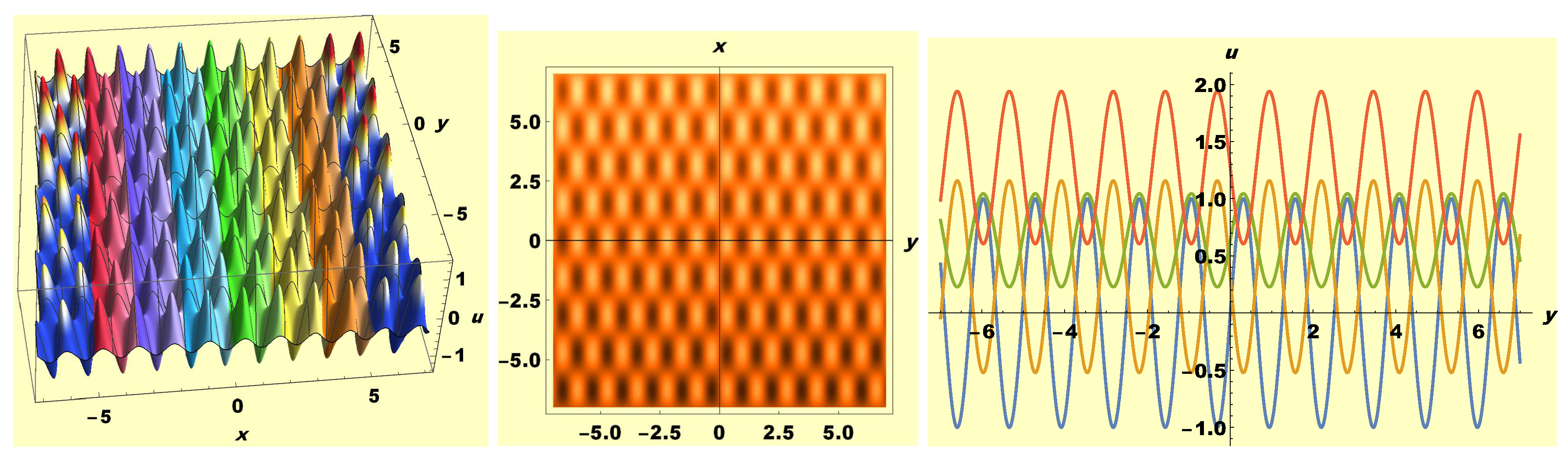
The notion of presenting the streaming nature of wave motions that depicts the physcial meaning exhibited by exact solutions to differential equation (DE) is of a great essence. This is due to the fact that the phenomena represented by the model that the DEs portray can only be better understood and then appreciated when their solutions are pictorially enhanced. In view of these, this section exhibits various wave structures represented by some of the obtained exact solutions to 2D-gnrAKNSe (4). The graphs are given in form of three dimensional (3-D), two dimensional (2-D) and density plots through the utilization of suitable choice of parameters. Now, in order to copiously view the interesting wave structures depicted by the exact periodic solution obtained in (33) which contains variables t and x ( ), pictorial demonstration of the result is given in Figure 1, Figure 2, Figure 3 and Figure 4. Thus, the trigonometry solution is first plotted in Figure 1 by selecting the parameter values as; , , , , , , , where interval exits. In addition, Figure 2 also delineates the wave motion of the solution by doing , , , , , , , with variable interval . In similar way, Figure 3 is plotted with the data set; , , , , , , , in the interval . In the case of Figure 4, one adopts the selection of parameter values , , , , , , , where one has . Another solution to be graphically examined is the logarithmic-trigonometric solution (45) which is presented in Figure 5, Figure 6 and Figure 7. In the first place, the log-trigonometric function (45) is plotted as 3-D, 2-D and density graphs in Figure 5 using the unalike constant values , , , , , , , , where variable as well as . Similarly, one plots graphs in Figure 6 using the values , , , , , , , , with , where . In the case of Figure 7 the variant data set utilized are , , , , , , , , where one takes, alongside . The next three Figures depict the wave motion of tangent hyperbolic solution (49), Therefore, plotting graphs in Figure 8, the dissimilar parameter values invoked are , , , , , , , , at as well as . Likewise, in Figure 9, the kink wave structure is plotted using the data set , , , , , , , , where variable with . Regarding Figure 10 in 3-D, 2-D and density plots, still representing (49), one assigns , , , , , , , , at where . The algebraic function with arbitrary functions and . Replacing these arbitrary functions with mathematical functions amd plotting the graph give the interesting wave structures obtainable in the rest of the Figures. In Figure 11 one substitutes and , where , at as well as . Similarly, with , , where and , plots of Figure 12 are enhanced. Besides, one obtains the graphical demonstrations in Figure 13 with slight variations, via , at in the interval . Finally, using functions with some changes, Figure 14 is attainable through the use of the parameter values , at as well as . These plots represent various wave structures emanating from periodic soliton collisions propagating at varying time t from , , to with different interval of solution along the horizontal axis.
4. Conservation Laws of 2D-gnrAKNSe (4)
In this part, we will calculate the conserved vectors for equation (4) using Ibragimov’s theorem [73,74] for conserved quantities. To start off, we will provide key features of the method.
4.1. The technique’s overview
Ibragimov introduced a fresh theorem in his work cited as [74] regarding conserved vectors in differential equations (DE). This theorem confirms the validity of any DE system where the number of equations matches the number of dependent variables. Interestingly, the theorem doesn’t rely on the presence of a classical Lagrangian. Ibragimov’s method proposes that each infinitesimal generator is connected to a conserved vector. This concept is built upon the adjoint equation for nonlinear DEs. We give a detailed outline of the theorem as follows;
4.2. Formal Lagrangian and Conserved Currents
Consider a system of sth-order PDEs
with independent together with dependent variables given as and . The system of adjoint equations are given by
where are new dependent variables, . The operator , expressed for each , as
is the Euler-Lagrange operator and
is the total differential operator.
An n-tuple , , such that
holds for all solutions of PDEs (68) is referred to as the conserved current of the equation.
Theorem 4.1.
Every nonlocal symmetry, Lie-Bäcklund, as well as Lie point symmetry,
admitted by the system (68) produces a conserved vector for equations (68) and its adjoint (69), with the conserved vectors having components given by
where is the Lie characteristic function defined by
Remark 4.1.
It is worth noting that a system described by equation (68) is considered self-adjoint when substituting in the corresponding adjoint equation (69), results in the identical system (69). For a comprehensive explanation of the proof and further insights into the findings discussed here, readers are encouraged to refer to the references [73,74].
The multiplier of system (68) has the property that
The governing equations for all multipliers involved are obtained from
4.3. Derivation of Conservation Laws via Ibragimov’s Theorem
In this section, we introduce Ibragimov’s conservation theorem [74] which is utilized to establish the conservation principles of the 2D-gnrAKNSe equation (4). Building upon the previously provided information, we can now present the theorem as follows:
Theorem 4.2.
The adjoint equation of 2D-gnrAKNSe (4) is expressed as
with the formal Lagrangian given as
where G is expressed in this regard as
The adjoint equation (79) and remark (4.1) clearly indicate that the 2D-gnrAKNSe equation (4) is not self-adjoint. Therefore, based on the information provided earlier, we calculate the conserved quantities of equation (4) for the solutions of the optimal system obtained in Theorem 2.4 and present the results accordingly, as
Remark 4.2.
We notice that 2D-gnrAKNSe (4) possesses conserved quantities that represent linear momentum, dilation energy as well as conservation of energy.
5. Concluding Remarks
This article presented a synoptic investigations implemented on the nonlinear generalized Ablowitz-Kaup-Newell-Segur water wave equation (4). Fundamentally, Lie group theory was utilized with a view to securing various outcomes of interest for the model. In the first place, a seven-dimensional Lie algebra associated to (4) was calculated in a step-by-step procedural format. Sequel to that, groups of transformation in one parametric format. Besides, the commutation relations as well as adjoint representations of the achieved Lie algebra are explicated in tabular structures. Furthermore, optimal system of one dimensional Lie subalgebras were computed in a comprehensive format. Thereafter, diverse achieved sub-algebras were explored in effectuating symmetry reductions of the nonlinear generalized Ablowitz-Kaup-Newell-Segur water wave equation (4) to ordinary differential equations, with a view to attaining diverse pertinent closed form solutions. In executing this, the exact solution entrenched while conducting the research include the likes of trigonometric, exponential, logarithmic as well as hyperbolic functions. Moreover, algebraic solutions among which one had arbitrary functions exist. At least a solution in quadrature structure as also achieved. In a bid to entrenched a sound knowledge of these results numerical simulation of some the gained solutions were implemented. In consequence, wave structures of diverse significance were achieved by making adequate choice of parameter values. These include, periodic wave, and kink shape waves. In addition, an interesting part of the work in this regard involved the simulations of algebraic function solutions where known mathematical functions were assigned. This furnished pertinent soliton interactions. Furthermore, conserved vectors of model equation (4) were derived through Ibragimov’s conservation law theorem via its formal Lagrangian. These conserved vectors are associated to the members of the optimal system.
References
- V. Zaitsev, A.D. Polyanin, Handbook of Nonlinear Partial Differential Equations, CRC Press, Boca Raton, (2004).
- O.D. Adeyemo, C.M. Khalique, Y.S. Gasimov, F. Villecco, Variational and non-variational approaches with Lie algebra of a generalized (3+1)-dimensional nonlinear potential Yu-Toda-Sasa-Fukuyama equation in Engineering and Physics, Alex. Eng. J., 63 (2023) 17–43. [CrossRef]
- O.D. Adeyemo, T. Motsepa, C.M. Khalique, A study of the generalized nonlinear advection-diffusion equation arising in engineering sciences, Alex. Eng. J., 61 (2022) 185–194. [CrossRef]
- C.M. Khalique, O.D. Adeyemo, A study of (3+1)-dimensional generalized Korteweg-de Vries-Zakharov-Kuznetsov equation via Lie symmetry approach, Results Phys., 18 (2020) 103197. [CrossRef]
- X.X. Du, B. Tian, Q.X. Qu, Y.Q. Yuan, X.H. Zhao, Lie group analysis, solitons, self-adjointness and conservation laws of the modified Zakharov-Kuznetsov equation in an electron-positron-ion magnetoplasma, Chaos Solitons Fract., 134 (2020) 109709.
- C.R. Zhang, B. Tian, Q.X. Qu, L. Liu, H.Y. Tian, Vector bright solitons and their interactions of the couple Fokas–Lenells system in a birefringent optical fiber, Z. Angew. Math. Phys., 71 (2020) 1–19. [CrossRef]
- X.Y. Gao, Y.J. Guo, W.R. Shan, Water-wave symbolic computation for the Earth, Enceladus and Titan: The higher-order Boussinesq-Burgers system, auto-and non-auto-Bäcklund transformations, Appl. Math. Lett., 104 (2020) 106170. [CrossRef]
- O.D. Adeyemo, L. Zhang, C.M. Khalique, Optimal solutions of Lie subalgebra, dynamical system, travelling wave solutions and conserved currents of (3+1)-dimensional generalized Zakharov–Kuznetsov equation type I, Eur. Phys. J. Plus, 137 (2022) 954. https://doi.org/10.1140/epjp/s13360-022-03100-z. [CrossRef]
- O.D. Adeyemo, C.M. Khalique, Shock waves, periodic, topological kink and singular soliton solutions of a new generalized two dimensional nonlinear wave equation of engineering physics with applications in signal processing, electromagnetism and complex media, Alex. Eng. J., 73 (2023) 751–769.. [CrossRef]
- O.D. Adeyemo, C.M. Khalique, An optimal system of Lie subalgebras and group-invariant solutions with conserved currents of a (3+1)-D fifth-order nonlinear model with applications in electrical electronics, chemical engineering and pharmacy, J. Nonlinear Math. Phys., 30 (2023) 843–916. https://doi.org/10.1007/s44198-022-00101-5. [CrossRef]
- U. Al Khawajaa, H. Eleuchb, H. Bahloulid, Analytical analysis of soliton propagation in microcavity wires, Results Phys. 12 (2019) 471–474. [CrossRef]
- O.D. Adeyemo, L. Zhang, C.M. Khalique, Bifurcation theory, Lie group-invariant solutions of subalgebras and conservation laws of a generalized (2+1)-dimensional BK equation Type II in plasma physics and fluid mechanics, Mathematics, 10 (2022) 2391. [CrossRef]
- A.M. Wazwaz, Exact soliton and kink solutions for new (3+1)-dimensional nonlinear modified equations of wave propagation, Open Eng., 7 (2017) 169–174. [CrossRef]
- O.D. Adeyemo, C.M. Khalique, Lie group theory, stability analysis with dispersion property, new soliton solutions and conserved quantities of 3D generalized nonlinear wave equation in liquid containing gas bubbles with applications in mechanics of fluids, biomedical sciences and cell biology, Commun. Nonlinear Sci. Numer. Simul., 123 (2023) 107261. [CrossRef]
- M.J. Ablowitz, P.A. Clarkson, Solitons, Nonlinear Evolution Equations and Inverse Scattering, Cambridge University Press, Cambridge, UK, 1991.
- O.D. Adeyemo, Applications of cnoidal and snoidal wave solutions via an optimal system of subalgebras for a generalized extended (2+1)-D quantum Zakharov-Kuznetsov equation with power-law nonlinearity in oceanography and ocean engineering, J. Ocean Eng. Sci., 9 (2024) 126–153. [CrossRef]
- N.A. Kudryashov, N.B. Loguinova, Extended simplest equation method for nonlinear differential equations, Appl. Math. Comput., 205 (2008) 396-402.
- N. K. Vitanov, Application of simplest equations of Bernoulli and Riccati kind for obtaining exact traveling-wave solutions for a class of PDEs with polynomial nonlinearity, Commun. Nonlinear Sci. Numer. Simul., 15 (2010) 2050–2060. [CrossRef]
- Y. Chen, Z Yan, New exact solutions of (2+1)-dimensional Gardner equation via the new sine-Gordon equation expansion method, Chaos Solitons Fract., 26 (2005) 399–406. [CrossRef]
- L. Li, C. Duan, F. Yu, An improved Hirota bilinear method and new application for a nonlocal integrable complex modified Korteweg-de Vries (mKdV) equation, Phys. Lett. A, 383 (2019) 1578–1582. [CrossRef]
- M. Wang, X. Li, J. Zhang, The (G′/G) expansion method and travelling wave solutions for linear evolution equations in mathematical physics, Phys. Lett. A, 24 (2005) 1257–1268. [CrossRef]
- L. Feng, S. Tian, T. Zhang, J. Zhou, Lie symmetries, conservation laws and analytical solutions for two-component integrable equations, Chinese J. Phys., 55 (2017) 996–1010.
- Y. Zhang, R. Ye, W.X. Ma, Binary Darboux transformation and soliton solutions for the coupled complex modified Korteweg-de Vries equations, Math. Meth. Appl. Sci., 43 (2020) 613–627. [CrossRef]
- J. Weiss, M. Tabor, G. Carnevale, The Painlevé property and a partial differential equations with an essential singularity, Phys. Lett. A, 109 (1985) 205–208. [CrossRef]
- L. Zhang, C.M. Khalique, Classification and bifurcation of a class of second-order ODEs and its application to nonlinear PDEs, Discrete and Continuous dynamical systems Series S, 11 (2018) 777–790.
- C. Chun, R. Sakthivel, Homotopy perturbation technique for solving two point boundary value problems-comparison with other methods, Comput. Phys. Commun., 181 (2010) 1021–1024. [CrossRef]
- M.T. Darvishi, M. Najafi, A modification of extended homoclinic test approach to solve the (3+1)-dimensional potential-YTSF equation, Chin. Phys. Lett., 28 (2011) 040202. [CrossRef]
- A.M. Wazwaz, Traveling wave solution to (2+1)-dimensional nonlinear evolution equations, J. Nat. Sci. Math., 1 (2007) 1–13. [CrossRef]
- A.M. Wazwaz, Partial Differential Equations, CRC Press, Boca Raton, Florida, USA, 2002.
- L.V. Ovsiannikov, Group Analysis of Differential Equations, Academic Press, New York, USA, 1982.
- P.J. Olver, Applications of Lie Groups to Differential Equations, second ed., Springer-Verlag, Berlin, Germany, 1993.
- Y. Zhou, M. Wang, Y. Wang, Periodic wave solutions to a coupled KdV equations with variable coefficients, Phys. Lett. A, 308 (2003) 31–36.
- C.H. Gu, Soliton Theory and Its Application, Zhejiang Science and Technology Press, Zhejiang, China, 1990.
- A.H. Salas, C.A. Gomez, Application of the Cole-Hopf transformation for finding exact solutions to several forms of the seventh-order KdV equation, Math. Probl. Eng., (2010) 2010.
- X. Zeng, D.S. Wang, A generalized extended rational expansion method and its application to (1+1)-dimensional dispersive long wave equation, Appl. Math. Comput., 212 (2009) 296–304. [CrossRef]
- M. Date, M. Jimbo, M. Kashiwara, T. Miwa, Operator apporach of the Kadomtsev-Petviashvili equation - Transformation groups for soliton equations III, JPSJ., 50 (1981) 3806–3812.
- C.K. Kuo, W.X. Ma, An effective approach to constructing novel KP-like equations, Waves Random Complex Media, 32 (2020) 629–640. [CrossRef]
- W.X. Ma, E. Fan, Linear superposition principle applying to Hirota bilinear equations, Comput. Math. Appl., 61 (2011) 950–959.
- A.M. Wazwaz, Multiple-soliton solutions for a (3+1)-dimensional generalized KP equation, Commun. Nonlinear Sci. Numer. Simul., 17 (2012) 491–495.
- W.X. Ma, Lump solutions to the Kadomtsev-Petviashvili equation, Phys. Lett. A, 379 (2015) 1975–1978. [CrossRef]
- Z. Zhao, B. Han, Lump solutions of a (3+1)-dimensional B-type KP equation and its dimensionally reduced equations, Anal. Math. Phys., 9 (2017) 119–130.
- C.M. Khalique, O.D. Adeyemo, I. Mohapi, Exact solutions and conservation laws of a new fourth-order nonlinear (3+1)-dimensional Kadomtsev-Petviashvili-like equation, Appl. Math. Inf. Sci., 18 (2024) 1–25. [CrossRef]
- S.C. Anco, G.W. Bluman, Direct construction method for conservation laws of partial differential equations. Part I: Examples of conservation law classifications, Eur. J. Appl. Math., 13 (2002) 545–566.
- M.L. Gandarias, M.S. Bruzón, M. Rosa, Symmetries and conservation laws for some compacton equation, Math. Probl. Eng. 2015 (2015). [CrossRef]
- S.C. Anco, Generalization of Noether’s Theorem in Modern Form to Non-variational Partial Differential Equations; Recent progress and Modern Challenges in Applied Mathematics, Modeling and Computational Science. Springer, New York, NY, (2017) 119–182.
- L.D. Moleleki, B. Muatjetjeja, A.R. Adem, Solutions and conservation laws of a (3+1)-dimensional Zakharov-Kuznetsov equation, Nonlinear Dyn., 87 (2017) 2187–2192. [CrossRef]
- M.S. Bruzón, E. Recio, R. de la Rose, Local conservation laws, symmetries, and exact solutions for a Kudryashov-Sinelshchikov equation, Math. Method Appl. Sci., 41 (2018) 1631–1641.
- M.S. Bruzón, M.L. Gandarias, Traveling wave solutions of the K(m, n) equation with generalized evolution, Math. Meth. Appl. Sci. 41 (2018) 5851–5857.
- C.M. Khalique, L.D. Moleleki, A (3+1)-dimensional generalized BKP-Boussinesq equation: Lie group approach, Results Phys., 13 (2019) 2211–3797. [CrossRef]
- S. Arbabi, M. Najafi, M. Najafi, New soliton solutions of dissipative (2+1)-dimensional AKNS equation, IJAMS 1 (2013) 98–103. [CrossRef]
- Z. Cheng, X. Hao, The periodic wave solutions for a (2+1)-dimensional AKNS equation, Appl. Math. Comput., 234 (2014) 118–126. [CrossRef]
- A.M. Wazwaz, N-soliton solutions for shallow water waves equations in (1+1) and (2+1) dimensions, Appl. math. comput. 217 (2011) 8840–8845.
- W. Hereman, A. Nuseir, Symbolic methods to construct exact solutions of nonlinear partial differential equations, Math. Comput. Simulat., 43 (1997) 13–27. [CrossRef]
- T. Özer, New traveling wave solutions to AKNS and SKdV equations, Chaos Soliton Fract., 42 (2009) 577–583. [CrossRef]
- N. Liu, X.Q. Liu, Application of the binary Bell polynomials method to the dissipative (2+1)-dimensional AKNS equation, Chin. Phys. Lett., 29 (2012) 120201.
- M.S. Bruźon, M.L. Gandarias, C. Muriel, J. Ramírez, F.R. Romero, Traveling-wave solutions of the Schwarz-Korteweg-de Vries equation in (2+1)-dimensions and the Ablowitz-Kaup-Newell-Segur equation through symmetry reductions, Theoret. math. Phys. 137 (2003) 1378–1389. [CrossRef]
- D.M. Mothibi, Conservation laws for Ablowitz-Kaup-Newell-Segur equation." AIP Conference Proceedings. Vol. 1738. No. 1. AIP Publishing LLC, 2016.
- H. Wang, Y.H. Wang, CRE solvability and soliton-cnoidal wave interaction solutions of the dissipative (2+1)-dimensional AKNS equation, Appl. Math. Lett., 69 (2017) 161–167.
- M. Najafi, M. Najafi, M.T. Darvishi, New exact solutions to the (2+1)-Dimensional Ablowitz-Kaup-Newell-Segur equation: modification of the extended homoclinic test approach, Chin. Phys. Lett., 29 (2012) 040202.
- Z.Y. Ma, H.L. Wu, Q.Y. Zhu, Lie Symmetry, full symmetry group and exact solutions to the (2+1)-dimensional dissipative AKNS equation, Rom. J. Phys., 62 (2017) 114.
- Z. Zhao, B. Han, On symmetry analysis and conservation laws of the AKNS system, Z. Naturforsch. A, 71 (2016) 741–750.
- W. Ma, W. Strampp, An explicit symmetry constraint for the Lax pairs and the adjoint Lax pairs of AKNS systems, Phys. Lett. A, 185 (1994) 277–286. [CrossRef]
- W. Ma, M. Chen, Direct search for exact solutions to the nonlinear Schrödinger equation, Appl. Math. Comput. 215 (2009) 2835–2842. [CrossRef]
- Y. Li, J.E. Zhang, Bidirectional soliton solutions of the classical Boussinesq system and AKNS system, Chaos Solitons Fract., 16 (2003) 271–277. [CrossRef]
- L. Wang, Y.T. Gao, D.X. Meng, X.L. Gai, P.B. Xu, Soliton-shape-preserving and soliton-complex interactions for a (1+1)-dimensional nonlinear dispersive-wave system in shallow water, Nonlinear Dyn., 66 (2011) 161–168. [CrossRef]
- A. Ali, A.R. Seadawy, D. Lu, Computational methods and traveling wave solutions for the fourth-order nonlinear Ablowitz-Kaup-Newell-Segur water wave dynamical equation via two methods and its applications, Open Phys., 16 (2018) 219–226. [CrossRef]
- M.A. Helal, A.R. Seadawy, M.H. Zekry, Stability analysis solutions for the fourth-order nonlinear ablowitz-kaup-newell-segur water wave equation, Appl. Math. Sci., 7 (2013) 3355–3365.
- A. Ali, A.R. Seadawy, D. Lu, New solitary wave solutions of some nonlinear models and their applications, Adv. Differ. Equ-NY, 2018 (2018) 232. [CrossRef]
- V.B. Matveev, A.O. Smirnov, Solutions of the Ablowitz-Kaup-Newell-Segur hierarchy equations of the “rogue wave” type: aunified approach, Theor. Math. Phys., 186 (2016) 156–182.
- P.J. Olver, Applications of Lie Groups to Differential Equations, New York, Springer-Verlag, (1986).
- P.J. Olver, Equivalence, invariants and symmetry, Cambridge University Press, 1995.
- X. Hu, Y. Li, Y. Chen, A direct algorithm of one-dimensional optimal system for the group invariant solutions, J. Math. Phys., 56 (2015) 053504.
- N.H. Ibragimov, Integrating factors, adjoint equations and Lagrangians, J. Math. Anal. Appl. 318 (2006) 742–757. [CrossRef]
- N.H. Ibragimov, A new conservation theorem, J. Math. Anal. Appl., 333 (2007) 311–328.
Figure 1.
Wave structure depiction of trigonometry solution (33) at .
Figure 1.
Wave structure depiction of trigonometry solution (33) at .
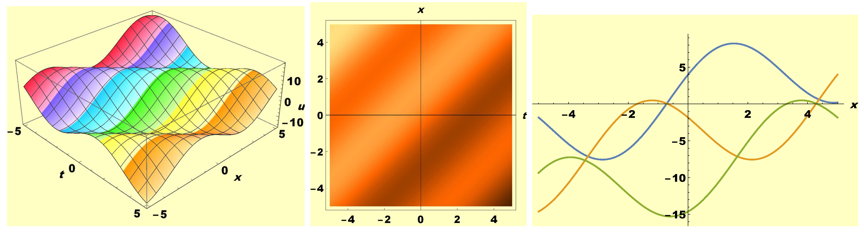
Figure 2.
Wave structure depiction of trigonometry solution (33) at .
Figure 2.
Wave structure depiction of trigonometry solution (33) at .
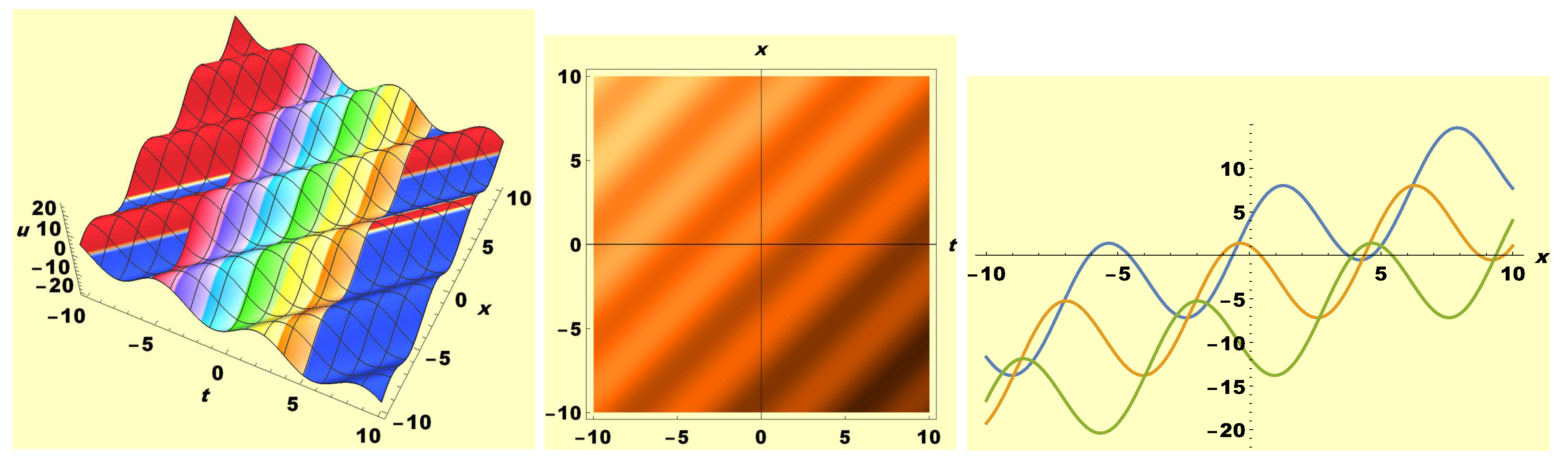
Figure 3.
Wave structure depiction of trigonometry solution (33) at .
Figure 3.
Wave structure depiction of trigonometry solution (33) at .
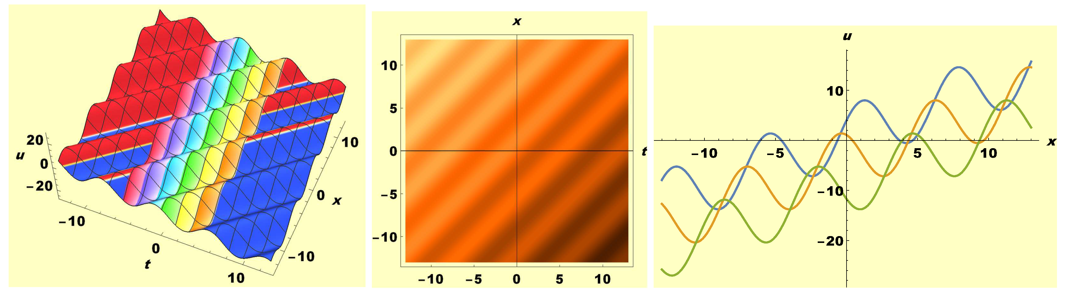
Figure 4.
Wave structure depiction of trigonometry solution (33) at .
Figure 4.
Wave structure depiction of trigonometry solution (33) at .
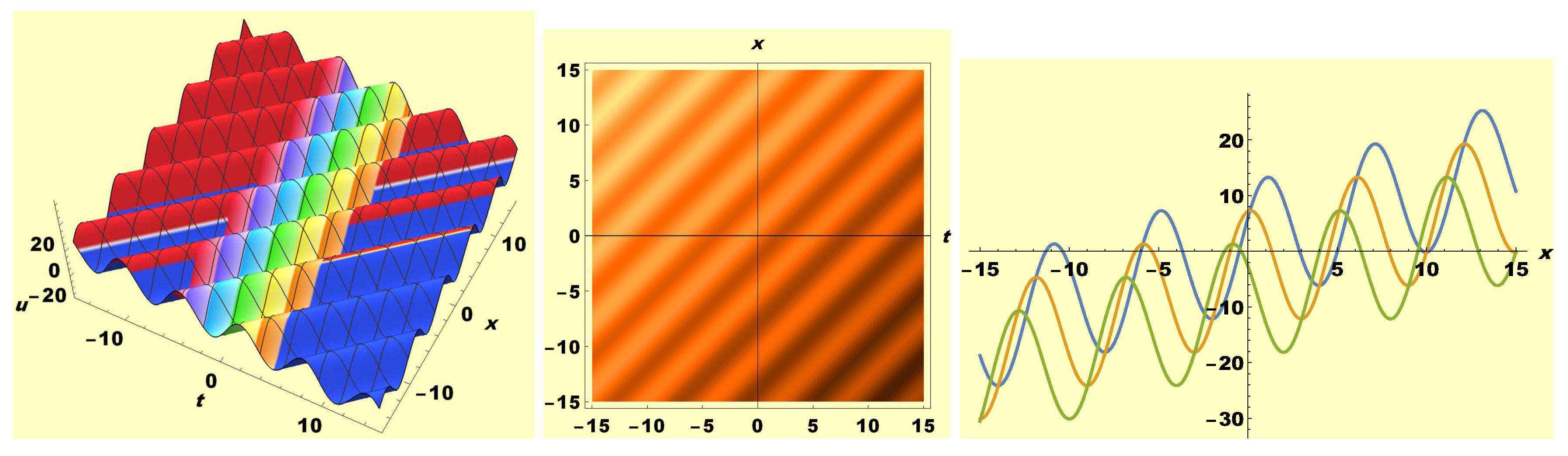
Figure 5.
Wave structure portrayal of log-trigonometric solution (45) at .
Figure 5.
Wave structure portrayal of log-trigonometric solution (45) at .
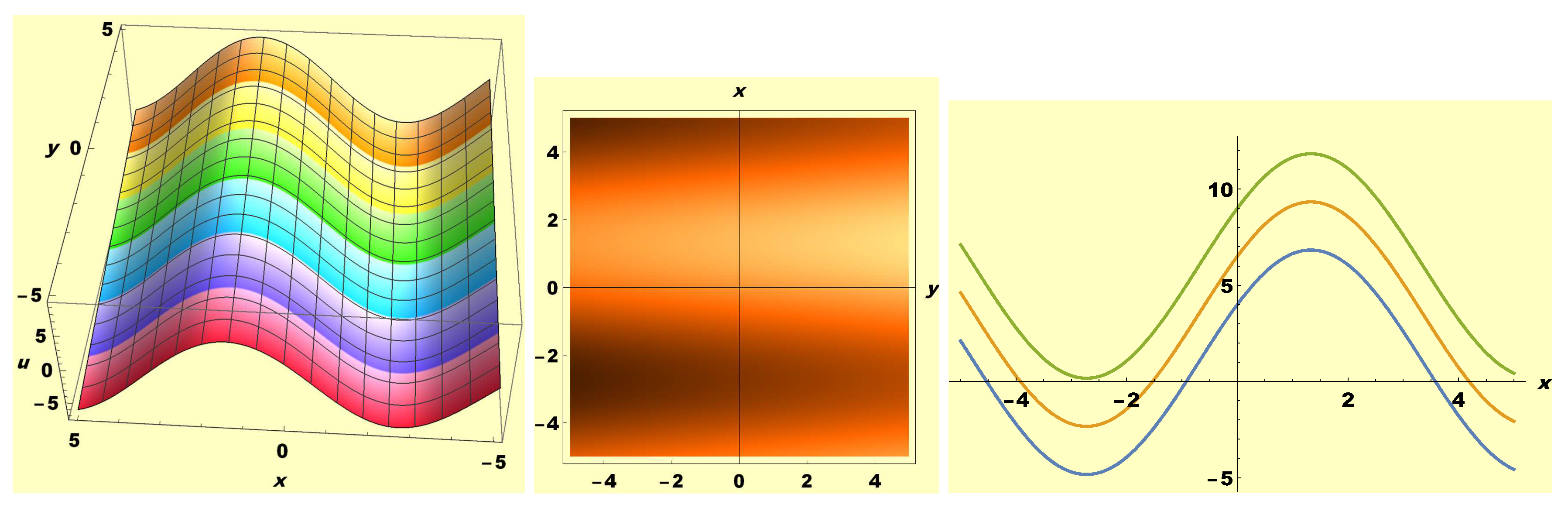
Figure 6.
Wave structure portrayal of log-trigonometric solution (45) at .
Figure 6.
Wave structure portrayal of log-trigonometric solution (45) at .
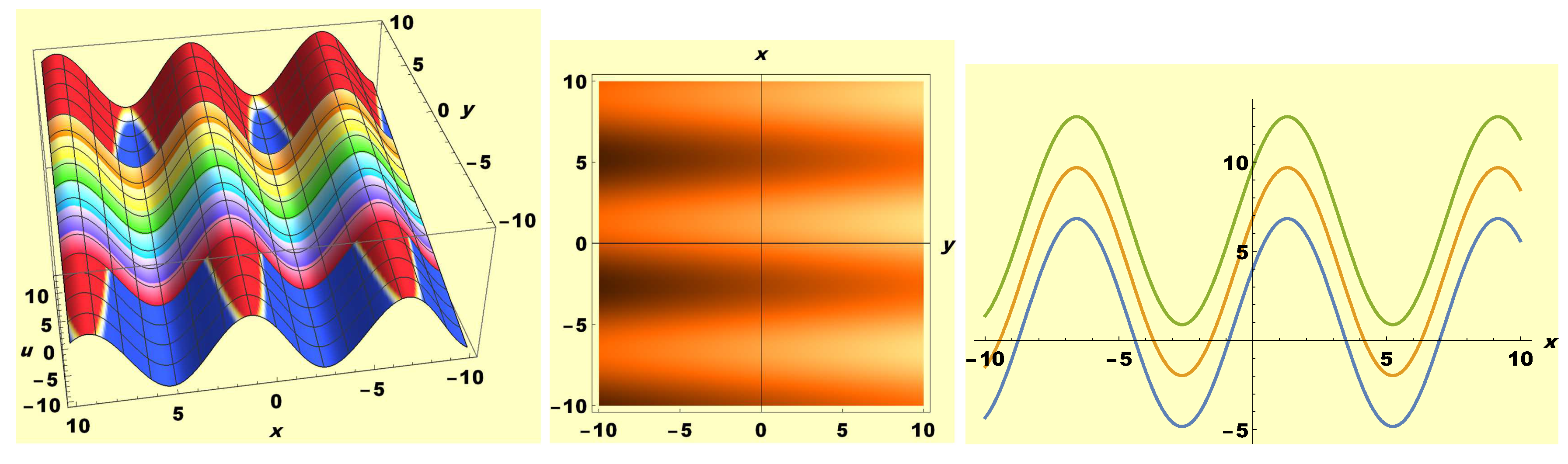
Figure 7.
Wave structure portrayal of log-trigonometric solution (45) at .
Figure 7.
Wave structure portrayal of log-trigonometric solution (45) at .
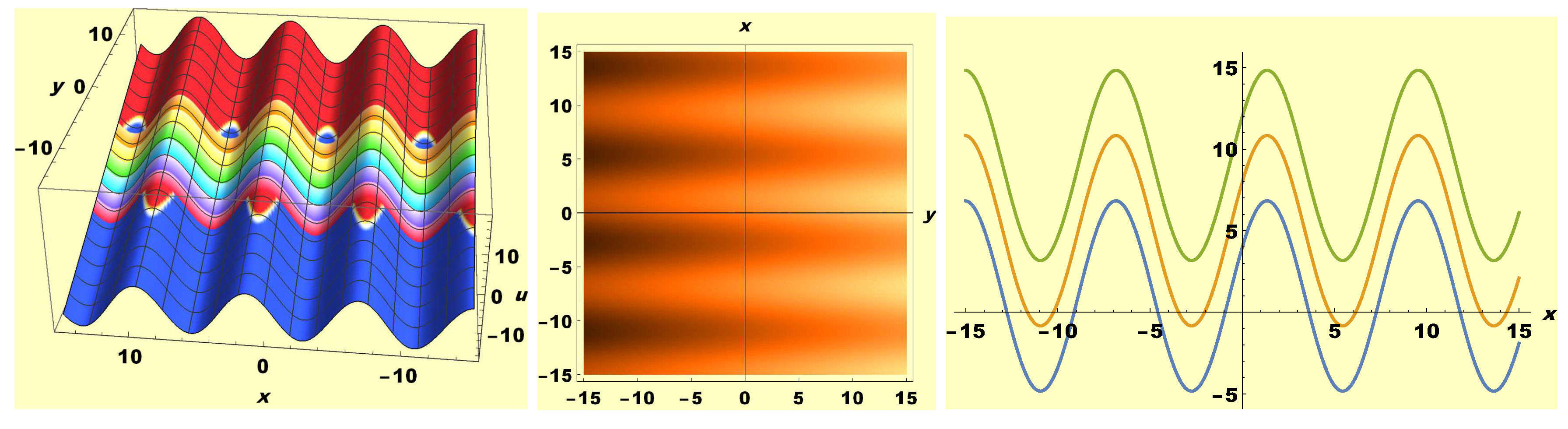
Figure 8.
Wave structure exhibition of hyperbolic solution (49) at .
Figure 8.
Wave structure exhibition of hyperbolic solution (49) at .
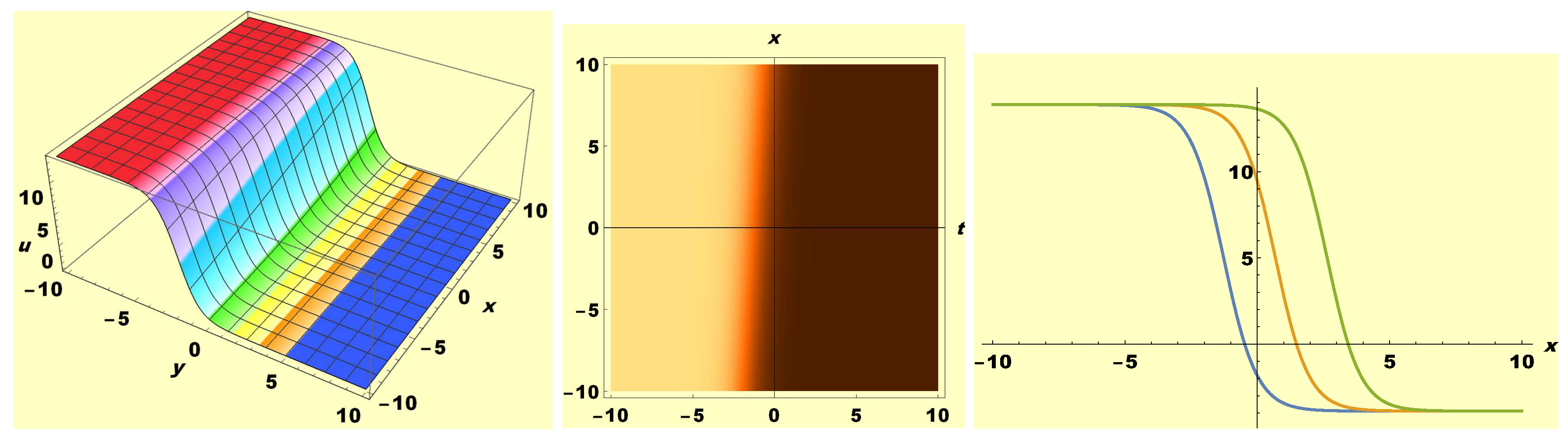
Figure 9.
Wave structure exhibition of hyperbolic solution (49) at .
Figure 9.
Wave structure exhibition of hyperbolic solution (49) at .
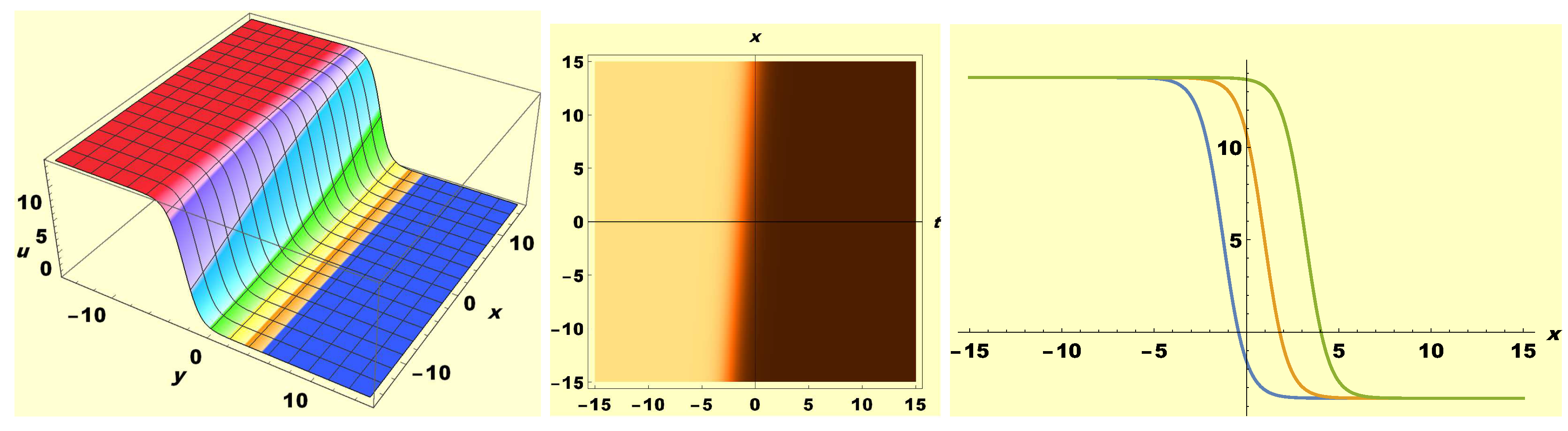
Figure 10.
Wave structure exhibition of hyperbolic solution (49) at .
Figure 10.
Wave structure exhibition of hyperbolic solution (49) at .
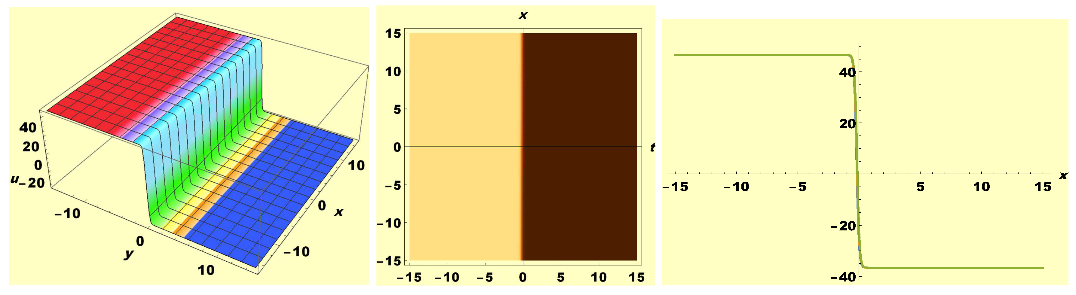
Figure 11.
Wave structure depicting the periodic soliton collisions at .
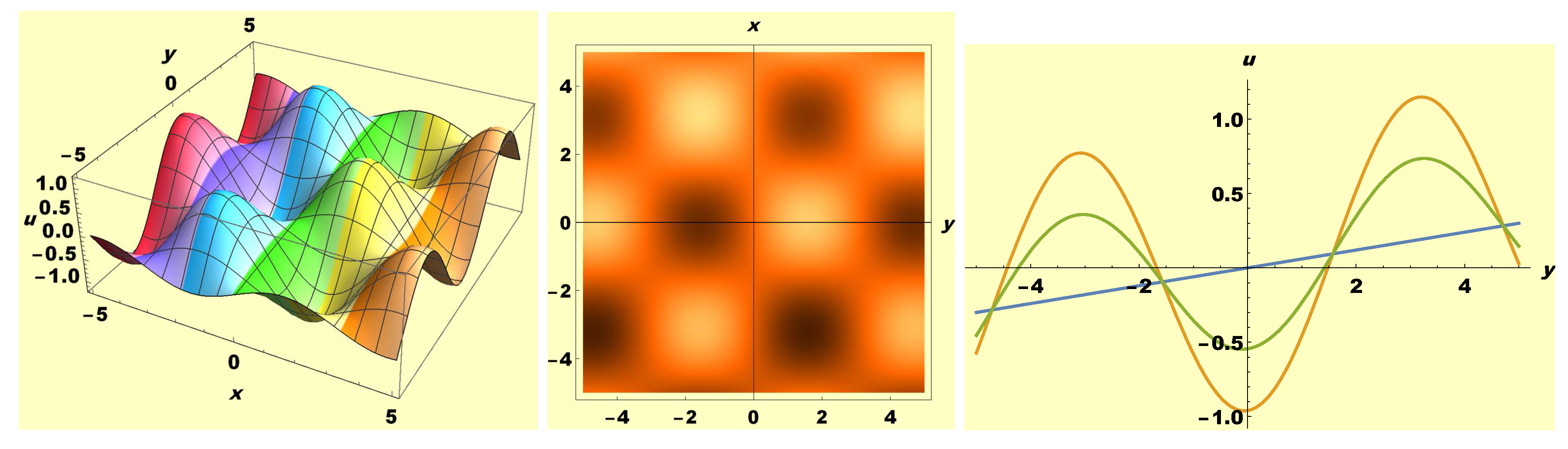
Figure 12.
Wave structure depicting the periodic soliton collisions at .
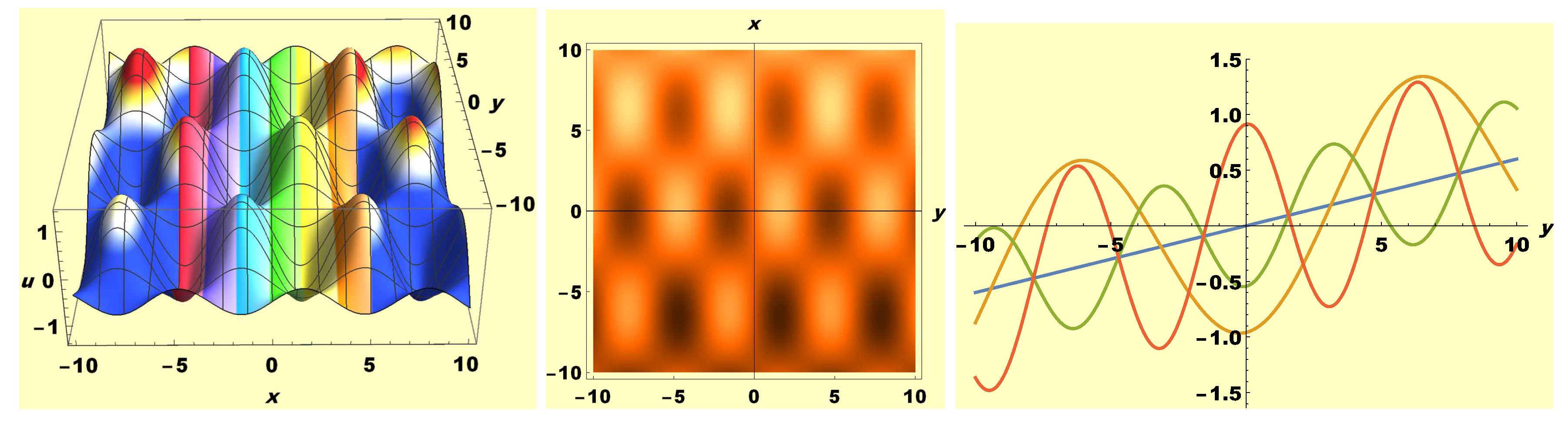
Figure 13.
Wave structure depicting the periodic soliton collisions at .
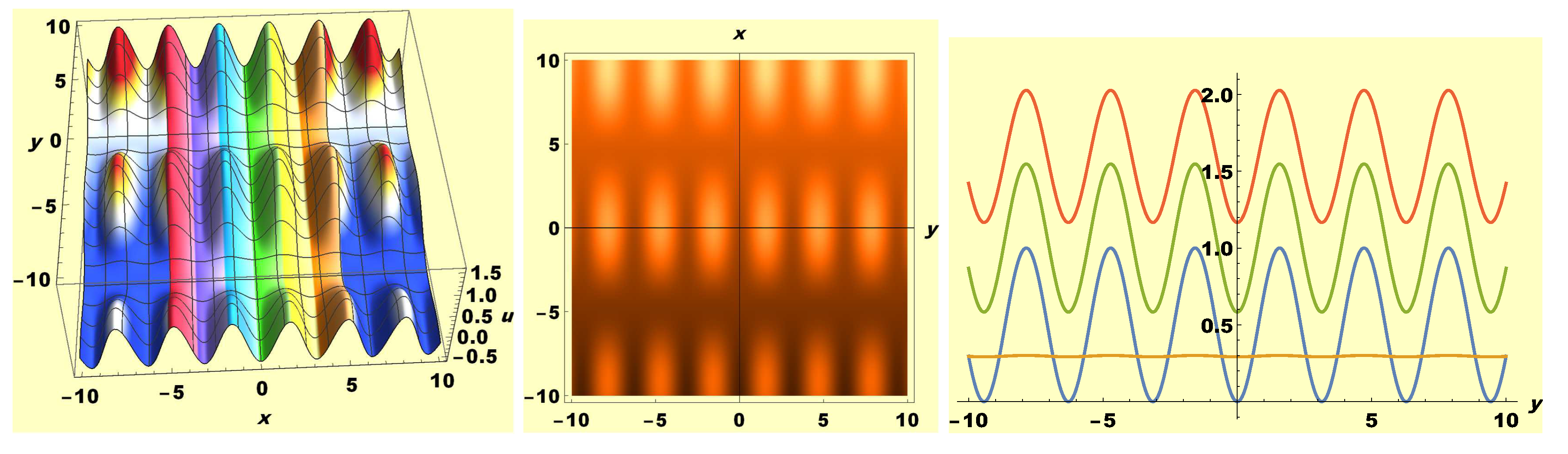
Figure 14.
Wave structure depicting the periodic soliton collisions at .
Disclaimer/Publisher’s Note: The statements, opinions and data contained in all publications are solely those of the individual author(s) and contributor(s) and not of MDPI and/or the editor(s). MDPI and/or the editor(s) disclaim responsibility for any injury to people or property resulting from any ideas, methods, instructions or products referred to in the content. |
© 2024 by the authors. Licensee MDPI, Basel, Switzerland. This article is an open access article distributed under the terms and conditions of the Creative Commons Attribution (CC BY) license (http://creativecommons.org/licenses/by/4.0/).
Copyright: This open access article is published under a Creative Commons CC BY 4.0 license, which permit the free download, distribution, and reuse, provided that the author and preprint are cited in any reuse.