1. Introduction
Angle’s classification is one of the most widely used in malocclusion classifications [
1]. Angle class I molar classification is determined by mesiobuccal cusp of the maxillary first molar occluding with the buccal groove of the mandibular first molar [
2]. Class I malocclusion was also categorized into five types by Dewey's modification. In Dewey type 1, anterior teeth are crowded, and in Dewey type 2, maxillary incisors are proclined. In type 3, there is an anterior crossbite, whereas in type 4, there is a posterior crossbite. Type 5 is characterized by permanent molars’ mesial drifts [
2,
3]. SCIIMO’s etiology is heterogeneous, because it can be caused by a mandibular retrusion, or maxillary protrusion, or both of them [
1]. Also, in SCIIMO, patients are categorized by the interarch relation. In a Class II molar relationship, the mesiobuccally cusp of the maxillary first permanent molar occludes mesial to the buccal groove of the mandibular first molar with correct inclination of the front teeth. Class II division 1 occurs when the maxillary incisors are protruded (upper incisors are proclined), often resulting in an excessive overjet and deep overbite. Class II division 2 occurs when the maxillary central incisors are palatally inclined and eventually overlapped by the maxillary lateral incisors. A deep overbite and a broad maxillary arch define a class II division 2 [
2].
Many approaches have been applied to diagnose craniofacial anatomy, commonly based on bidimensional imaging. In recent years, three-dimensional (3D) technologies have been developed, and more tools have been enabled in orthodontics [
3].
3D can define the occurrence of malocclusion: sagittal, transverse, and vertical [
4]. In the sagittal plane, the intermaxillary angle (SNA – SNB = ANB), which was recommended by Steiner 5 to determine an individual’s skeletal class, indicates SCIO if the ANB angle has values ranging between 0° and 4°, and SCIIMO if the ANB angle presents values >4° [
5,
6]. According to Jacobson [
7], the ANB angle does not consider the relative relationship of the denture bases to cranial reference planes. Due to this limitation, the “Wits” appraisal parameter was suggested, which overcomes this shortcoming and enables the measurement of the severity of the degree of anteroposterior jaw disharmony from lateral cephalograms [
7,
8]. In the following years, many studies presented equations that consider the individual properties of the ANB angle and Wits appraisal [
9,
10,
11,
12,
13] .
In summary, all traditional skeletal classifications depend on manually calculating linear and angular variables using the craniomaxillary and mandibular landmarks. However, due to variations in the mandible’s position that can be a result of occlusion and temporomandibular joint, skeletal classification can be difficult [
14]. To overcome these difficulties, classification algorithms like the support vector machine (SVM) can generate skeletal classifications based on the automatically extracted craniomaxillary variables [
14,
15]. Another study that examined automated skeletal classification found that convolutional neural networks (CNN), using the patient’s sex and a cephalogram, exhibited >90% sensitivity, specificity, and accuracy for vertical and sagittal skeletal diagnosis [
16]. Taraji et al. [
17], used cephalometric parameters, along with covariates such as gender, age, and race, to appraise machine-learning algorithms for adult Class III malocclusion treatment planning. Taraji et al. [
17] study demonstrated that artificial neural network algorithms predicted treatment approach with 91% accuracy. The model highlighted Wit's appraisal, anterior overjet, and Mx/Md ratio as key predictors.
In a scoping review that evaluated the use of artificial intelligence in orthodontics, and included 62 studies, demonstrated that the majority of the studies originated from the USA, South Korea, Japan and China. In addition, the review revealed that diagnosis and treatment planning field, was one of the most major domains that were investigated [
18].
Therefore, the main aim of this study was to derive a novel classification machine learning (ML) model to predict whether it’s SCIO or SCIIMO malocclusion among Palestinian Arab residents of Israel patients, using lateral cephalogram parameters, in addition to gender and age as covariates. This population can be considered a permanent population of this area, with family histories dating back for generations and high levels of consanguinity.
To our knowledge, this research will be the first to apply machine-learning models to this ethnic group. As a secondary outcome, a clustering analysis was intended to represent the data in clusters and to examine the differences between these clusters.
2. Material and Methods
2.1. Ethical Statement
This research was conducted according to current guidelines of the ethics and regulations of the Ethics Committee of the University of XXXXX (approval number 19-1596-101 (dated 13.11.2019)). This study consisted of 394 coded records of Palestinian Arab citizens of Israel who were diagnosed as SCIO or SCIIMO. All information collected as part of the standard of care by the orthodontists’ team at the XXXX.
The inclusion criteria were:
Calculated_ANB is defined as equal to ANB measured – ANB
ind. The ANB
ind was defined by Panagiotidis and Witt [
9]: ANB
ind = -35.16 + (0.4 x SNA) + (0.2 x ML-NSL).
In some cases, patients were included as SCIO or SCIIMO, even when the Calculated_ANB was not in the accepted range, according to clinical diagnosis and other important parameters, like the ANB angle and Wits appraisal. The fact that the Calculated_ANB is not suitable for all patients was described by Panagiotidis and Witt [
9].
- 2.
Available pre-treatment cephalometric data.
In this study, we performed a clustering analysis. In addition, we applied various ML algorithms, which differed in the number of input variables, enabling us to precisely classify the patients as skeletal class I or II via automatic machine learning techniques.
2.2. Cephalometric Variables
The following cephalometric parameters were the essential variables in this study analysis, and the complete information and location of all the parameters are presented in Supplementary
Table 1 and Supplementary
Figure 1.
2.3. Clustering Analysis
Data was analyzed using the R software platform, Clustering Analysis. Before starting the process of clustering, we conducted scaling process to reach a common scale.
The clustering algorithm was performed for 3 clusters, including SCIIMO or SCIO patients (separately). A scatter plot and dendrogram were produced using the R statistical program to implement the visualization of the cluster analysis results. We got the optimal cluster number by inspecting the dendrogram of different clusters.
To implement a hierarchical clustering algorithm, one has to choose a linkage function that defines the distance between any two sub-sets [
19]. In all our clustering calculations, we mainly used the Ward error sum of squares hierarchical clustering method that has been commonly used since its first description by Ward in 1963 [
20].
The performance of the machine learning models was evaluated by determining the accuracy and kappa scores.
2.4. Machine Learning Methods
Machine-learning analysis was applied using the R package Caret [
21]. Before starting this analysis, we preprocessed the data with centering and scaling functions to reach a standard scale and to improve the performance of the models.
2.5. Classification Models
Classification models - Linear Discriminant Analysis (LDA), Support Vector Machine (SVM), K Nearest Neighbor (KNN), Random Forest (RF), and Classification and Regression Tree (CART). They were all applied using the K-fold cross-validation (K=10).
2.6. Linear Discriminant Analysis (LDA)
LDA was proposed by R. Fischer in 1936. It consists of finding the projection hyperplane that minimizes the interclass variance and maximizes the distance between the projected means of the classes [
22].
2.7. Support Vector Machine (SVM)
The machine conceptually implements the idea that input vectors are non-linearly mapped to a high-dimension feature space. In this feature space, a linear decision surface is constructed [
23]. This model can be relatively simple and flexible for addressing various classification problems. SVMs afford balanced predictive performance distinctively, even in studies with limited sample sizes [
24].
2.8. K-Nearest Neighbors (KNN)
The nearest neighbor decision rule assigns an unclassified sample point to the classification of the nearest of a set of previously classified points. The k defines how many nearest neighbors need to be examined to classify the class of a sample point [
25,
26,
27]. This study used accuracy to select the optimal model using the largest k-value. The final value used for the general model (all parameters), model 1 (ANB angle), and model 2 (ANB angle and Wits appraisal), was 9 (k=9), while the model without the ANB parameters was k=5 (5 neighbors).
2.9. Random Forest (RF)
It is a classification method that uses many decision trees. This algorithm is a combination of tree predictors such that each tree depends on the values of a random vector sampled independently and with the same distribution for all trees in the forest [
27,
28].
2.10. Classification and Regression Tree (CART).
CART analysis is a form of binary recursive partitioning. In this method, each group of patients, represented by a “node” in a decision tree, can only be split into two groups. Each parent node can be split into two child nodes. The term “partitioning” refers to the fact that the dataset is split into sections or partitioned. It’s important to know that CART can handle numerical data that are highly skewed or multi-modal, as well as categorical
[29].
2.11. Model Validation
We divided our data into 70% for training and 30% of the data for validation (unseen data). We validated our models using the k-fold cross-validation approach. Cross-validation provides a simple and effective method for both model selection and performance evaluation; under k-fold cross-validation, the data are randomly partitioned to form k-disjoint subsets of approximately equal size [
30,
31]. K (10)-fold cross-validation was employed in this research. For conducting the ML models and calculating the Accuracy, Kappa, Receiver-operating characteristic curve (ROC), Sensitivity, and specificity scores, we used the R package Caret [
21].
3. Results
This study included 394 patients, with 157 (39.8%) presenting SCIO and 237 (60.2%) SCIIMO. The total study collective consisted of patients aged between 7 and 55 years, with a mean age of 19 ± 7.1 years in class I and 17 ± 6.5 years in class II cases. Concerning the gender distribution, among SCIO patients, 66% were female (n = 104), and in class II 67% were female (n = 158). The characteristics of the study collective, including demographic and cephalometric data, are presented in Supplementary Tables 2A-B for SCIO and SCIIMO patients, respectively.
3.1. Clustering
In this section, we performed hierarchical clustering analysis, and we inspected the number of clusters according to the dendrogram result. It was acceptable to present the current results with k=2,3 and 4 clusters. However, we decided to describe the k=3 clusters and show the distinct variations between the clusters. The same analysis was performed for skeletal class I and II separately.
3.2. Skeletal Class I Occlusion (SCIO) Clustering
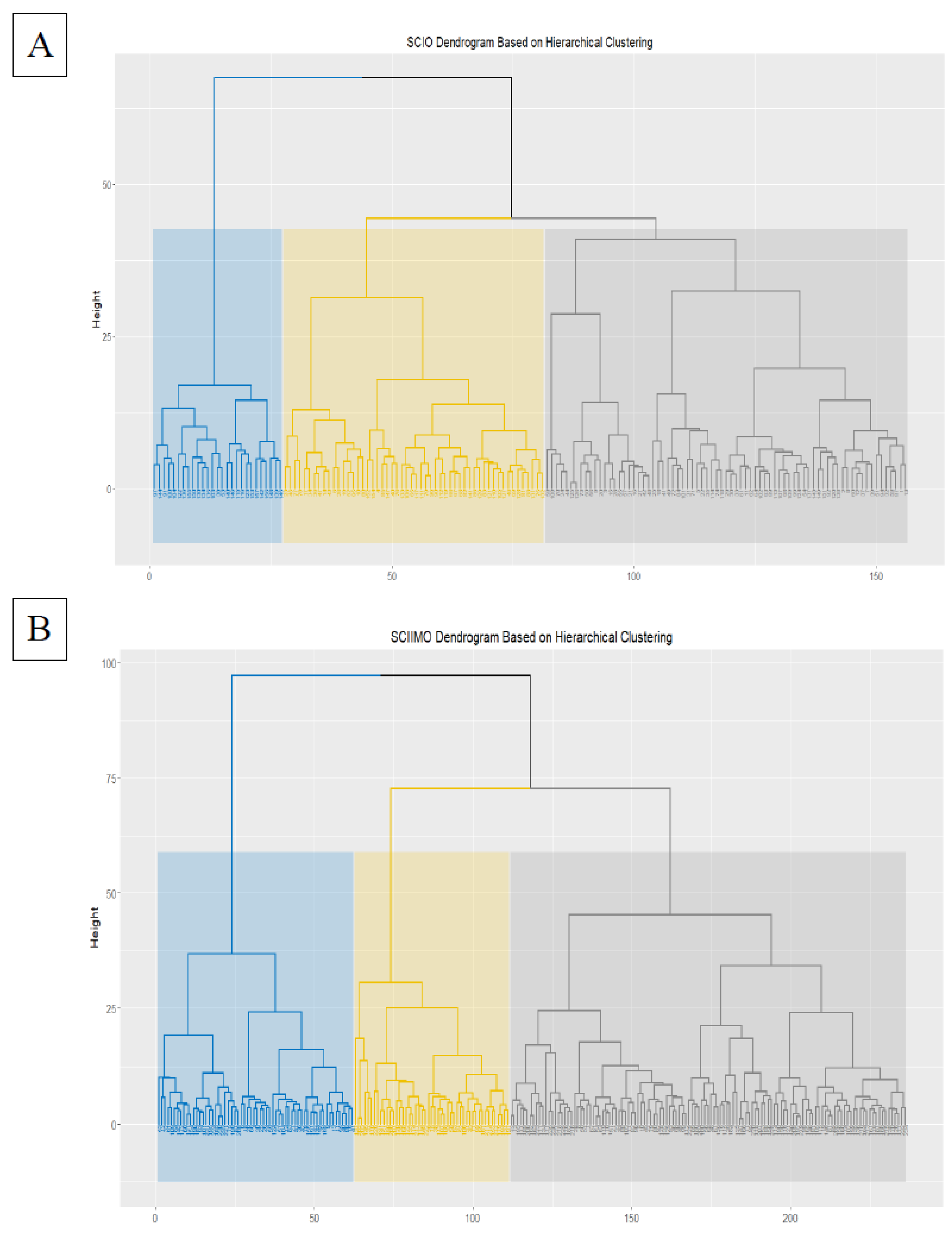
The hierarchical clustering results showed that the majority of patients were assigned to cluster 1 consisted of 75 (n=75) patients, and cluster 2 (n=54), while 27 patients (n=27) were assigned to the third cluster (
Figure 1A &
Table 1A).
In addition, the three clusters interestingly variated significantly (P<0.05) in all cephalometric parameters except in the parameters (Calculated_ANB and Wits appraisal, P>0.05). Besides, from the results, age differences were not significant between the three clusters. The results showed that in the second cluster, retrognathism of the mandible was less severe, as represented by a a lower ANB angle. In addition, the third cluster had a lower NL-ML angle, gonial angle, SN-Ba angle, and lower ML-NSL angle compared to clusters 1 and 2, which demonstrate the distinct features from the other two clusters. Detailed information can be found on
Table 1B.
We repeated the same clustering analysis with males and females separately and found that there are some similar patterns, like the fact that in both males and females, the second cluster was characterized by less severe retrognathism of the mandible, as represented by a lower ANB angle. However, the results also showed variations between males and females. For instance, most dental parameter variations were not significant between the three clusters among males, and significant among females clustering. The results showed that age was insignificant between clusters for both males and females. Overall, females showed more significant differences among clusters among the cephalometric parameters (
Table 1C).
3.3. Skeletal Class II Malocclusion (SCIIMO) Clustering
In skeletal class II hierarchical clustering, the results showed that the majority of patients were assigned to cluster 1, consisting of 125 (n=125) patients. In contrast, 111 patients (cluster 2, n=62, cluster 3, n=49) were assigned the second and third clusters (
Figure 1B &
Table 1A).
In addition, the three clusters interestingly variated significantly (P<0.05). Also, here, among skeletal class II patients, age differences in the different clusters were not significant. Interestingly, the results showed a significant among most of the sagittal parameters, especially the ANB angle and the Calculated_ANB. The results showed that the second cluster has less severe retrognathism of the mandible, which is represented by a lower ANB angle and Calculated_ANB and a higher SNB angle (P<0.05). Detailed information can be found in
Table 1D.
Finally, we repeated the same clustering analysis with males and females separately and found that age differences were significant between clusters for males and females (P<0.05). Cluster 1 here was characterized by a younger age average M=12.90 (M=12.90, SD=2.20) among males, and M=15.88 (M=15.88, SD=5.11). For both males and females, the results showed that the first cluster has less severe retrognathism of the mandible, which is represented by a lower ANB angle and Calculated_ANB (significant among males only, P<0.05), compared to the other two clusters. In addition, and on the contrary to skeletal class I, here Wits appraisal variations were significant between the clusters for both males and females (P<0.05), and was lower in the first cluster, compared to the other two clusters. Overall, also among skeletal class II patients, females showed more significant differences among clusters among the cephalometric parameters (
Table 1E).
3.4. Machine Learning Models
Considering the knowledge about cephalometric measurements in SCIO and SCIIMO obtained from cluster analysis and comparisons of cephalometric parameters between subgroups, various machine learning models were tested to predict the classification of an individual based on machine learning (ML) models that will not be based on the Calculated_ANB (model 3).
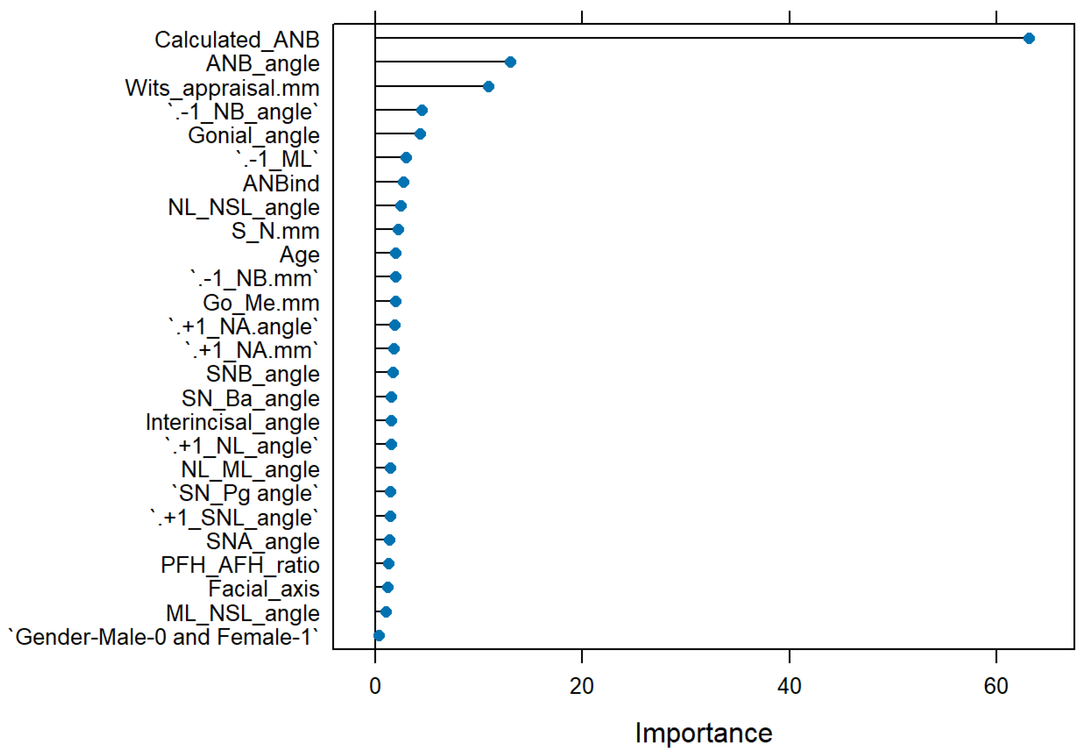
The general ML model, which included all cephalometric and demographic parameters, could predict a SCIO or SCIIMO with an accuracy of 0.87 (0.87%) (RF, Accuracy = 0.87, Kappa = 0.74, ROC = 0.92, Sensitivity = 0.92, and Specificity = 0.83). As expected, calculated_ANB was the most critical parameter in the model, followed by Wits appraisal, ANB, -1/NB, and gonial angle, as shown in
Figure 2.
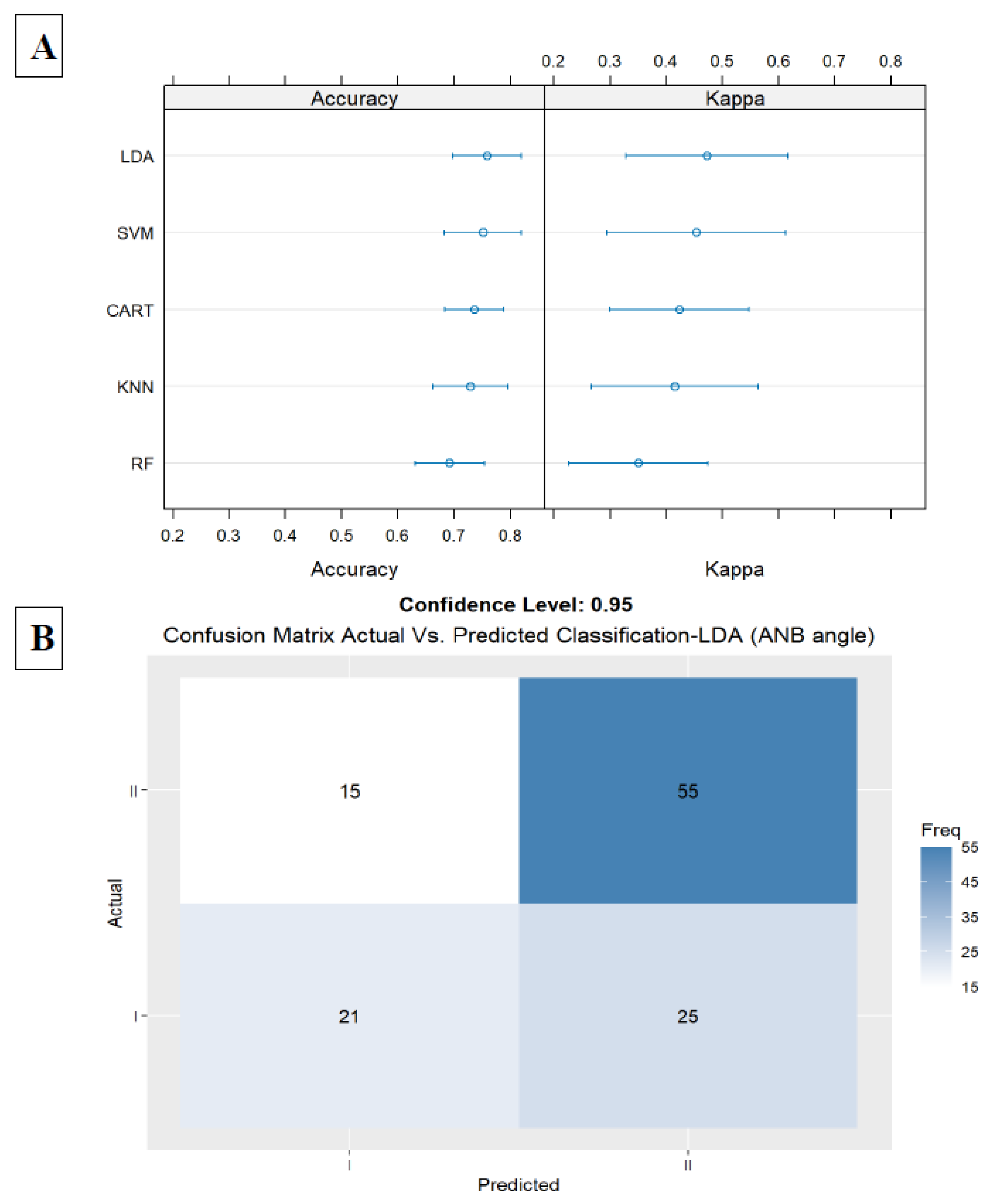
The first model included only the ANB angle, the second important parameter in the general model. In this model, we received an accuracy of 0.75 (LDA, Accuracy = 0.75, Kappa = 0.47, ROC = 0.79, Sensitivity = 0.59, and Specificity = 0.86). Results are presented in
Figure 3A,B
.
The second model included the ANB angle, and the Wits appraisal, which improved the accuracy to 0.78 in the KNN model (KNN, Accuracy = 0.78, Kappa = 0.56, ROC = 0.82, Sensitivity = 0.80, and Specificity = 0.76) (
Figure 4A,B). A decision tree visualization for these two parameters is presented in
Figure 4C. Finally, adding the third model (model 3) included all parameters except for ANB, ANB
ind, and Calculated_ANB and achieved 0.82 accuracy in the LDA model (LDA, Accuracy = 0.82, Kappa = 0.63, ROC = 0.88, Sensitivity = 0.75, and Specificity = 0.87). In addition, we examined the classification ability without ANB, ANB
ind, and Calculated_ANB parameters via decision tree, which showed that the tree starts with Wits appraisal, followed by SNB, NL-NSL, +1/NA (mm), and age in the first three branches (
Figure 5A–D). A summary of all the ML models is available in
Table 2.
4. Discussion
Our study aimed to reveal novel information about the Palestinian Arab ethnic minority who are citizens of Israel. Hierarchical clustering analysis was performed separately for both skeletal class I and II patients, and based on the dendrogram we decided to apply 3 clusters for every analysis. Among skeletal class I patients, three distinct patterns were revealed. The second cluster was characterized with less severe retrognathism. For skeletal class II patients, we also applied hierarchical clustering for three clusters, and here also the results showed a significant among most of the sagittal parameters, especially, the ANB angle, and the Calculated_ANB. The results showed that the second cluster has less severe retrognathism of the mandible which is represented by a lower ANB angle and Calculated_ANB, and higher SNB angle. Interestingly, age differences were significant between clusters, among males and females.
In a study that was done by Moreno Uribe et al.[
32] about phenotypic diversity in white adults with Class II malocclusion, it was found that models with 2, 3, or 4 clusters were statistically acceptable. Still, in the end, they identified five distinct Class II phenotypes [
32].
A Cluster analysis study in Class I occlusion revealed that the grouping pattern in Class I occlusion is present at younger age levels and disappears with age. Also, they found that the clustering pattern is very similar in males and females with Class I occlusion [
33].
Finally, the general ML model that included all parameters could predict an individual as SCIO or SCIIMO with 0.87 accuracy (RF, Accuracy = 0.87, Kappa = 0.74, ROC = 0.92, Sensitivity = 0.92, and Specificity = 0.83). As expected, Calculated_ANB was the most critical parameter in the model, followed by ANB angle, Wits appraisal, and ANBind. Our Machine Learning results demonstrated that with the ANB angle and the Wits appraisal, two cephalometric parameters can predict skeletal class I/ II with 0.78 accuracy (KNN, Accuracy = 0.78, Kappa = 0.56, ROC = 0.82, Sensitivity = 0.80, and Specificity = 0.76). In addition, our third model (model 3) included all parameters except for ANB, ANBind, and Calculated_ANB and achieved 0.82 accuracy in the LDA model (LDA, Accuracy = 0.82, Kappa = 0.63, ROC = 0.88, Sensitivity = 0.75, and Specificity = 0.87).
In recent research that was conducted by Midlej et al. [
34] and aimed to accurately classify individual Arab patients, being citizens of Israel, as skeletal class II or III, found that Wits appraisal and SNB angle were able to predict the classification of patients to either skeletal class II or III with an accuracy of 0.95.
Jayathilake et al. [
35] examined the prediction of malocclusion patterns using a classification model. Their study considered SNA, SNB, and ANB as cephalometric variables. The patients were classified into malocclusion patterns according to the ANB angle (pattern I, II, and III). The authors found that the accuracy of the multinomial logistic regression model, K-NN algorithm, random forest, and Naïve Bayes classification of malocclusion patterns were 88.89%, 83.33%, 88.89%, and 55.56%, respectively.
In another study that aimed to accurately diagnose skeletal class-III malocclusion applied through mobile images, and used three models: a deep learning algorithm, a machine learning algorithm, and a rule-based algorithm, found that the best model was able to correctly classify skeletal class-III malocclusion, with an accuracy of 76% [36].
4.1. Traditional vs. New Machine Learning Methods
When comparing the performance of ML models compared to traditional diagnostic approaches, like the Calculated_ANB formula that we used in this article to classify the patients. We need to consider that this regression formula (Calculated_ANB) and others, don’t fit all cases. In many cases, patients are diagnosed clinically, and according to other cephalometric parameters, like ANB angle and Wits appraisal. Panagiotidis and Witt [
9] investigated this limitation by the correlation coefficient of the ANB
ind equation, as r = 0.808. In addition, the available individualized were established based on specific populations, that consider the individual properties of the ANB angle and Wits appraisal [
9,
10,
11,
12,
13]. On the other hand, this research and other studies suggest to apply uniform machine learning algorithms, that can be trained on one ethnic group, like this study, or future studies that will aim to combine different ethnicities models.
4.2. Limitations
This study applied clustering analysis only on three clusters. Although the results showed significant patterns within each skeletal class, further investigations for different cluster numbers could be done. This study used a machine learning model based on a moderate sample size, and future studies should consider increasing it. Furthermore, our results were drawn from specific populations, and the results might vary among other populations. Finally, future research should aim to include all skeletal malocclusion classifications, and not only skeletal class I and II.
4.3. Conclusion and Future Research
This research revealed new information regarding the distinct characteristics of each cluster within each patient group (SCIO/SCIIMO) based on various cephalometric parameters.
Among skeletal class I patients, three distinct patterns were revealed. The second cluster was characterized by less severe retrognathism. Regarding skeletal class II patients, the three clusters showed significant differences among most of the sagittal parameters. The results showed that the second cluster has less severe retrognathism of the mandible which is represented by a lower ANB angle and Calculated_ANB, and higher SNB angle. Interestingly, age differences were significant between clusters, among males and females on in SCIIMO patients. These results can have implications both on the diagnosis and treatment plan
The ML models showed a high ability to predict a SCIO or SCIIMO with an accuracy of 0.87 (RF, Accuracy = 0.87, Kappa = 0.74, ROC = 0.92, Sensitivity = 0.92, and Specificity = 0.83) in the general model and a 0.78 accuracy (KNN, Accuracy = 0.78, Kappa = 0.56, ROC = 0.82, Sensitivity = 0.80, and Specificity = 0.76) using Wits appraisal and ANB angle. The study presents a machine learning model as a promising universal approach for precise and fast skeletal class I/ II diagnosis, advancing personalized orthodontic diagnostics and treatment. Finally, further research is recommended to be done, on applying artificial intelligence and machine-learning methods on the treatment choices and outcomes.
Author Contributions
Conceptualization. F.A.I., P.P., and N.W.; methodology. K.M., I.M.L., O.Z., O.A., S.M., S.K., E.P.S, A.N., and C.K.; validation. F.A.I.; investigation. K.M., I.M.L., O.Z., N.W., O.A., S.M., S.K.. and C.K.; resources. F.A.I., P.P., N.W., S.K. K.M., and C.K.; data curation. K.M., I.M.L., and O.Z.; writing—original draft preparation. K.M., I.M.L., O.Z., F.A.I.; writing—review and editing. K.M., I.M.L., O.Z., O.A., S.M., S.K., A.N., E.P.S., C.K., P.P., N.W., and F.A.I.; supervision. F.A.I. P.P. and N.W.; project administration. F.A.I.; funding acquisition. F.A.I. P.P. and N.W. All authors have read and agreed to the published version of the manuscript.
Funding
This study was supported by a core fund from Tel Aviv University, the Orthodontic Research Center, and the University Hospital of Regensburg.
Institutional Review Board Statement
According to current guidelines and following the Ethics Committee of the University of Regensburg ethics and regulations. The committee reviewed and approved this research project and study design with approval number 19-1596-101 (dated 13.11.2019).
Informed Consent Statement
Informed consent was obtained from all subjects involved in the study.
Data Availability Statement
The data that support the findings of this study are available on request from the corresponding author.
Conflicts of Interest
The authors declare no conflict of interest.
References
- Lone, I.M.; Zohud, O.; Midlej, K.; Proff, P.; Watted, N.; Iraqi, F.A. Skeletal Class II Malocclusion: From Clinical Treatment Strategies to the Roadmap in Identifying the Genetic Bases of Development in Humans with the Support of the Collaborative Cross Mouse Population. Journal of Clinical Medicine 2023, 12, 5148. [Google Scholar] [CrossRef] [PubMed]
- Ghodasra, R.; Brizuela, M. Orthodontics, Malocclusion. StatPearls 2023.
- Francisco, I.; Ribeiro, M.P.; Marques, F.; Travassos, R.; Nunes, C.; Pereira, F.; Caramelo, F.; Paula, A.B.; Vale, F. Application of Three-Dimensional Digital Technology in Orthodontics: The State of the Art. Biomimetics 2022, 7, 23. [Google Scholar] [CrossRef] [PubMed]
- Cenzato, N.; Nobili, A.; Maspero, C. Prevalence of Dental Malocclusions in Different Geographical Areas: Scoping Review. Dent J (Basel) 2021, 9. [Google Scholar] [CrossRef]
- Steiner, C.C. Cephalometrics for You and Me. Am J Orthod 1953, 39. [Google Scholar] [CrossRef]
- Avelar Fernandez, C.C.; Cruz Alves Pereira, C.V.; Luiz, R.R.; Vieira, A.R.; De Castro Costa, M. Dental Anomalies in Different Growth and Skeletal Malocclusion Patterns. Angle Orthodontist 2018, 88. [Google Scholar] [CrossRef]
- Jacobson, A. Application of the “Wits” Appraisal. Am J Orthod 1976, 70. [Google Scholar] [CrossRef]
- Armed, P.; Jan, A.; Bangash, A.; Shinwari, S.; Pakistan, R. THE CORRELATION BETWEEN WITS AND ANB CEPHALOMETRIC LANDMARKS IN ORTHODONTIC PATEINTS. Pakistan Armed Forces Medical Journal 2017, 67, S267–71. [Google Scholar]
- Panagiotidis, G.; Witt, E. Der Individualisierte ANB-Winkel. Fortschr Kieferorthop 1977, 38. [Google Scholar] [CrossRef]
- Järvinen, S. Floating Norms for the ANB Angle as Guidance for Clinical Considerations. American Journal of Orthodontics and Dentofacial Orthopedics 1986, 90. [Google Scholar] [CrossRef]
- Järvinen, S. Relation of the Wits Appraisal to the ANB Angle: A Statistical Appraisal. American Journal of Orthodontics and Dentofacial Orthopedics 1988, 94. [Google Scholar] [CrossRef]
- Yen, C.H. The Individualized ANB Angle of Chinese Adults. Kaohsiung Journal of Medical Sciences 1990, 6. [Google Scholar]
- Paddenberg, E.; Proff, P.; Kirschneck, C. Floating Norms for Individualising the ANB Angle and the WITS Appraisal in Orthodontic Cephalometric Analysis Based on Guiding Variables. Journal of Orofacial Orthopedics 2023, 84. [Google Scholar] [CrossRef] [PubMed]
- Liu, J.; Chen, Y.; Li, S.; Zhao, Z.; Wu, Z. Machine Learning in Orthodontics: Challenges and Perspectives. Advances in Clinical and Experimental Medicine 2021, 30. [Google Scholar] [CrossRef] [PubMed]
- Niño-Sandoval, T.C.; Guevara Perez, S. V.; González, F.A.; Jaque, R.A.; Infante-Contreras, C. An Automatic Method for Skeletal Patterns Classification Using Craniomaxillary Variables on a Colombian Population. Forensic Sci Int 2016, 261, 159.e1–159.e6. [Google Scholar] [CrossRef]
- Yu, H.J.; Cho, S.R.; Kim, M.J.; Kim, W.H.; Kim, J.W.; Choi, J. Automated Skeletal Classification with Lateral Cephalometry Based on Artificial Intelligence. J Dent Res 2020, 99, 249–256. [Google Scholar] [CrossRef]
- Taraji, S.; Atici, S.F.; Viana, G.; Kusnoto, B.; Allareddy, V. (Sath); Miloro, M.; Elnagar, M.H. Novel Machine Learning Algorithms for Prediction of Treatment Decisions in Adult Patients With Class III Malocclusion. Journal of Oral and Maxillofacial Surgery 2023, 81. [Google Scholar] [CrossRef]
- Bichu, Y.M.; Hansa, I.; Bichu, A.Y.; Premjani, P.; Flores-Mir, C.; Vaid, N.R. Applications of Artificial Intelligence and Machine Learning in Orthodontics: A Scoping Review. Prog Orthod 2021, 22. [Google Scholar] [CrossRef]
- Nielsen, F. Introduction to HPC with MPI for Data Science. Springer 2016.
- Murtagh, F.; Legendre, P. Ward’s Hierarchical Agglomerative Clustering Method: Which Algorithms Implement Ward’s Criterion? J Classif 2014, 31, 274–295. [Google Scholar] [CrossRef]
- Kuhn, M.; Wing, J.; Weston, S.; Williams, A.; Keefer, C.; Engelhardt, A.; Cooper, T.; Mayer, Z.; Kenkel, B.; Team, R.C.; et al. Package “Caret.” R J 2020.
- Xanthopoulos, P.; Pardalos, P.M.; Trafalis, T.B. Robust Data Mining. 2013. [CrossRef]
- Cortes, C.; Vapnik, V.; Saitta, L. Support-Vector Networks. Machine Learning 1995, 20, 273–297. [Google Scholar] [CrossRef]
- Pisner, D.A.; Schnyer, D.M. Support Vector Machine. Machine Learning: Methods and Applications to Brain Disorders 2020, 101–121. [CrossRef]
- Cover, T.M.; Hart, P.E. Nearest Neighbor Pattern Classification. IEEE Trans Inf Theory 1967, 13, 21–27. [Google Scholar] [CrossRef]
- Qahaz, N.; Lone, I.M.; Khadija, A.; Ghnaim, A.; Zohud, O.; Nun, N. Ben; Nashef, A.; Abu El-Naaj, I.; Iraqi, F.A. Host Genetic Background Effect on Body Weight Changes Influenced by Heterozygous Smad4 Knockout Using Collaborative Cross Mouse Population. Int J Mol Sci 2023, 24. [Google Scholar] [CrossRef] [PubMed]
- Lone, I.M.; Nun, N. Ben; Ghnaim, A.; Schaefer, A.S.; Houri-Haddad, Y.; Iraqi, F.A. High-Fat Diet and Oral Infection Induced Type 2 Diabetes and Obesity Development under Different Genetic Backgrounds. Animal Model Exp Med 2023, 6, 131–145. [Google Scholar] [CrossRef] [PubMed]
- Breiman, L. (Impo)Random Forests(Book). Mach Learn 2001.
- Lewis, R.J.; Ph, D.; Street, W.C. An Introduction to Classification and Regression Tree ( CART ) Analysis. 2000 Annual Meeting of the Society for Academic Emergency Medicine 2000.
- Cawley, G.C.; Talbot, N.L.C. On Over-Fitting in Model Selection and Subsequent Selection Bias in Performance Evaluation. Journal of Machine Learning Research 2010, 11. [Google Scholar]
- Lone, I.M.; Midlej, K.; Nun, N. Ben; Iraqi, F.A. Intestinal Cancer Development in Response to Oral Infection with High-Fat Diet-Induced Type 2 Diabetes (T2D) in Collaborative Cross Mice under Different Host Genetic Background Effects. Mamm Genome 2023, 34, 56–75. [Google Scholar] [CrossRef]
- Uribe, L.M.M.; Vela, K.C.; Kummet, C.; Dawson, D. V.; Southard, T.E. Phenotypic Diversity in White Adults with Moderate to Severe Class III Malocclusion. American Journal of Orthodontics and Dentofacial Orthopedics 2013, 144. [Google Scholar] [CrossRef]
- Espona, I.G.; Gomez, J.T.; Carmona, J.B. Cluster Analysis Application to Class I Malocclusion. Eur J Orthod 1995, 17, 231–240. [Google Scholar] [CrossRef]
- Midlej, K.; Watted, N.; Awadi, O.; Masarwa, S.; Lone, I.M.; Zohud, O.; Paddenberg, E.; Krohn, S.; Kuchler, E.; Proff, P.; et al. Lateral Cephalometric Parameters among Arab Skeletal Classes II and III Patients and Applying Machine Learning Models. Clin Oral Investig 2024, 28, 1–16. [Google Scholar] [CrossRef]
- AKSOY, S.; KILIÇ, B.; SÜZEK, T. COMPARATIVE ANALYSIS OF THREE MACHINE LEARNING MODELS FOR EARLY PREDICTION OF SKELETAL CLASS-III MALOCCLUSION FROM PROFILE PHOTOS. Mugla Journal of Science and Technology 2022, 8. [Google Scholar] [CrossRef]
Figure 1.
1A. Hierarchical clustering dendrogram for skeletal class I occlusion (SCIO) – the X axis (rows) represents patients clustering, which is divided into three main clusters with different colors, and the Y axis represents the distance between clusters. 1B. Hierarchical clustering dendrogram for skeletal class II malocclusion (SCIIMO) – the X axis (rows) represents patients clustering, which is divided into three main clusters with different colors, and the Y axis represents the distance between clusters.
Figure 2.
General Machine Learning model summary of the importance of each parameter to the model in predicting the classification of skeletal class I or II. The X-axis shows the importance of the prediction of the different assessed variables. The Y-axis shows the list of the assessed variables.
Figure 2.
General Machine Learning model summary of the importance of each parameter to the model in predicting the classification of skeletal class I or II. The X-axis shows the importance of the prediction of the different assessed variables. The Y-axis shows the list of the assessed variables.
Figure 3.
A. Summarize model 1 (one predictor) of the different Machine Learning models. This Figure presents a summary of the five Machine-Learning classification models, including Linear Discriminant Analysis (LDA), Support Vector Machine (SVM), K-Nearest Neighbors, Random Forest (RF), Classification, and Regression Tree (CART), and are presented in the Y-axis. The X-axis shows the Accuracy and Kappa scores for each model. The first model included the ANB angle only; in the LDA, we received an Accuracy of 0.75 and Kappa of 0.47. 3B. Summarize model 1 (one predictor) of the different Machine Learning models. It presents the LDA Machine Learning Model Confusion Matrix of the validation data (30% of the sample) for the ANB angle to predict the classification (Predicted) compared to the Actual classification, based on using this variable only. The X-axis shows the skeletal class I and II predictions, and the Y-axis shows the number of identified patients in each classification. .
Figure 4.
A. Summarize model 2 (two predictors) of the different Machine Learning models. This Figure presents a summary of the five Machine-Learning classification models tested, including Linear Discriminant Analysis (LDA), Support Vector Machine (SVM), K-Nearest Neighbors, Random Forest (RF), Classification and Regression Tree (CART) as presented on the Y-axis. The X-axis shows the Accuracy and Kappa scores for each model. B. The Machine Learning Model Confusion Matrix of the validation data shows the ability of the KNN model to predict the classification (Predicted) compared to the Actual classification based on the ANB angle and Wits appraisal. The X-axis shows the skeletal class I and II predictions, and the Y-axis indicates the number of identified patients in each classification. C. The second model tree diagram shows the decision rules of the model. The root node is at the top, and the leaf nodes are at the bottom. Each node is labeled with the cephalometric parameter used to split the data at that node, as well as the split value. The leaf nodes are labeled with the predicted class for the data that reaches that node.
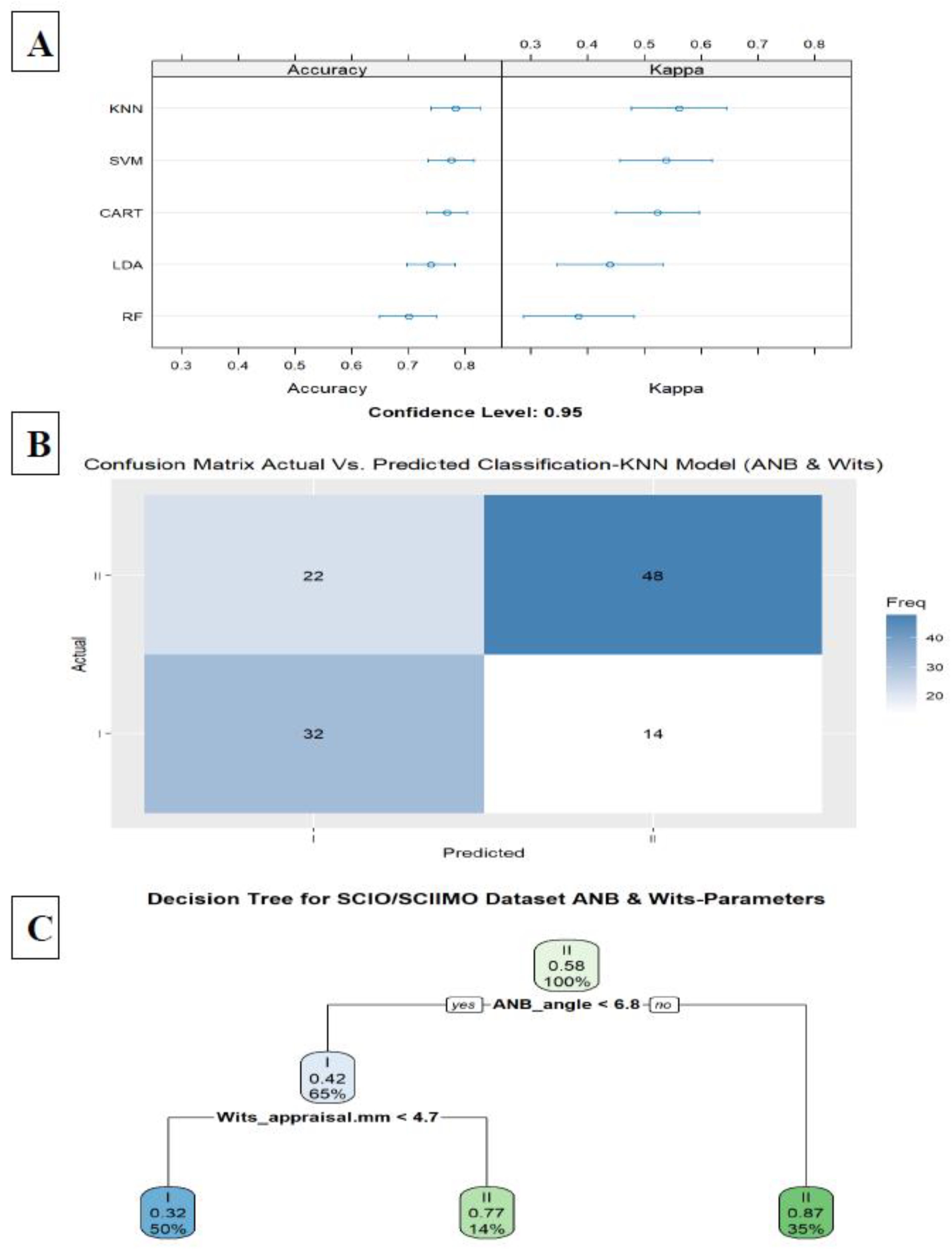
Figure 5.
A. Summarize model 3 (all parameters except ANB angle, ANBind, and Calculated_ANB) of the different Machine Learning models. This Figure presents a summary of the five Machine-Learning classification models tested, including Linear Discriminant Analysis (LDA), Support Vector Machine (SVM), K-Nearest Neighbors, Random Forest (RF), Classification and Regression Tree (CART) as presented on the Y-axis. The X-axis shows the Accuracy and Kappa scores for each model. B. Model 3 summarizes the importance of each parameter to the model in predicting the classification of skeletal classes I and II. The X-axis shows the importance of prediction for the different assessed variables. The Y-axis shows the list of the assessed variables. C. The Machine Learning Model Confusion Matrix of the validation data. It shows the ability of the LDA model to predict the classification (Predicted) compared to the Actual classification based on individualized ANB angle (Calculated_ANB). The X-axis shows the skeletal class I and II predictions, and the Y-axis indicates the number of identified patients in each classification. D. The second model tree diagram shows the decision rules of the model. The root node is at the top, and the leaf nodes are at the bottom. Each node is labeled with the cephalometric parameter used to split the data at that node and the split value. The leaf nodes are labeled with the predicted class for the data that reaches that node.
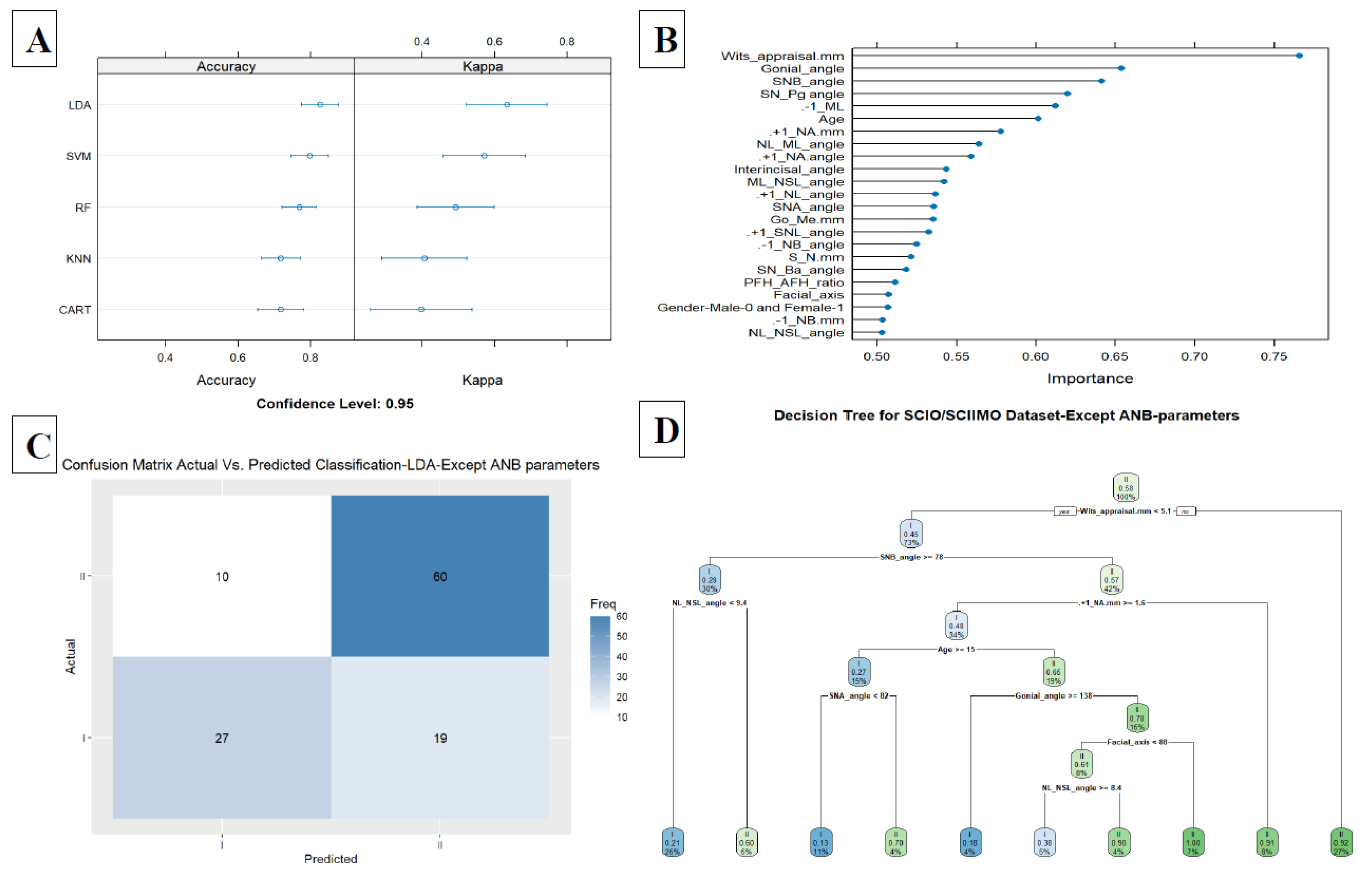
Table 1.
A- Hierarchical clustering results summary according to their skeletal classification. Summary of hierarchical Ward clustering results when using all variables. It represents the number of patients in each cluster and their classification (separate clustering for each skeletal classification class I and II). B. Hierarchical clustering analysis for skeletal class I patients. The cephalometric parameters, descriptive statistics, mean, and standard deviation (SD) for each cluster, when skeletal class I patients. In addition, the tables present the ANOVA significance levels of the comparisons between the three clusters in each malocclusion group (NS- not significant, *<0.05, **<0.01, and ***<0.001). C. Hierarchical clustering analysis for skeletal class I patients with gender effect. The cephalometric parameters, descriptive statistics, mean, and standard deviation (SD) for each cluster, including skeletal class I), but with each gender separately. In addition, the tables present the ANOVA significance levels of the comparisons between the three clusters in each malocclusion group (NS- not significant, *<0.05, **<0.01, and ***<0.001). D. Hierarchical clustering analysis for skeletal class II patients. The cephalometric parameters, descriptive statistics, mean, and standard deviation (SD) for each cluster, when including skeletal class II). In addition, the tables present the ANOVA significance levels of the comparisons between the three clusters in each malocclusion group (NS- not significant, *<0.05, **<0.01, and ***<0.001). E. Hierarchical clustering analysis for skeletal class II patients with gender effect. The cephalometric parameters, descriptive statistics, mean, and standard deviation (SD) for each cluster, including the skeletal class II patients, but with each gender separately. In addition, the tables present the ANOVA significance levels of the comparisons between the three clusters in each malocclusion group (NS- not significant, *<0.05, **<0.01, and ***<0.001).
| Parameters included |
Cluster |
Class Calculated ANB |
|
Class Calculated ANB |
|
| |
|
I |
|
II |
|
| All |
1 |
75 |
|
125 |
|
| 2 |
54 |
|
62 |
|
| 3 |
27 |
|
49 |
|
| Total |
156 |
|
236 |
|
| |
|
|
|
|
|
| Males |
1 |
20 |
|
20 |
|
| 2 |
18 |
|
27 |
|
| 3 |
15 |
|
31 |
|
| Total |
53 |
|
78 |
|
| |
|
|
|
|
| Females |
1 |
25 |
|
58 |
|
| 2 |
50 |
|
75 |
|
| 3 |
28 |
|
25 |
|
| Total |
103 |
|
158 |
|
| B |
| Parameter |
Class I Malocclusion |
| |
Cluster 1 |
Cluster 2 |
Cluster 3 |
|
| |
Mean |
SD |
Mean |
SD |
Mean |
SD |
Sig ANOVA |
| Age |
17.95 |
4.84 |
19.73 |
9.01 |
18.89 |
7.30 |
NS |
| NL-ML angle [°] |
32.27 |
6.07 |
29.21 |
4.13 |
24.66 |
5.35 |
*** |
| NL-NSL angle [°] |
8.27 |
3.54 |
8.32 |
2.68 |
5.21 |
2.70 |
*** |
| PFH/AFH (%) |
62.93 |
4.85 |
64.54 |
3.40 |
70.32 |
4.05 |
*** |
| Gonial angle [°] |
135.33 |
7.82 |
131.86 |
4.64 |
127.57 |
7.59 |
*** |
| Facial axis |
86.62 |
4.17 |
88.42 |
3.88 |
91.86 |
4.40 |
*** |
| SNA angle [°] |
82.29 |
3.67 |
80.89 |
2.98 |
86.64 |
3.42 |
*** |
| SNB angle [°] |
76.92 |
3.25 |
77.56 |
3.30 |
81.66 |
2.73 |
*** |
| ANB angle [°] |
5.37 |
1.62 |
3.32 |
1.36 |
4.97 |
2.05 |
** |
| ANBind [°] |
5.86 |
1.48 |
4.73 |
0.97 |
5.45 |
1.60 |
* |
| Calculated_ANB (ANB – ANBind) [°] |
-0.49 |
1.01 |
-1.41 |
1.49 |
-0.48 |
1.30 |
NS |
| SN-Ba angle [°] |
129.47 |
5.95 |
130.24 |
4.95 |
124.69 |
5.24 |
** |
| SN-Pg angle [°] |
77.65 |
3.60 |
78.14 |
3.45 |
82.34 |
2.97 |
*** |
| S-N (mm) |
60.75 |
7.63 |
63.05 |
6.31 |
66.74 |
8.01 |
*** |
| Go-Me (mm) |
57.83 |
6.59 |
60.18 |
5.54 |
62.96 |
7.00 |
*** |
| Wits appraisal (mm) |
1.62 |
2.27 |
0.88 |
2.69 |
3.25 |
1.97 |
NS |
| ML-NSL angle [°] |
40.22 |
6.29 |
37.29 |
4.16 |
29.28 |
6.60 |
*** |
| +1/NL angle [°] |
110.76 |
5.20 |
116.63 |
4.08 |
119.09 |
4.85 |
*** |
| +1/SNL angle [°] |
102.44 |
6.59 |
108.41 |
4.61 |
113.99 |
5.60 |
*** |
| +1/NA angle [°] |
20.29 |
5.44 |
27.33 |
4.23 |
27.69 |
6.17 |
*** |
| +1/NA (mm) |
2.56 |
1.63 |
4.64 |
1.87 |
5.21 |
2.57 |
*** |
| -1/ML (anatomic) |
89.76 |
6.53 |
92.69 |
6.23 |
100.18 |
5.87 |
*** |
| -1/NB angle [°] |
26.71 |
6.86 |
27.66 |
5.68 |
31.70 |
5.62 |
** |
| -1/NB (mm) |
5.35 |
2.32 |
5.07 |
2.06 |
6.75 |
2.52 |
* |
| Interincisal angle [°] |
128.52 |
10.42 |
121.75 |
7.37 |
116.04 |
6.66 |
*** |
| C |
| |
Class I Males |
|
Class I Females |
|
| Cluster |
1 |
2 |
3 |
Sig ANOVA |
1 |
2 |
3 |
Sig ANOVA |
| |
Mean |
SD |
Mean |
SD |
Mean |
SD |
|
Mean |
SD |
Mean |
SD |
Mean |
SD |
|
| Age |
16.01 |
4.04 |
17.73 |
6.48 |
17.59 |
3.11 |
NS |
16.63 |
4.76 |
21.22 |
9.48 |
19.35 |
5.45 |
NS |
| NL-ML angle [°] |
31.72 |
5.40 |
25.45 |
5.85 |
30.57 |
5.74 |
NS |
36.34 |
4.66 |
27.65 |
4.41 |
29.34 |
5.32 |
*** |
| NL-NSL angle [°] |
8.72 |
3.23 |
5.11 |
3.23 |
6.55 |
3.08 |
* |
7.79 |
3.72 |
9.09 |
2.76 |
7.02 |
2.88 |
NS |
| PFH/AFH (%) |
63.58 |
4.11 |
69.72 |
4.73 |
65.69 |
3.31 |
NS |
60.66 |
5.77 |
64.91 |
3.50 |
65.34 |
5.08 |
*** |
| Gonial angle [°] |
135.85 |
6.95 |
128.03 |
7.59 |
132.75 |
6.86 |
NS |
139.99 |
5.59 |
130.45 |
6.37 |
131.40 |
5.84 |
*** |
| Facial axis |
87.17 |
4.80 |
91.83 |
4.87 |
86.88 |
4.91 |
NS |
84.83 |
4.01 |
88.89 |
2.94 |
88.82 |
4.50 |
*** |
| SNA angle [°] |
79.68 |
3.28 |
85.22 |
3.50 |
85.58 |
3.06 |
*** |
82.49 |
3.31 |
81.23 |
3.61 |
83.72 |
3.73 |
NS |
| SNB angle [°] |
75.77 |
2.95 |
81.39 |
3.02 |
78.99 |
2.44 |
** |
76.61 |
3.81 |
77.41 |
3.40 |
78.98 |
3.20 |
* |
| ANB angle [°] |
3.94 |
1.30 |
3.83 |
1.91 |
6.59 |
1.30 |
*** |
5.89 |
1.30 |
3.82 |
1.59 |
4.70 |
1.96 |
* |
| ANBind [°] |
4.79 |
1.40 |
5.01 |
1.63 |
6.50 |
1.21 |
** |
6.64 |
0.65 |
4.67 |
1.19 |
5.67 |
1.22 |
* |
Calculated_ANB
(ANB – ANBind) [°] |
-0.86 |
1.05 |
-1.18 |
1.70 |
0.09 |
0.79 |
NS |
-0.75 |
1.03 |
-0.86 |
1.53 |
-0.97 |
1.12 |
NS |
| SN-Ba angle [°] |
130.94 |
5.10 |
125.87 |
6.01 |
124.83 |
5.79 |
** |
129.02 |
5.40 |
131.29 |
5.73 |
127.26 |
4.25 |
NS |
| SN-Pg angle [°] |
76.67 |
2.95 |
82.08 |
3.52 |
79.59 |
3.04 |
* |
76.90 |
4.29 |
78.14 |
3.40 |
79.74 |
3.54 |
** |
| S-N (mm) |
60.52 |
8.82 |
68.34 |
9.05 |
67.02 |
8.96 |
* |
57.64 |
3.56 |
62.10 |
5.81 |
63.25 |
6.80 |
*** |
| Go-Me (mm) |
58.27 |
5.13 |
63.22 |
7.85 |
62.13 |
9.72 |
NS |
54.66 |
3.79 |
59.65 |
5.14 |
60.79 |
6.54 |
*** |
| Wits appraisal (mm) |
0.62 |
2.73 |
2.90 |
2.50 |
2.92 |
1.61 |
** |
1.36 |
2.53 |
1.28 |
2.59 |
1.79 |
2.07 |
NS |
| ML-NSL angle [°] |
39.56 |
6.06 |
30.46 |
5.31 |
37.13 |
4.92 |
NS |
43.87 |
6.73 |
36.52 |
4.08 |
35.75 |
8.19 |
*** |
| +1/NL angle [°] |
114.31 |
3.92 |
119.83 |
3.82 |
107.61 |
6.05 |
** |
110.62 |
4.55 |
113.14 |
4.41 |
119.31 |
4.35 |
*** |
| +1/SNL angle [°] |
105.69 |
5.21 |
114.90 |
4.58 |
101.19 |
7.32 |
NS |
102.84 |
6.67 |
103.77 |
4.96 |
112.69 |
5.17 |
*** |
| +1/NA angle [°] |
25.91 |
3.91 |
29.68 |
3.83 |
15.52 |
5.85 |
*** |
20.56 |
4.59 |
22.68 |
4.78 |
29.02 |
4.93 |
*** |
| +1/NA (mm) |
4.02 |
1.73 |
5.74 |
2.14 |
1.09 |
1.67 |
** |
2.81 |
1.21 |
3.20 |
1.55 |
5.47 |
2.22 |
*** |
| -1/ML (anatomic) |
90.16 |
6.97 |
97.39 |
8.07 |
92.79 |
6.14 |
NS |
87.31 |
5.94 |
91.36 |
5.89 |
97.97 |
6.22 |
*** |
| -1/NB angle [°] |
25.94 |
7.14 |
29.34 |
6.60 |
28.73 |
6.97 |
NS |
28.05 |
6.08 |
25.15 |
4.52 |
32.71 |
6.34 |
** |
| -1/NB (mm) |
4.93 |
2.32 |
6.23 |
2.89 |
5.46 |
2.38 |
NS |
6.09 |
1.50 |
4.45 |
1.89 |
6.77 |
2.46 |
NS |
| Interincisal angle [°] |
125.58 |
10.60 |
117.24 |
8.38 |
130.14 |
12.03 |
NS |
126.23 |
6.98 |
128.44 |
7.47 |
114.08 |
6.15 |
*** |
| D |
| Parameter |
Class II Malocclusion |
| |
Cluster 1 |
Cluster 2 |
Cluster 3 |
|
| |
Mean |
SD |
Mean |
SD |
Mean |
SD |
Sig ANOVA |
| Age |
17.59 |
7.20 |
15.50 |
3.83 |
18.20 |
7.04 |
NS |
| NL-ML angle [°] |
30.25 |
5.68 |
24.15 |
4.91 |
31.49 |
7.13 |
NS |
| NL-NSL angle [°] |
7.82 |
4.16 |
7.89 |
2.83 |
9.15 |
3.40 |
NS |
| PFH/AFH (%) |
64.01 |
4.54 |
68.18 |
4.58 |
62.56 |
4.88 |
NS |
| Gonial angle [°] |
130.62 |
7.29 |
124.60 |
6.44 |
131.42 |
6.27 |
NS |
| Facial axis |
87.95 |
3.98 |
90.22 |
3.77 |
84.13 |
4.57 |
*** |
| SNA angle [°] |
83.42 |
3.56 |
82.12 |
4.05 |
81.67 |
3.42 |
** |
| SNB angle [°] |
76.21 |
2.85 |
77.22 |
3.34 |
72.21 |
9.84 |
*** |
| ANB angle [°] |
7.17 |
1.93 |
4.90 |
2.02 |
8.16 |
1.94 |
NS |
| ANBind [°] |
5.76 |
1.45 |
4.13 |
1.25 |
5.63 |
1.73 |
* |
| Calculated_ANB (ANB – ANBind) [°] |
1.40 |
1.34 |
0.77 |
1.63 |
2.53 |
1.15 |
*** |
| SN-Ba angle [°] |
129.79 |
5.63 |
129.89 |
5.04 |
130.18 |
5.22 |
NS |
| SN-Pg angle [°] |
76.95 |
2.95 |
78.72 |
3.28 |
73.65 |
3.24 |
*** |
| S-N (mm) |
64.09 |
7.80 |
60.68 |
6.39 |
61.58 |
5.89 |
** |
| Go-Me (mm) |
59.64 |
6.51 |
59.03 |
4.35 |
55.87 |
5.10 |
*** |
| Wits appraisal (mm) |
5.09 |
3.44 |
3.09 |
2.90 |
5.46 |
3.06 |
NS |
| ML-NSL angle [°] |
37.91 |
5.72 |
32.01 |
5.45 |
40.65 |
6.74 |
NS |
| +1/NL angle [°] |
117.33 |
5.76 |
109.92 |
5.38 |
105.64 |
5.90 |
*** |
| +1/SNL angle [°] |
109.91 |
5.87 |
102.15 |
5.63 |
96.49 |
6.25 |
*** |
| +1/NA angle [°] |
26.65 |
6.04 |
20.34 |
6.81 |
14.86 |
6.46 |
*** |
| +1/NA (mm) |
4.35 |
2.09 |
2.05 |
1.96 |
1.21 |
1.73 |
*** |
| -1/ML (anatomic) |
96.30 |
7.24 |
92.48 |
8.35 |
96.69 |
7.03 |
NS |
| -1/NB angle [°] |
30.61 |
5.64 |
21.99 |
7.29 |
30.94 |
6.45 |
NS |
| -1/NB (mm) |
6.43 |
2.14 |
3.14 |
1.64 |
6.08 |
2.54 |
** |
| Interincisal angle [°] |
116.10 |
7.28 |
133.34 |
8.85 |
126.15 |
8.73 |
*** |
| E |
| |
Class II Males |
|
Class II Females |
|
| Cluster |
1 |
2 |
3 |
Sig ANOVA |
1 |
2 |
3 |
Sig ANOVA |
| |
Mean |
SD |
Mean |
SD |
Mean |
SD |
|
Mean |
SD |
Mean |
SD |
Mean |
SD |
|
| Age |
12.90 |
2.20 |
17.58 |
7.09 |
16.98 |
6.39 |
* |
15.88 |
5.11 |
18.76 |
7.71 |
18.56 |
5.53 |
* |
| NL-ML angle [°] |
30.66 |
4.50 |
23.91 |
5.06 |
31.93 |
6.56 |
NS |
27.73 |
4.80 |
32.35 |
5.73 |
21.59 |
4.34 |
* |
| NL-NSL angle [°] |
7.78 |
3.04 |
6.67 |
3.04 |
8.16 |
3.40 |
NS |
9.28 |
2.50 |
8.50 |
4.89 |
6.03 |
2.21 |
** |
| PFH/AFH (%) |
62.79 |
2.75 |
70.12 |
3.29 |
62.72 |
3.62 |
NS |
64.62 |
3.60 |
62.03 |
4.00 |
72.00 |
4.18 |
*** |
| Gonial angle [°] |
131.55 |
5.80 |
125.35 |
8.20 |
131.92 |
6.07 |
NS |
128.24 |
6.75 |
132.11 |
6.44 |
121.64 |
5.80 |
* |
| Facial axis |
89.40 |
3.37 |
90.53 |
3.88 |
85.44 |
4.43 |
*** |
87.27 |
3.20 |
86.29 |
4.83 |
91.78 |
3.78 |
** |
| SNA angle [°] |
79.16 |
2.73 |
84.61 |
3.45 |
83.37 |
3.23 |
*** |
80.69 |
2.58 |
83.19 |
3.72 |
85.99 |
2.99 |
*** |
| SNB angle [°] |
71.62 |
15.21 |
78.30 |
2.19 |
75.17 |
3.15 |
NS |
74.81 |
2.53 |
75.18 |
3.18 |
79.93 |
2.38 |
*** |
| ANB angle [°] |
4.35 |
2.10 |
6.33 |
1.94 |
8.19 |
1.46 |
*** |
5.87 |
1.92 |
7.95 |
1.98 |
6.03 |
2.28 |
NS |
| ANBind [°] |
4.19 |
1.28 |
4.81 |
1.83 |
6.21 |
1.50 |
*** |
4.54 |
1.24 |
6.18 |
1.42 |
4.75 |
1.29 |
* |
Calculated_ANB
(ANB – ANBind) [°] |
0.16 |
1.86 |
1.51 |
0.90 |
1.98 |
1.11 |
*** |
1.32 |
1.56 |
1.78 |
1.46 |
1.28 |
1.61 |
NS |
| SN-Ba angle [°] |
132.49 |
5.93 |
128.94 |
3.43 |
129.23 |
5.55 |
* |
130.73 |
5.69 |
129.79 |
5.57 |
128.06 |
4.36 |
* |
| SN-Pg angle [°] |
75.47 |
2.17 |
79.43 |
2.29 |
75.35 |
3.55 |
NS |
75.93 |
2.71 |
75.83 |
3.50 |
81.08 |
2.64 |
*** |
| S-N (mm) |
65.31 |
8.55 |
62.81 |
6.49 |
66.27 |
7.58 |
NS |
60.15 |
3.80 |
63.19 |
7.69 |
60.27 |
8.57 |
NS |
| Go-Me (mm) |
59.86 |
8.26 |
58.31 |
6.03 |
61.29 |
6.31 |
NS |
56.70 |
4.39 |
58.63 |
6.16 |
59.82 |
3.67 |
** |
| Wits appraisal (mm) |
2.84 |
2.96 |
4.81 |
2.67 |
5.34 |
3.32 |
** |
3.68 |
3.47 |
5.48 |
3.28 |
4.75 |
3.45 |
* |
| ML-NSL angle [°] |
38.49 |
3.76 |
30.51 |
4.27 |
40.09 |
5.66 |
NS |
37.06 |
4.77 |
40.43 |
5.74 |
27.89 |
4.50 |
*** |
| +1/NL angle [°] |
113.42 |
7.25 |
114.98 |
6.84 |
109.57 |
8.16 |
* |
108.31 |
5.22 |
115.62 |
6.25 |
117.43 |
8.46 |
*** |
| +1/SNL angle [°] |
105.70 |
6.99 |
108.34 |
7.63 |
101.74 |
9.00 |
NS |
99.11 |
5.63 |
107.67 |
6.27 |
111.38 |
7.50 |
*** |
| +1/NA angle [°] |
26.79 |
7.19 |
23.70 |
6.46 |
18.08 |
7.53 |
*** |
18.87 |
6.56 |
24.65 |
7.44 |
25.60 |
9.08 |
*** |
| +1/NA (mm) |
4.94 |
2.59 |
3.00 |
2.31 |
2.35 |
2.31 |
*** |
1.74 |
1.72 |
3.81 |
2.28 |
3.65 |
2.42 |
*** |
| -1/ML (anatomic) |
90.43 |
4.57 |
98.56 |
6.57 |
98.90 |
8.38 |
*** |
91.25 |
6.76 |
95.56 |
6.81 |
100.52 |
7.58 |
*** |
| -1/NB angle [°] |
23.85 |
4.22 |
27.64 |
8.33 |
34.23 |
6.57 |
*** |
23.34 |
6.38 |
31.40 |
5.14 |
28.54 |
7.39 |
*** |
| -1/NB (mm) |
4.25 |
2.07 |
4.73 |
1.98 |
7.80 |
2.13 |
*** |
3.53 |
1.56 |
6.86 |
2.10 |
4.92 |
2.42 |
*** |
| Interincisal angle [°] |
125.30 |
7.49 |
122.58 |
12.99 |
119.85 |
8.68 |
NS |
132.57 |
8.35 |
116.48 |
7.73 |
120.19 |
10.89 |
*** |
Table 2.
Stepwise Forward Machine Learning Models. Stepwise Forward Machine Learning Models, including General model, Model 1, Model 2, and Model 3: These rows represent different models used for prediction, potentially containing various combinations of the cephalometric parameters. The general model included all parameters. In models 1-3, the sign (-) indicates that the parameter was not included, while (+) indicates that the parameter is included.
| |
ANB |
Wits appraisal |
-1/NB angle |
Gonial Angle |
Best Model |
Accuracy |
Kappa |
ROC curve |
Sensitivity |
Specificity |
| General model |
RF, CART |
0.87 |
0.74 |
RF-0.92,
CART-0.90 |
RF-0.92,
CART-0.94 |
RF-0.83,
CART-0.82 |
| Model 1 |
(+) |
(-) |
(-) |
(-) |
LDA |
0.75 |
0.47 |
0.79 |
0.59 |
0.86 |
| Model 2 |
(+) |
(+) |
(-) |
(-) |
KNN |
0.78 |
0.56 |
0.82 |
0.80 |
0.76 |
| Model 3 |
All variables except ANB, ANBind, and Calculated_ANB |
LDA |
0.82
|
0.63
|
0.88 |
0.75 |
0.87 |
|
Disclaimer/Publisher’s Note: The statements, opinions and data contained in all publications are solely those of the individual author(s) and contributor(s) and not of MDPI and/or the editor(s). MDPI and/or the editor(s) disclaim responsibility for any injury to people or property resulting from any ideas, methods, instructions or products referred to in the content. |
© 2024 by the authors. Licensee MDPI, Basel, Switzerland. This article is an open access article distributed under the terms and conditions of the Creative Commons Attribution (CC BY) license (http://creativecommons.org/licenses/by/4.0/).