Thermodynamic Theory of Gravity and Buoyancy

1. Introduction

In physics, it is generally believed that there are four elementary forces

• Newton’s gravity force [1,2], e.g., the free fall of a steel ball towards the earth;
• Electromagnetic force [3,4], e.g., Coulomb force;
• Strong force [5,6], e.g., interaction of protons and neutrons;
• Weak force [7,8].

The latter three forces have been unified [9,10,11,12]. Whether gravity is an independent elementary force has not yet been resolved [2,13,14] in the community of physics. In contrast to quantum gravity theory [15,16,17,18], we here shed light on gravitational force from the perspective of thermodynamics, where the total energy of a closed system must be non-increasing.

It is well known that a steel particle falls in the air towards the earth with an acceleration constant of $g\approx 9.8$ m²/s (Figure 1a). In another scenario, the steel particle can also fall down freely in the water with an acceleration constant $g^{*}$ differing from g. In conventional theories, the acceleration constant of a falling particle in water differing from g is attributed to two forces

$$\mathrm{gravity}\text{:}{\rho }_{p}g{V}_p;\mathrm{and}\mathrm{buoyancy}\text{:}{\rho }_{p}g{V}_p.$$

(1)

Here, ${\rho }_p$ and ${\rho }_f$ represent the density of the particle and the surrounding, respectively; $V_p$ denotes the volume of the particle. Drag force is not considered, since at the linear acceleration stage, water can be considered as an inviscid fluid; in other words, the entropy increase takes a much longer time than the inertial acceleration. According to Newton’s law, we have a simple force balance between inertial force, gravity, and buoyancy as

$$\begin{array}{c}\hfill \mathrm{Inertial}\mathrm{force}=\mathrm{Gravity}+\mathrm{Buoyancy}\iff {\rho }_p{V}_p{g}^{*}={\rho }_{p}g{V}_p-{\rho }_{f}g{V}_p.\end{array}$$

A brief calculation shows that the acceleration of a falling particle in water according to conventional theories is

$$g^{*}=(1-{\rho }_f/{\rho }_p)g,$$

(2)

which significantly deviates from existing experiments [19,20]. From the opinion of the current authors, the reason for the conflict between existing theories and experiments is the unclear physical origin of gravity and buoyancy.

In this work, we show that Newton’s second law is actually derived from microscopic potential energy. Our derivation involves reformulating kinetic energy in a way that differs from classical theories, leading to a generalized formulation for calculating the acceleration of a particle in an inviscid fluid. We also quantitatively compare our theory of gravity with experimental data for the free fall of a steel particle in water.

2. Origin of Newton’s Law and Energy Dissipation

We consider the motion of a solid particle, like a steel ball, in the surrounding of air or water. The system is placed in a closed domain $\mathsf{\Omega }$ without external forces and consists of the microscopic potential energy $\mathcal{P}$ and the macroscopic kinetic energy $\mathcal{K}$

$$\mathcal{E}=\mathcal{P}+\mathcal{K}.$$

(3)

The energy minimization principle requires that for a closed system, the total energy of the system must be non-increasing with time t, namely

$${\displaystyle \frac{\mathrm{d}\mathcal{E}}{\mathrm{d}t}}={\displaystyle \frac{\mathrm{d}\mathcal{P}}{\mathrm{d}t}}+{\displaystyle \frac{\mathrm{d}\mathcal{K}}{\mathrm{d}t}}\le 0.$$

(4)

The time derivative of the potential energy reads

$${\displaystyle \frac{\mathrm{d}\mathcal{P}}{\mathrm{d}t}}={\displaystyle \frac{\mathrm{d}}{\mathrm{d}t}}{\int }_{\mathsf{\Omega }}p\mathrm{d}\mathsf{\Omega }={\int }_{\mathsf{\Omega }}{\displaystyle \frac{\mathrm{d}p}{d\mathbf{r}}}·{\displaystyle \frac{\mathrm{d}\mathbf{r}}{\mathrm{d}t}}\mathrm{d}\mathsf{\Omega }={\int }_{\mathsf{\Omega }}\nabla p·\mathbf{u}\mathrm{d}\mathsf{\Omega },$$

(5)

where p is the density of the thermodynamic potential energy and $\mathbf{u}$ depicts the local fluid velocity according to

$$\mathbf{u}={\displaystyle \frac{\mathrm{d}\mathbf{r}}{\mathrm{d}t}}.$$

(6)

The microscopic potential energy p, also known as the thermodynamic pressure, is due to the motion, collision, and electromagnetic interaction of molecules and atoms at the microscopic scale. An explicit formulation of p is [21,22]

$$-p=f-\sum _{i=1}^K{\mu }_i{c}_i,$$

(7)

which is consistent with the Landau potential. Here, f denotes the free energy, ${\mu }_i$ and $c_i$ depict the chemical potential and composition of component i, respectively; K stands for the number of the components in the system. A specialized discussion of p including chemical free energy, electrostatic energy, etc, has been presented in [23].

A key controversial point is the formulation of the kinetic energy. We formulate the kinetic energy in the classic theory and in the present work as

$$\begin{array}{cc}\hfill & \mathrm{Classic}\mathrm{theory}\text{:}\tilde{\mathcal{K}}={\int }_{\mathsf{\Omega }}\rho {\mathbf{u}}^2\mathrm{d}\mathsf{\Omega };\hfill \end{array}$$

(8)

$$\begin{array}{cc}\hfill & \mathrm{Present}\mathrm{theory}\text{:}\mathcal{K}={\int }_{\mathsf{\Omega }}\mathit{\theta }·\mathbf{u}\mathrm{d}\mathsf{\Omega };\mathit{\theta }=\rho \mathbf{u},\hfill \end{array}$$

(9)

where $\rho$ represents the local density and $\mathit{\theta }$ is the linear momentum. The total time derivative of the kinetic energy in the conventional and current theories reads

$$\begin{array}{cc}\hfill & \mathrm{Classic}\mathrm{theory}\text{:}{\displaystyle \frac{\mathrm{d}\tilde{\mathcal{K}}}{\mathrm{d}t}}={\int }_{\mathsf{\Omega }}{\displaystyle \frac{\mathrm{d}\rho }{\mathrm{d}t}}{\mathbf{u}}^2+2\rho \mathbf{u}·{\displaystyle \frac{\mathrm{d}\mathbf{u}}{\mathrm{d}t}}\mathrm{d}\mathsf{\Omega };\hfill \end{array}$$

(10)

$$\begin{array}{cc}\hfill & \mathrm{Present}\mathrm{theory}\text{:}{\displaystyle \frac{\mathrm{d}\mathcal{K}}{\mathrm{d}t}}={\int }_{\mathsf{\Omega }}{\displaystyle \frac{\mathrm{d}\mathit{\theta }}{\mathrm{d}t}}·\mathbf{u}+\mathit{\theta }·{\displaystyle \frac{\mathrm{d}\mathbf{u}}{\mathrm{d}t}}\mathrm{d}\mathsf{\Omega }.\hfill \end{array}$$

(11)

A combination of Eq. (10) and Eq. (11) with Eq. (5) leads to the total time derivative of the system energy in the classic theory and in the present work as

$$\begin{array}{cc}\hfill \mathrm{Classic}& \mathrm{theory}\text{:}{\displaystyle \frac{\mathrm{d}\mathcal{E}}{\mathrm{d}t}}={\displaystyle \frac{\mathrm{d}\tilde{\mathcal{K}}}{\mathrm{d}t}}+{\displaystyle \frac{\mathrm{d}\mathcal{P}}{\mathrm{d}t}}\hfill \\ \hfill & ={\int }_{\mathsf{\Omega }}{\displaystyle \frac{\mathrm{d}\rho }{\mathrm{d}t}}{\mathbf{u}}^2+2\rho \mathbf{u}·{\displaystyle \frac{\mathrm{d}\mathbf{u}}{\mathrm{d}t}}+\nabla p·\mathbf{u}\mathrm{d}\mathsf{\Omega };\hfill \end{array}$$

(12)

$$\begin{array}{cc}\hfill \mathrm{Present}& \mathrm{theory}\text{:}{\displaystyle \frac{\mathrm{d}\mathcal{E}}{\mathrm{d}t}}={\displaystyle \frac{\mathrm{d}\mathcal{K}}{\mathrm{d}t}}+{\displaystyle \frac{\mathrm{d}\mathcal{P}}{\mathrm{d}t}}\hfill \\ \hfill & ={\int }_{\mathsf{\Omega }}\underset{\mathrm{I}}{\underbrace{\left(\nabla p+{\displaystyle \frac{\mathrm{d}\mathit{\theta }}{\mathrm{d}t}}\right)}}·\mathbf{u}+\underset{\mathrm{II}}{\underbrace{\mathit{\theta }·{\displaystyle \frac{\mathrm{d}\mathbf{u}}{\mathrm{d}t}}}}\mathrm{d}\mathsf{\Omega }.\hfill \end{array}$$

(13)

In Eq. (13), we have identified two parts, I and II, for the time evolution of the total energy. The first part, I is responsible for the exchange of the microscopic potential energy with the momentum; the microscopic potential energy corresponds to a conservative force $-\nabla p$. The second part, II is responsible for the dissipation of the velocity with the dissipative force $\propto \mathit{\theta }$.

$$\begin{array}{cc}\hfill & \mathrm{I},\mathrm{momentum}\mathrm{balance}\text{:}{\displaystyle \frac{\mathrm{d}\mathit{\theta }}{\mathrm{d}t}}=-\nabla p;\hfill \end{array}$$

(14)

$$\begin{array}{cc}\hfill & \mathrm{II},\mathrm{velocity}\mathrm{dissipation}\text{:}{\displaystyle \frac{\mathrm{d}\mathbf{u}}{\mathrm{d}t}}=-\tau \mathit{\theta }.\hfill \end{array}$$

(15)

The first equation is nothing but the momentum balance. By expanding the total time derivative

$${\displaystyle \frac{\mathrm{d}\mathit{\theta }}{\mathrm{d}t}}={\displaystyle \frac{\mathrm{d}\left(\rho \mathbf{u}\right)}{\mathrm{d}t}}=\rho {\displaystyle \frac{\mathrm{d}\mathbf{u}}{\mathrm{d}t}}+\mathbf{u}{\displaystyle \frac{\mathrm{d}\rho }{\mathrm{d}t}}$$

(16)

and considering the incompressible condition $\mathrm{d}\rho /\mathrm{d}t=0$, we obtain Newton’s law

$$\rho {\displaystyle \frac{\mathrm{d}\mathbf{u}}{\mathrm{d}t}}=-\nabla p,$$

(17)

which is also consistent with Euler’s equation. The stress tensor, such as Korteweg, Maxwell, and Cauchy stress tensor can also appear on the right hand side of Eq. (17) if we consider the contribution of chemical free energy, electrostatic potential energy, and elastic energy to $\mathcal{E}$ in Eq. (3); see the derivations in [23]. The above derivation reveals the thermodynamic origin of Newton’s law as well as the momentum balance. It should be emphasized that the potential energy p corresponds to the conservative force $-\nabla p$. Non-conservative forces, like viscous stress, have no corresponding potential energy and should not be added in the momentum evolution. The non-conservative force can only dissipate the velocity, as stated in Eq. (15), which decreases the kinetic energy. The dissipation coefficient $\tau$ is known as the drag coefficient. In fact, Eq. (15) is consistent with the classic Langevin equation [24] for the velocity dissipation if we define a new coefficient $\xi :=\tau \rho$, namely

$${\displaystyle \frac{\mathrm{d}\mathbf{u}}{\mathrm{d}t}}=-\tau \mathit{\theta }=-\tau \rho \mathbf{u}=-\xi \mathbf{u}.$$

(18)

We note that the classical theory, as given by Eq. (10), cannot account for the momentum balance. With the new formulation of kinetic energy, we have successfully derived the momentum balance equation, which addresses the exchange between kinetic and potential energy. We have also revealed that Newton’s law is intrinsically caused by the thermodynamic potential energy, which is caused by the random motion, electromagnetic interaction, collision of molecules/atoms at the microscopic scale. This concept is consistent with a recent hypothesis of Verlinde that the origin of Newton’s law is the microscopic entropy [2]. Note that the second law of Newton relating the conservative force $\mathit{F}$, mass m, and acceleration $\mathit{a}$,

$$\mathit{F}=m\mathit{a}$$

(19)

is only true when $\mathrm{d}m/\mathrm{d}t=0$ or $\mathrm{d}\rho /\mathrm{d}t=0$ . When there is an evolution of the density, the second law of Newton has to be amended by the momentum balance equation. We stress again that the dissipative non-conservative force cannot be included in the momentum balance; only the conservative force is responsible for the momentum equation.

Note that the dissipation formulation for the velocity $\mathbf{u}$ can be diverse. While the formulation of the momentum balance is unique, there is no such a unique formulation for the velocity dissipation. From the part II in Eq. (13), we may formulate another dissipation for the velocity according to the dissipation-conservation theorem as (see Appendix)

$${\displaystyle \frac{\mathrm{d}\mathbf{u}}{\mathrm{d}t}}=\nabla ·{\tau }_0\mathit{\theta }.$$

(20)

When defining the dissipation coefficient ${\tau }_0=\mu /{\rho }^2$ in terms of viscosity $\mu$ and assuming $\rho =\mathrm{constant}$, we obtain the Newton dissipation as

$$\rho {\displaystyle \frac{\mathrm{d}\mathbf{u}}{\mathrm{d}t}}=\nabla ·\mu \nabla \mathbf{u}.$$

(21)

There are many other types of non-linear dissipation that are beyond the scope of the present work.

3. Origin of Gravity and Buoyancy

Next, we consider the free fall of a steel particle in the surrounding on top of the earth. The surrounding could be air or water. The momentum balance equation reads

$${\displaystyle \frac{\mathrm{d}\left(\rho \mathbf{u}\right)}{\mathrm{d}t}}=-\nabla p.$$

(22)

In contrast to the conventional theory that an additional gravity force $\rho g$ is added to the above equation, we insist that an intrinsic acceleration ${\displaystyle \frac{\mathrm{d}\mathbf{u}}{\mathrm{d}t}}$ will be obtained by considering the thermodynamic pressure arising from the density difference.

When the particle falls down freely, it is sufficient to consider the momentum evolution in the falling-dimension, say x-direction (Figure 1a), to calculate the acceleration. The velocity in the x-direction is denoted as u. For incompressible fluids with $\mathrm{d}\rho /\mathrm{d}t=0$ (for compressible fluids and density evolution, see Ref. [25]), the momentum balance equation is rewritten as

$$\rho {\displaystyle \frac{\mathrm{d}u}{\mathrm{d}t}}=-{\displaystyle \frac{\mathrm{d}p}{\mathrm{d}x}}.$$

(23)

As sketched in Figure 1a, we choose the moving coordinate along with the particle and assume that the velocity decays from the particle through the surrounding to the surface of the earth as

$$u(t,x)=u_0\left(t\right)exp(-\mathsf{\ell }x).$$

(24)

At the surface of the particle, $x=0$, the velocity is $u_0$; far away from the particle $x=+\infty$, the velocity decays to zero. The characteristic length parameter ℓ is related to the average thickness of the boundary layer for the particle-surrounding system in the context of fluid dynamics [26]. We assume that the density decays from the particle (${\rho }_p$) to the surrounding (${\rho }_s$) over a distance $\lambda$ as

$$\rho \left(x\right)=({\rho }_p-{\rho }_s)e^{-\lambda x}+{\rho }_s,\lambda \ll \mathsf{\ell }.$$

(25)

Substituting Eq. (24) and Eq. (25) into Eq. (23) and integrating from the surface of the falling particle ($x=0$) to the surface of the earth $x=+\infty$, we obtain

$$\left[{\rho }_s+{\displaystyle \frac{\mathsf{\ell }}{\lambda +\mathsf{\ell }}}({\rho }_p-{\rho }_s)\right]{\displaystyle \frac{\mathrm{d}{u}_0}{\mathrm{d}t}}=\mathsf{\ell }[(p\left(0\right)-p(\infty )].$$

(26)

By using the condition $\lambda \ll \mathsf{\ell }$, Eq. (26) is rewritten as

$${\rho }_p{\displaystyle \frac{\mathrm{d}{u}_0}{\mathrm{d}t}}=\mathsf{\ell }[(p\left(0\right)-p(\infty )].$$

(27)

Here, $p\left(0\right)$ and $p(\infty )$ represent the thermodynamic pressure in the particle and in the surrounding, respectively. Note that in the inertial-dominated region, where the velocity increases linearly with time, it is reasonable to assume inviscid fluids, as the time scale of inertial acceleration is much shorter than that of dissipation. Note also that only conservative forces are responsible for the momentum evolution; non-conservative forces, such as viscosity, do not contribute to the momentum balance [25]. For inviscid fluids, the thermodynamic pressure can be expressed in terms of the sound speed c as: $p=c^2\rho$, according to sound wave theory [26]. In this way, we obtain a generalized formulation for the acceleration of the particle as follows:

$$a=\mathsf{\ell }(c_p^2-c_s^2{\rho }_s/{\rho }_p).$$

(28)

where the parameters $c_p$ and $c_s$ denote the speed of sound in the particle and in the surrounding phase, respectively.

4. Comparison with Experiments and Discussion

Next, we compare our results with classic theory of gravity and buoyancy as well as with experiments. In the classic theory, the inertial acceleration of the particle is a result of the gravity force ${\rho }_{p}g{V}_p$ plus the buoyancy force $-{\rho }_{s}g{V}_p$, namely

$${\rho }_p{V}_p{\displaystyle \frac{\mathrm{d}{u}_0}{\mathrm{d}t}}={\rho }_{p}g{V}_p-{\rho }_{f}g{V}_p,$$

(29)

where $V_p$ denotes the volume of the particle and $g=9.81$ m²/s stands for the gravity acceleration. According to Eq. (29), the acceleration in the classic theory is

$$g^{*}={\displaystyle \frac{\mathrm{d}{u}_0}{\mathrm{d}t}}=(1-{\rho }_s/{\rho }_p)g.$$

(30)

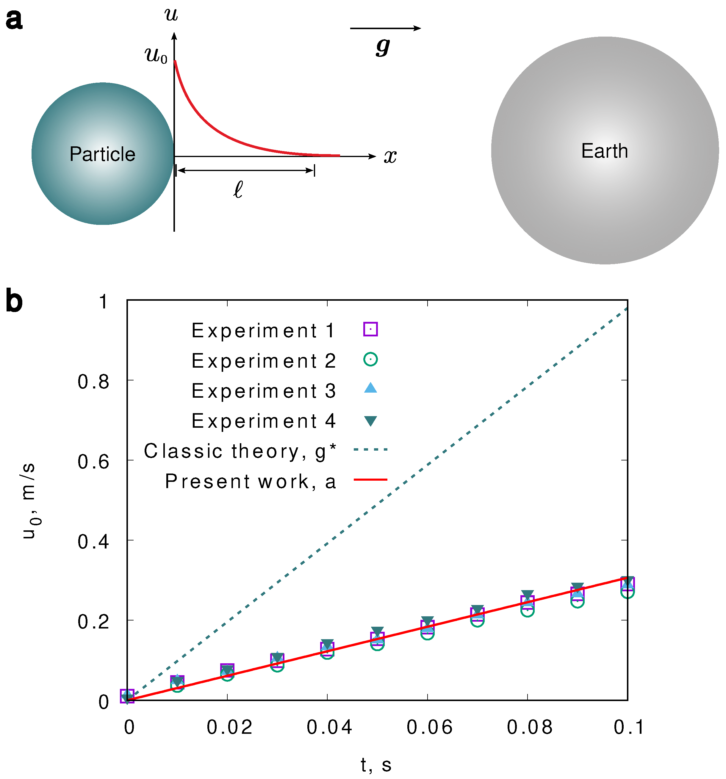
To show the problem of Eq. (30) according to classic theories, we consider the free fall of a steel particle in the water starting with a velocity 0 m/s. According to Eq. (30) with the physical parameters listed in Table 1, the acceleration constant is about 8.4 m/s²; this value significantly deviates from the experimental acceleration of around 3 m/s² for the falling steel ball in water (Figure 1b). The experimental value is well consistent with the present results according to Eq. (28). In our calculation, we set ${\mathsf{\ell }}_a{c}_{steel}^2=g=9.8$ m/s², where ${\mathsf{\ell }}_a$ denotes the boundary layer thickness of the steel ball in air and $c_{steel}$ stands for the sound speed in steel 1. According to the well-known boundary layer theory in fluid dynamics [26],

$$\mathsf{\ell }\propto \sqrt{\mu /\rho },$$

(31)

the boundary layer thickness in the water is

$${\mathsf{\ell }}_w=\sqrt{{\mu }_w{\rho }_a/{\mu }_a{\rho }_w}{\mathsf{\ell }}_a\approx {\mathsf{\ell }}_a/\sqrt{10}.$$

(32)

Here, ${\mu }_i$ and ${\rho }_i$ represent the viscosity and density of phase i (w: water, a: air), respectively. With the sound speed in water and the density ratio of water to steel, ${\rho }_s/{\rho }_p=0.13$, we obtain the acceleration of a steel ball in water as

$$a=3.05{\mathrm{m}/\mathrm{s}}^2.$$

(33)

Table 1. Density and viscosity [27] of steel, water, and air, and the sound speed [28].

Items/parameters	Density, $\mathit{\rho }$, kg/m3	Viscosity, $\mathit{\mu }$, Pa· s	Sound speed, c, m/s
Steel	7750	-	5000
Water	996	0.01	1500
Air	1	0.000018	340

Table 1. Density and viscosity [27] of steel, water, and air, and the sound speed [28].

Items/parameters	Density, $\mathit{\rho }$, kg/m3	Viscosity, $\mathit{\mu }$, Pa· s	Sound speed, c, m/s
Steel	7750	-	5000
Water	996	0.01	1500
Air	1	0.000018	340

We remark that the classic theory of gravity and buoyancy leads to a unique acceleration constant once the density ratio of the particle to the surrounding is fixed. However, many experiments show that there are changes of the acceleration though the density ratio is a constant. For example, a spherical steel ball and an ellipsoid steel ball have different acceleration behaviors in water. The key point here is that the boundary thickness ℓ is affected not only by the density and the viscosity but also by the geometry of the particle. For different materials, the boundary thickness is also varied, for instance, in the air, the boundary layer thickness can be estimated as $\mathsf{\ell }=g/c_p^2$.

From Eq. (27), we conclude that gravity and buoyancy are actually due to the difference in the thermodynamic pressure. When the thermodynamic pressure in the particle is greater than the one in the surrounding, we have the free fall of the particle, leading to the gravity effect. When the thermodynamic pressure in the particle is less than that in the surrounding, we have the rising up of the particle; in this scenario, we have the buoyancy phenomenon.

5. Conclusion

In summary, we have proposed an alternative concept of thermodynamic origin for Newton’s law, gravity, and buoyancy. We have revealed that the gravity force is not an elementary force but is intrinsically evoked by the thermodynamic potential energy at the microscopic scale. We have obtained a generalized formulation for calculating the gravity acceleration of a particle in an inviscid fluid as

$$a=\mathsf{\ell }(c_p^2-c_s^2{\rho }_s/{\rho }_p).$$

(34)

Here, ℓ is the boundary layer thickness; $c_p$ and $c_s$ (${\rho }_s$ and ${\rho }_p$) depict the sound speed (density) in the particle and in the surrounding fluid, respectively. When the density ratio ${\rho }_s/{\rho }_p$ is negligible, such as a steel ball in air, the derived gravity acceleration a returns to the classic gravity acceleration, $9.8$ m²/s. The derived gravity acceleration also provides a simple way to estimate the boundary layer thickness by measuring the acceleration constant.

In the classic theory Eq. (2), the acceleration $g^{*}$ is solely affected by the density ratio. In the generalized formulation a in Eq. (34), the acceleration depends not only on the density ratio but also on the associated energy; the associated energy is characterized by the sound speed. Suffice to say, the energy and mass are always associated in the present consideration, while this aspect is not considered in the classic theory.

In addition, we have demonstrated that Newton’s law is also derived from microscopic potential energy. The key to this finding lies in a simple reformulation of conventional kinetic energy, along with the principle of energy minimization. Our theory significantly advances the fundamental understanding of gravity, buoyancy, and Newton’s law.

References

- Diósi, L. Note on possible emergence time of Newtonian gravity. Physics Letters A 2013, 377, 1782–1783. [Google Scholar] [CrossRef]
- Verlinde, E. On the origin of gravity and the laws of Newton. Journal of High Energy Physics 2011, 2011, 1–27. [Google Scholar] [CrossRef]
- Maxwell, J.C. XXVI. On a method of making a direct comparison of electrostatic with electromagnetic force; with a note on the electromagnetic theory of light. Philosophical transactions of the Royal Society of London 1868, 643–657. [Google Scholar]
- Rodriguez, A.W.; Hui, P.C.; Woolf, D.P.; Johnson, S.G.; Lončar, M.; Capasso, F. Classical and fluctuation-induced electromagnetic interactions in micron-scale systems: designer bonding, antibonding, and Casimir forces. Annalen der Physik 2015, 527, 45–80. [Google Scholar] [CrossRef]
- Shears, T. The standard model. Philosophical Transactions of the Royal Society A: Mathematical, Physical and Engineering Sciences 2012, 370, 805–817. [Google Scholar] [CrossRef]
- Broglia, R.A. Nuclear Structure then and now: 40 years of the 1975 Nobel Prize in Physics. Annalen der Physik 2016, 528, 444–451. [Google Scholar] [CrossRef]
- Schwinger, J. A theory of the fundamental interactions. Ann. phys 1957, 2, 34. [Google Scholar] [CrossRef]
- Fermi, E. Versuch einer Theorie der β-Strahlen. I. Zeitschrift für Physik 1934, 88, 161–177. [Google Scholar] [CrossRef]
- Reintjes, M.; Temple, B. Optimal regularity and Uhlenbeck compactness for general relativity and Yang–Mills theory. Proceedings of the Royal Society A 2023, 479, 20220444. [Google Scholar] [CrossRef]
- Georgi, H.; Glashow, S.L. Unity of all elementary-particle forces. Physical Review Letters 1974, 32, 438. [Google Scholar] [CrossRef]
- Yang, C.N.; Mills, R.L. Conservation of isotopic spin and isotopic gauge invariance. Physical review 1954, 96, 191. [Google Scholar] [CrossRef]
- Hooft, G. 50 years of Yang-Mills theory; World Scientific, 2005. [Google Scholar]
- Diósi, L.; Papp, T.N. Schrödinger–Newton equation with a complex Newton constant and induced gravity. Physics Letters A 2009, 373, 3244–3247. [Google Scholar] [CrossRef]
- Padmanabhan, T. Thermodynamical aspects of gravity: new insights. Reports on Progress in Physics 2010, 73, 046901. [Google Scholar] [CrossRef]
- Kiefer, C. Quantum gravity: general introduction and recent developments. Annalen der Physik 2006, 518, 129–148. [Google Scholar] [CrossRef]
- Kiefer, C. Emergence of a classical Universe from quantum gravity and cosmology. Philosophical Transactions of the Royal Society A: Mathematical, Physical and Engineering Sciences 2012, 370, 4566–4575. [Google Scholar] [CrossRef] [PubMed]
- Warner, N.P. The application of Regge calculus to quantum gravity and quantum field theory in a curved background. Proceedings of the Royal Society of London. A. Mathematical and Physical Sciences 1982, 383, 359–377. [Google Scholar]
- Bramson, B. Newtonian quantum gravity: axisymmetric, spinning systems. Proceedings of the Royal Society A: Mathematical, Physical and Engineering Sciences 2007, 463, 503–520. [Google Scholar] [CrossRef]
- Castagna, M.; Mazellier, N.; Kourta, A. Wake of super-hydrophobic falling spheres: influence of the air layer deformation. Journal of Fluid Mechanics 2018, 850, 646–673. [Google Scholar] [CrossRef]
- Mohamad, M.S.; Dover, C.M.; Sefiane, K. Effect of surface treatment on drag coefficient of free-falling solid sphere in water. In IOP Conference Series: Materials Science and Engineering; IOP Publishing, 2019; Vol. 670, p. 012067. [Google Scholar]
- Chen, S.; Doolen, G.D. Lattice Boltzmann method for fluid flows. Annual review of fluid mechanics 1998, 30, 329–364. [Google Scholar] [CrossRef]
- Wang, F.; Zhang, H.; Wu, Y.; Nestler, B. A thermodynamically consistent diffuse interface model for the wetting phenomenon of miscible and immiscible ternary fluids. Journal of Fluid Mechanics 2023, 970, A17. [Google Scholar] [CrossRef]
- Zhang, H.; Wang, F.; Nestler, B. Multi-component electro-hydro-thermodynamic model with phase-field method. I. Dielectric. Journal of Computational Physics 2024, 112907. [Google Scholar] [CrossRef]
- Diósi, L. Localized solution of a simple nonlinear quantum Langevin equation. Physics Letters A 1988, 132, 233–236. [Google Scholar] [CrossRef]
- Wang, F.; Nestler, B. Compressible and immiscible fluids with arbitrary density ratio. arXiv 2024, arXiv:2406.19786. [Google Scholar]
- Landau, L.D.; Lifshitz, E.M. Fluid Mechanics: Landau and Lifshitz: Course of Theoretical Physics, Volume 6; Elsevier, 2013; Vol. 6. [Google Scholar]
- Lide, D.R. CRC handbook of chemistry and physics; CRC press, 2004; Vol. 85. [Google Scholar]
- Pierce, A.D.; Acoustics, A. Introduction to its physical principles and applications. Acoustical Society of America and American Institute of Physics 1981, 122. [Google Scholar] [CrossRef]