
Submitted:
21 December 2024
Posted:
23 December 2024
You are already at the latest version
Abstract
The classification of multiband images captured by advanced sensors, such as satellite-mounted imaging systems, is a critical task in remote sensing and environmental monitoring. These sensors provide high-dimensional data that encapsulates a wealth of spectral and spatial information, enabling detailed analyses of the Earth’s surface features. However, the complexity of this data poses significant challenges for accurate and efficient classification. Our study describes and highlights methods for creating ensembles of neural networks for handling multiband images. Two applications are illustrated in this work: 1) satellite image classification trained on the EuroSAT dataset and 2) a species-level identification of planktic foraminifera. Multichannel images are fed into an ensemble of Convolutional Neural Networks (CNNs), where each network is trained using three channels, one each for the multichannel images. The ensemble learning framework harnesses these variations to improve classification accuracy, surpassing other advanced methods. The proposed system, implemented in MATLAB, is shown to achieve higher classification accuracy than those of human experts for species-level identification of planktic foraminifera and state-of-the-art performance on both the tested planktic foraminifera and the EuroSAT datasets.
Keywords:
Convolutional Neural Network
; Ensemble Learning
; Plankton Classification
; multichannel image
; satellite images
1. Introduction
Image classification, a historically challenging task, has seen dramatic advancements with the rise of deep learning (DL) and improvements in computational hardware. Among DL models, Convolutional Neural Networks (CNNs) and vision transformers have consistently demonstrated superior performance in various image classification challenges [1, 2]. However, neural networks often produce results influenced by inherent randomness, leading to inconsistent outcomes [3]. Ensemble Learning (EL), which combines outputs from multiple models, has proven effective in mitigating these inconsistencies, yielding improved accuracy and reliability.
Multiband images, characterized by their representation of data across multiple spectral or feature dimensions, are increasingly prevalent in various fields of study and application. Unlike traditional grayscale or RGB images, multiband images provide a richer and more detailed view of the underlying data, capturing diverse information that spans beyond the visible spectrum or typical feature space. The added complexity of multiband images opens avenues for advanced analysis, including precise classification tasks in domains such as remote sensing, medical imaging, industrial inspection, and scientific research [4].
The classification of multiband images poses unique challenges and opportunities. The high dimensionality of the data often encapsulates critical features necessary for distinguishing classes, yet it also introduces noise, redundancy, and computational complexity. To address these challenges, researchers have developed a range of techniques for feature extraction, dimensionality reduction, and classification that aim to balance accuracy and efficiency. Recent advancements in computational methodologies, including machine learning and DL, have shown significant promise in harnessing the potential of multiband datasets, enabling more robust and adaptive classification frameworks [5].
This paper explores a practical application of EL on two classification tasks. The first task addresses the problem discussed in [6], which involves training a CNN for foraminifera classification—a topic of significant interest in both industrial and research contexts [7]. Planktic foraminifera species serve as paleo-environmental bioindicators, with their radiocarbon measurements providing insights into parameters such as global ice volume, temperature, salinity, pH, and nutrient levels in ancient marine environments. Traditionally, foraminifera classification is carried out by large groups of human experts, typically ranging from 500 to 1000 individuals. This process is repetitive, labor-intensive, and time-consuming. Since the early 1990s, several efforts have aimed to automate this task [8]. Despite notable advancements, most methods still required substantial human oversight. However, the development of the neural network SYRACO2 in 2004 marked a significant breakthrough by reliably automating the identification of single-celled organisms [9]. In 2017, CNNs demonstrated substantial success in diatom identification [10], suggesting that further advancements in CNN technology could effectively alleviate the demanding task of foraminifera classification. In [6], the authors utilized a combination of ResNet50 and Vgg16, employing colorization techniques based on intensity percentiles across sixteen grayscale channels. Several novel colorization methods are introduced in [11] that diverge from the current state-of-the-art approaches [12] yet deliver impressive ensemble results. The findings in [11] demonstrated that training diverse CNN models on differently colorized images enhances system performance compared to other leading methods. Additionally, in both of these studies and in [6] the proposed systems surpassed human experts in classification accuracy.
The other classification problem is related to the classification of land use and land cover (LULC), a crucial task for understanding environmental changes, urbanization patterns, and resource management. Accurate LULC mapping relies on robust algorithms capable of interpreting complex datasets generated by modern remote sensing technologies. With the advent of high-resolution multiband satellite imagery, such as those provided by the Sentinel-2 mission, researchers have gained access to rich datasets that capture diverse spectral characteristics of the Earth’s surface, enabling enhanced LULC classification [13]. DL has emerged as a breakthrough approach in remote sensing, offering unparalleled performance in tasks such as object detection, segmentation, and classification [14, 15]. By leveraging hierarchical feature extraction, DL models outperform traditional machine learning techniques in handling high-dimensional and heterogeneous satellite datasets. However, the development of effective DL models necessitates standardized benchmarks for comparative evaluation, reproducibility, and optimization [16]. The EuroSAT dataset, a labeled multiband satellite image dataset derived from Sentinel-2 data, has become a prominent benchmark in this field. It provides labeled samples across ten classes, such as urban, agricultural, and natural landscapes, representing diverse LULC categories. The dataset availability in multiple spectral bands, including red, green, blue (RGB), and near-infrared (NIR), facilitates the exploration of spectral and spatial features for LULC classification tasks [13]. As mentioned above, in this paper, we use the EuroSAT dataset based on Sentinel-2, which is widely used in the literature. A ranking of the performance of a large set of different methods using this dataset to validate their performance is available at https://paperswithcode.com/sota/image-classification-on-eurosat (accessed on 12/17/24).
In this paper, we show how to create an ensemble of neural networks, creating three-channel images using different methods that can be used to tune a pretrained neural networks on RGB images. We use three architectures well-known in the literature: ResNet50; MobileNetV2, and DenseNet201. Each ensemble is obtained by combining (with the sum rule) 20 networks; thus, 20 different three-channel images are created from the initial multiband images. The proposed system obtains SOTA in both datasets used in this work.
The contributions in this paper are as follows:
- Presentation of a simple method for randomly creating three-channel images starting from multiband images, useful for CNNs pretrained on very large RGB image datasets, such as ImageNet;
- An example of EL based on DL architectures and the proposed approach for generating three-channel images from multiband images, where each network is trained on a given set of generated images (e.g., each network is trained on images created in the same way, where at least one channel is from one of the three RGB channels);
- This approach, though computationally more expensive than other approaches, is simple, consisting of only a few lines of code;
- This approach obtains SOTA with no change in hyperparameters between datasets.
1.1. Related Work
Mitra et al. [6] introduced a framework based on DL in 2019 that achieved moderate success over the performance of human experts (85% accuracy over 83%, respectively). Their approach, however, placed limited emphasis on the preprocessing stage, particularly the colorization process, potentially overlooking an opportunity to enhance performance further.
It is worth noting that the application of multi-grayscale channel colorization to RGB is not confined to foraminifera classification; it extends to other fields as well. For example, in remote sensing [17, 18], multispectral images often represented in grayscale can benefit from this technique, as can medical imaging, where grayscale formats like CT scans and MRI images [19] are prevalent. These colorization techniques can be employed on diverse classification challenges, including clinical diagnosis and image-guided interventions [20]. Studies have demonstrated that effective image fusion and colorization of multiband representations can enhance the informational content of images [21]. This success indicates that improved preprocessing methods could enable DL frameworks to achieve superior performance, as shown in prior research [22]. The use of RGB colorization in these domains has already proven beneficial, improving classification accuracy and result interpretability. For instance, in medical imaging, converting grayscale images to RGB can make subtle features more discernible, potentially improving diagnostic accuracy [23]. Similarly, in remote sensing, RGB colorization can highlight specific elements, such as vegetation or water bodies, enhancing CNN performance [24]. Therefore, the proposed methods are likely to increase classification accuracy across various domains that rely on grayscale imagery. They may also perform well in image fusion tasks involving grayscale images from multispectral analyses [17, 18] or polarized/filtered light sources used to capture objects outside the visible spectrum.
Additionally, ensemble learning, which combines different neural networks utilizing diverse image fusion techniques, has been shown to significantly outperform individual methods [25, 26]. This suggests that integrating multiple colorization approaches into ensembles could further boost the key performance indicators for the classification tasks under consideration.
2. Materials and Methods
2.1. Foramnifera Dataset
The foraminifera dataset [27], see Figure 1 for selected samples utilized in this study, is available at https://doi.pangaea.de/10.1594/PANGAEA.897873 (accessed 12/17/2024).
It consists of 1,437 samples categorized as follows:
- 178 images of G. bulloides;
- 182 images of G. ruber;
- 150 images of G. sacculifer;
- 174 images of N. incompta;
- 152 images of N. pachyderma;
- 151 images of N. dutertrei;
- 450 images labeled as “rest of the world,” representing other species of planktic foraminifera.
The original images were captured using a reflected light binocular microscope, with a light source positioned at 22.5° intervals. The equipment employed was an AmScope SE305R-PZ binocular microscope at 30×magnification [6]. For each foraminifera sample, sixteen grayscale images were taken under varying illumination angles. Image resolution varies across samples but is generally around 450×450 pixels. As the testing protocol, a four-fold cross-validation is used.
2.2. EuroSAT Dataset
Sentinel-2, a part of the European Union’s Earth observation program, Copernicus, provides high-resolution satellite images that are both openly accessible and freely available to the global research community. These satellite images capture detailed information across thirteen distinct spectral bands (see Table 1 for details), making them a valuable resource for diverse Earth observation applications.
This dataset [13] encompasses a comprehensive collection of 27,000 labeled images of size 64×64 pixels images. The images are geo-referenced and meticulously categorized into ten distinct classes representing various land use and land cover types. Each class contains somewhere between 2,000 and 3,000 images. Samples are shown in Figure 2. The combination of multispectral data and precise geospatial referencing provides an unprecedented opportunity for researchers to develop and evaluate robust classification models. The ten classes are the following: industrial buildings, residential buildings, annual crop, permanent crop, river, sea & lake, herbaceous vegetation, highway, and pasturem forest.
For the testing protocol, we split the data into 80% for the training and 20% for testing as is standard practice. This dataset is available at https://github.com/phelber/eurosat(accessed (accessed at 12/17/2024). It is split into training/test sets available at https://huggingface.co/datasets/torchgeo/eurosat/tree/main (accessed 12/17/2024).
It is important to note that the maximum value in each band is not 255, as in standard color images. For this reason, we normalize each band so that the maximum value becomes 255. The normalization parameters are extracted from the training set. Handling outliers is very simple all values greater than one-tenth of the maximum value in the training set, of a given band, will take the value 255. Let us define ‘rec’ as the maximum value, in the training set of a given band, therefore normalization is done as follows:
rec=rec/10;
Image=Image./(rec/255);
Image=uint8(Image); %values are changed to 8-bit unsigned integers, so values greater than 255 become 255.
2.3. CNN Ensemble Learning (EL)
The concept of EL is grounded in a straightforward principle: combining multiple models can lead to improved and more reliable results. Ensembles are most effective when the individual models exhibit significant diversity [28]. In this study, we construct ensembles by employing different techniques to represent input images as three-channel images. These processed images are used to train multiple networks, and their predictions are combined using the sum rule.
Convolutional Neural Networks (CNNs) were first introduced in the 1980s by French researcher Yann LeCun [29] for handwritten number classification and demonstrated strong performance throughout the 1990s [30, 31]. Over the past decade, advancements in big data and GPU computing have significantly enhanced CNN performance, establishing them as the state-of-the-art approach in computer vision and image recognition. CNNs process three-dimensional tensors, often used to represent images of specific dimensions, where the width, height, and number of channels (e.g., RGB color values, alpha transparency, and depth) define the input.
In this work, we utilize ResNet50 (Res) [32], DenseNet201 (DN) [33], and MobileNetV2 (MV2) [34] architectures, all pre-trained on ImageNet. These models are fine-tuned further over 20 epochs, with a learning rate of 0.001 and a batch size of 30, using the SGD optimization approach. A key advantage of using pre-trained networks is the application of transfer learning. This approach enables the model to leverage the knowledge acquired during prior training on one dataset and apply it to a new dataset [35]. This benefit is particularly valuable in DL models, which process vast arrays of weights and features. Transfer learning reduces both the training time and the quantity of data needed, making it ideal for relatively small datasets. In this study, all layers of the pre-trained networks are fine-tuned, with none kept frozen.
In this study, the fusion method employed is the sum rule [26], defined as:
Here, N represents the number of models, and n denotes the size of each confidence vector v. The sum rule is considered one of the most effective fusion methods, as it avoids potentially harmful operations such as multiplication by zero.
2.4. 3-Channel Image Creation
Since we utilize pretrained networks that require RGB images as the input, the initial step in our pipeline involves converting the dataset into CNN-compatible inputs.
The GraySet method achieves this by transforming each of the sixteen grayscale images within a pattern into RGB images. This transformation is accomplished by replicating the grayscale values across all three color channels, resulting in sixteen RGB images for each training and testing pattern. Specifically, for a given pattern comprising sixteen grayscale images (denoted as ... ) , it is encoded into an RGB image following this rule:
- becomes the first RGB image
- becomes the second RGB image,…
- becomes the last RGB image.
This transformation is applied consistently across both training and testing patterns. For each test pattern, the method generates sixteen RGB images, leading to sixteen scores produced by the trained CNN. These scores are then combined using the average rule to produce the final result.
In the Random method, the three channels are obtained simply by randomly extracting three channels from the multiband images.
In the RandomOneRGB method, in the case of the EuroSat dataset, the performance of the RGB channels is higher than the other channels, so the following procedure is used: two channels are randomly drawn among the thirteen bands, and the other channel is randomly drawn among the three R, G, and B bands.
We are generating images to work well with an ensemble. For this reason there are no contraints imposed on the random draw. Thus, it is possible for a network in our ensemble to be trained on multiband images transformed into RRR, that is on three red channels in RGB.
Results
For both datasets, the applied data augmentation takes a given image and randomly reflects it top-bottom and left-right to produce two new images. The third transform linearly scales the original image along both axes with two factors randomly extracted from the uniform distribution [1, 2].
In Table 2, results on Foramnifera are reported. We compare F1-scores reported in the literature with our proposed approaches. The value between the parentheses ’()’ of each approach is the number of combined networks, e.g., Random(10) means that we trained ten networks using the method Random detailed in section 2.4, and then these networks were combined by sum rule. The testing protocol for the dataset is the four-fold cross-validation, and the performance metric is the F-score as in the related literature.
In the following table 2:
- Y(t)_X means that we coupled the X architecture with ensemble Y, where the ensemble has t nets;
- X+Z means that we combine by sum rule X and Z architectures, both coupled with Random(20).
In the following Table 3, the Precision, recall, accuracy and of different methods are compared.
The results shown in Table 2 and Table 3 clearly show that the ensembles proposed in this work exceed the current SOTA in the foraminifera dataset.
The following approaches are reported in Table 4 for the satellite data:
- RGB(x) means that x networks are trained using RGB channels and then combined with sum rule;
- X+Z means that we combine by sum rule X and Z architectures, both coupled with RandomOneRGB(20).
The performance, accuracy, of fifteen approaches is reported in https://paperswithcode.com/sota/image-classification-on-eurosat. Here, we report only the four best that did not use extra training data. The results shown in Table 4 show that our system achieves performance similar to that of the current SOTA.
The accuracy reported in Table 4 shows that the ensemble RandomOneRGB() outperforms the ensemble Random() and that the ensemble Random() outperforms the ensemble RGB().
It is interesting to note that the best ensemble is simple to create, and its performance is comparable with the current SOTA. The primary drawback of the proposed ensemble method is the increased computational time. Nevertheless, with a Titan RTX 24 GB GPU, equipped with an old 2018 GPU with 4608 cuda cores (a current NVIDIA 4090 has 16384 cuda cores), a batch of 10,000 images can be classified as (model, time):
- ResNet50, 10.86 seconds;
- DenseNet201, 97.19 seconds;
- MobileNetV2, 9.42 seconds.
Such times are certainly not a problem in applications where high computing power servers can be used to perform the classification of all the images.
3. Conclusions
Although the experiments presented in this paper are focused on only two datasets (representing two very different problems), the impact of ensemble DL is clearly evident. Though classification using multiple CNNs proved to be time-intensive, our efforts directed toward optimizing accuracy were met with considerable success. As we show, our ensembling method for multiband images significantly improves classification performance compared to SOTA—such a level of performance positions the model as a valuable tool for the tasks at hand. The substantial improvement in key performance indicators, with respect to stand-alone networks, justifies the computational trade-offs, highlighting the effectiveness of a robust ensemble method over single neural networks for image classification tasks.
Future developments of this work will include modifications to the input layers of the pre-trained networks. For example, enabling variable-resolution images or adapting the input layers to handle multichannel inputs could significantly enhance flexibility. However, this would necessitate retraining specific layers to integrate effectively with the pre-trained backbone.
Author Contributions
Conceptualization, L.N and S.B.; methodology, L.N; software, L.N; writing—original draft preparation, S.B. and L.N; writing—review and editing, S.B. and L.N. All authors have read and agreed to the published version of the manuscript.
Funding
“This research received no external funding”.
Data Availability Statement
Foramnifera: https://doi.pangaea.de/10.1594/PANGAEA.897873 74. EuroSAT: https://zenodo.org/records/7711810,
Acknowledgments
Through their GPU Grant Program, NVIDIA donated the TitanX GPU used to train the CNNs presented in this work.
Conflicts of Interest
“The authors declare no conflict of interest.”.
References
- Li, Z. , et al. , A Survey of Convolutional Neural Networks: Analysis, Applications, and Prospects. IEEE Transactions on Neural Networks and Learning Systems, 2022, 33, 6999–7019. [Google Scholar] [CrossRef] [PubMed]
- Khan, A. , et al., A survey of the vision transformers and their CNN-transformer based variants. Artificial Intelligence Review, 2023. 56(Suppl 3): p. 2917-2970. [CrossRef]
- Menart, C. , Evaluating the variance in convolutional neural network behavior stemming from randomness. SPIE Defense + Commercial Sensing. Vol. 11394, 2020: SPIE. [CrossRef]
- Nalepa, J. , Recent Advances in Multi- and Hyperspectral Image Analysis. Sensors, 2021, 21, 6002. [Google Scholar] [CrossRef] [PubMed]
- Islam, M.R. , et al. , Improving Hyperspectral Image Classification with Compact Multi-Branch Deep Learning. Remote Sensing, 2024, 16, 2069. [Google Scholar] [CrossRef]
- Mitra, R. , et al. , Automated species-level identification of planktic foraminifera using convolutional neural networks, with comparison to human performance. Marine Micropaleontology, 2019, 147, 16–24. [Google Scholar] [CrossRef]
- Edwards, R. and A. Wright, Foraminifera, in Handbook of Sea-Level Research. 2015, p. 191-217.
- Liu, S., M. Thonnat, and M. In Berthod. Automatic classification of planktonic foraminifera by a knowledge-based system. in Proceedings of the Tenth Conference on Artificial Intelligence for Applications. 1994. [CrossRef]
- Beaufort, L. and D. Dollfus, Automatic recognition of coccoliths by dynamical neural networks. Marine Micropaleontology, 2004, 51, 57–73. [Google Scholar] [CrossRef]
- Pedraza, L.F., C. A. Hernández, and D.A. López, A Model to Determine the Propagation Losses Based on the Integration of Hata-Okumura and Wavelet Neural Models. International Journal of Antennas and Propagation, 2017, 2017, 1034673. [Google Scholar] [CrossRef]
- Nanni, L. , et al. Improving Foraminifera Classification Using Convolutional Neural Networks with Ensemble Learning. Signals, 2023, 4, 524–538. [Google Scholar] [CrossRef]
- Huang, B. , et al. , A Review of Multimodal Medical Image Fusion Techniques. Computational and Mathematical Methods in Medicine, 2020, 2020, 8279342. [Google Scholar] [CrossRef]
- Helber, P. , et al. , EuroSAT: A Novel Dataset and Deep Learning Benchmark for Land Use and Land Cover Classification. IEEE Journal of Selected Topics in Applied Earth Observations and Remote Sensing, 2019, 12, 2217–2226. [Google Scholar] [CrossRef]
- Zhu, X.X. , et al. , Deep Learning in Remote Sensing: A Comprehensive Review and List of Resources. IEEE Geoscience and Remote Sensing Magazine, 2017, 5, 8–36. [Google Scholar] [CrossRef]
- Ma, L. , et al. , Deep learning in remote sensing applications: A meta-analysis and review. ISPRS Journal of Photogrammetry and Remote Sensing, 2019, 152, 166–177. [Google Scholar] [CrossRef]
- Pelletier, C., G. I. Webb, and F. Petitjean, Temporal Convolutional Neural Network for the Classification of Satellite Image Time Series. Remote Sensing, 2019, 11, 523. [Google Scholar] [CrossRef]
- Sellami, A. , et al. , Fused 3-D spectral-spatial deep neural networks and spectral clustering for hyperspectral image classification. Pattern Recognition Letters, 2020, 138, 594–600. [Google Scholar] [CrossRef]
- Zhang, X., P. Ye, and G. In Xiao. VIFB: A visible and infrared image fusion benchmark. in Proceedings of the IEEE/CVF Conference on Computer Vision and Pattern Recognition Workshops. 2020. [CrossRef]
- James, A.P. and B. V. Dasarathy, Medical image fusion: A survey of the state of the art. Information fusion, 2014, 19, 4–19. [Google Scholar] [CrossRef]
- Hermessi, H., O. Mourali, and E. Zagrouba, Multimodal medical image fusion review: Theoretical background and recent advances. Signal Processing, 2021, 183, 108036. [Google Scholar] [CrossRef]
- Li, X. , et al. , Multi-Band and Polarization SAR Images Colorization Fusion. Remote Sensing, 2022, 14, 4022. [Google Scholar] [CrossRef]
- Moon, W.K. , et al. , Computer-aided diagnosis of breast ultrasound images using ensemble learning from convolutional neural networks. Computer Methods and Programs in Biomedicine, 2020, 190, 105361. [Google Scholar] [CrossRef]
- Maqsood, S. and U. Javed, Multi-modal medical image fusion based on two-scale image decomposition and sparse representation. Biomedical Signal Processing and Control, 2020, 57, 101810. [Google Scholar] [CrossRef]
- Ding, I.-J. and N. -W. Zheng, CNN Deep Learning with Wavelet Image Fusion of CCD RGB-IR and Depth-Grayscale Sensor Data for Hand Gesture Intention Recognition. Sensors, 2022, 22, 803. [Google Scholar] [CrossRef]
- Tasci, E., C. Uluturk, and A. Ugur, A voting-based ensemble deep learning method focusing on image augmentation and preprocessing variations for tuberculosis detection. Neural Computing and Applications, 2021, 33, 15541–15555. [Google Scholar] [CrossRef]
- Mishra, P. , et al. , New data preprocessing trends based on ensemble of multiple preprocessing techniques. TrAC Trends in Analytical Chemistry, 2020, 132, 116045. [Google Scholar] [CrossRef]
- Mitra, R. , et al., Foraminifera optical microscope images with labelled species and segmentation labels. 2019, PANGAEA.
- Kuncheva, L.I. , Combining pattern classifiers: Methods and algorithms, second edition. 2014, New York: Wiley.
- LeCun, Y. , et al. , Backpropagation applied to handwritten zip code recognition. Neural Computing, 1989, 1, 541–551. [Google Scholar] [CrossRef]
- LeCun, Y. and Y. Bengio, Convolutional networks for images, speech, and time series. The handbook of brain theory and neural networks, 1995, 3361, 1995. [Google Scholar]
- LeCun, Y. , et al. , Gradient-based learning applied to document recognition. Proceeding of the IEEE, 1998, 86, 2278–2323. [Google Scholar] [CrossRef]
- He, K. , et al., Deep residual learning for image recognition, in 2016 IEEE Conference on Computer Vision and Pattern Recognition (CVPR). 2016, IEEE: Las Vegas, NV. p. 770-778.
- Huang, G. , et al. , Densely Connected Convolutional Networks. CVPR, 2017, 1, 3. [Google Scholar]
- Sandler, M. , et al. MobileNetV2: Inverted Residuals and Linear Bottlenecks. in 2018 IEEE/CVF Conference on Computer Vision and Pattern Recognition. 2018. [Google Scholar]
- Zhuang, F. , et al. , A Comprehensive Survey on Transfer Learning. Proceedings of the IEEE, 2021, 109, 43–76. [Google Scholar] [CrossRef]
- Wang, D. , et al., MTP: Advancing remote sensing foundation model via multi-task pretraining. 2024. [Google Scholar]
- Gesmundo, A. , A continual development methodology for large-scale multitask dynamic ML systems. 2: arXiv preprint arXiv, 2209. [Google Scholar]
- Gesmundo, A. and J. Dean, An evolutionary approach to dynamic introduction of tasks in large-scale multitask learning systems. 2: arXiv preprint arXiv, 2205. [Google Scholar]
- Jeevan, P. and A. Sethi, Which Backbone to Use: A Resource-efficient Domain Specific Comparison for Computer Vision. 2: arXiv preprint arXiv, 2406. [Google Scholar]
Figure 1.
Visual examination of the six identified foraminifera species in the dataset.
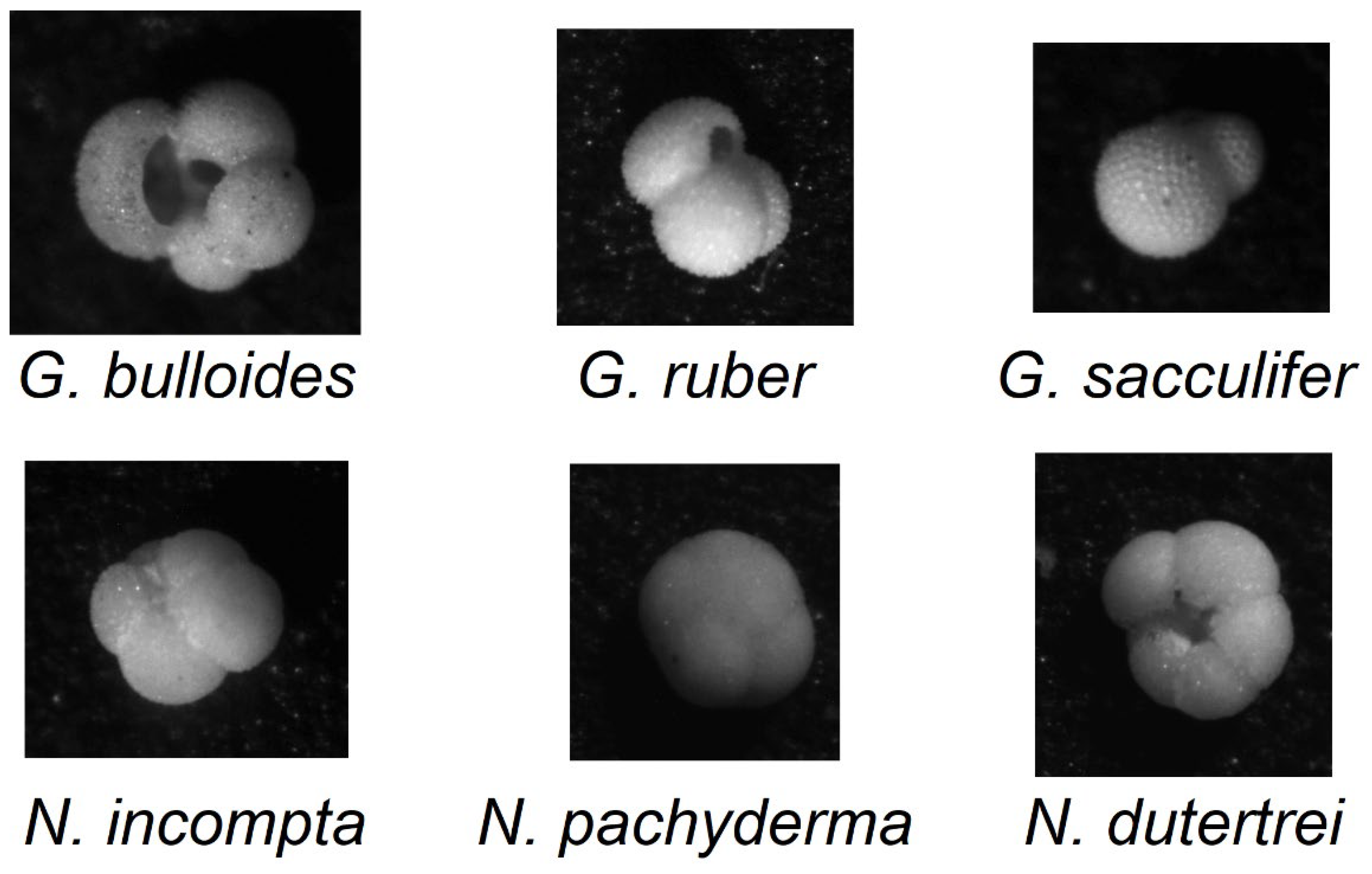
Figure 2.
Visual comparison of some RGB images of the EuroSAT dataset.
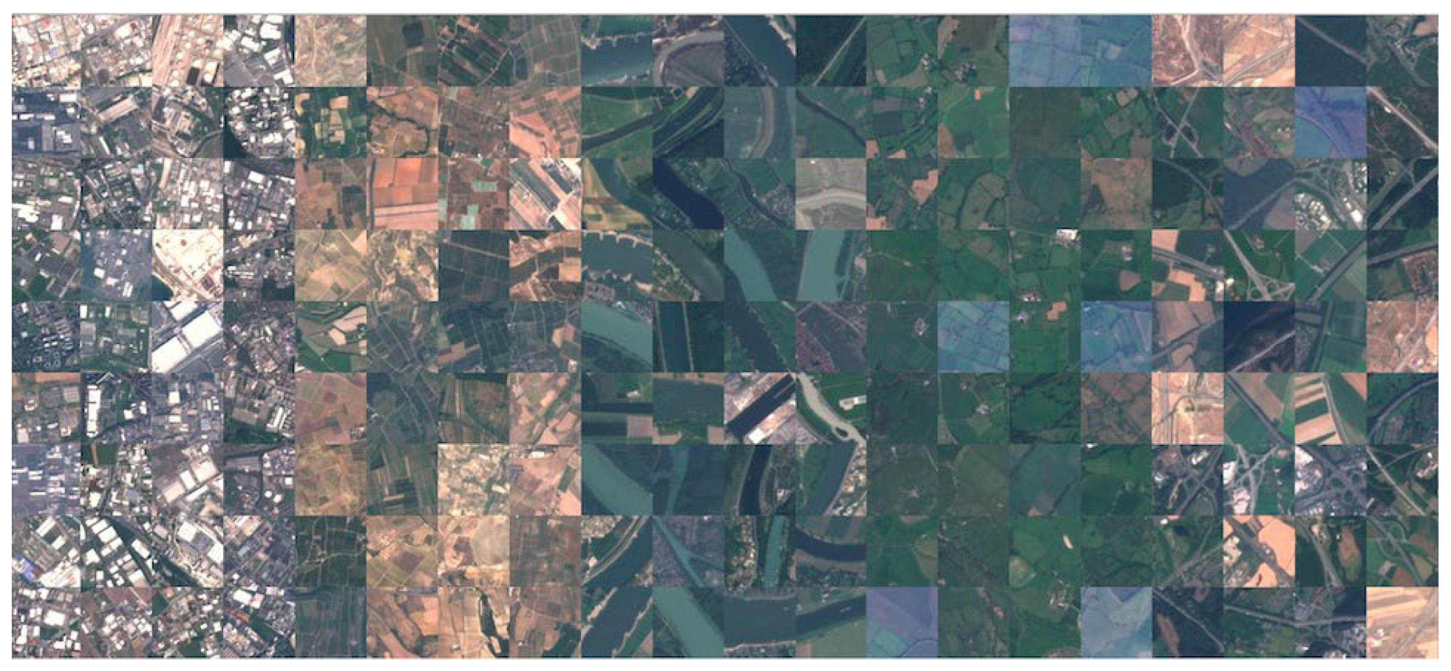

Table 1.
All thirteen bands captured by Sentinel-2’s Multispectral Imager (MSI) are detailed, including their identification, spatial resolution, and central wavelength for each spectral band.
Table 1.
All thirteen bands captured by Sentinel-2’s Multispectral Imager (MSI) are detailed, including their identification, spatial resolution, and central wavelength for each spectral band.
| Band | Spatial Central Resolution - meters | Wavelength - nanometre |
|---|---|---|
| B01 - Aerosols | 60 | 443 |
| B02 - Blue | 10 | 490 |
| B03 - Green | 10 | 560 |
| B04 - Red | 10 | 665 |
| B05 - Red edge 1 | 20 | 705 |
| B06 - Red edge 2 | 20 | 740 |
| B07 - Red edge 3 | 20 | 783 |
| B08 - NIR | 10 | 842 |
| B08A - Red edge 4 | 20 | 865 |
| B09 - Water vapor | 60 | 945 |
| B10 - Cirrus | 60 | 1375 |
| B11 - SWIR 1 | 20 | 1610 |
| B12 - SWIR 2 | 20 | 2190 |
Table 2.
Results obtained with each methodology on the Foraminifera dataset.
| Approach | F1-measure |
|---|---|
| [6] | 85.0 |
| [11] | 90.6 |
| GraySet(10)_Res | 89.4 |
| Random(10)_Res | 91.1 |
| Random(20)_Res | 91.3 |
| Random(20)_DN | 91.5 |
| Random(20)_MV2 | 90.2 |
| Res+DN | 91.8 |
| Res+DN+MV2 | 92.1 |
| DN+MV2 | 92.3 |
Table 3.
Precision, recall, accuracy and score comparison between the previous SOTA and the best ensemble presented here.
Table 3.
Precision, recall, accuracy and score comparison between the previous SOTA and the best ensemble presented here.
| Precision (%) | Recall (%) | F1 Score (%) | Accuracy (%) | |
| Human Novices (max) [6] | 65 | 64 | 63 | 63 |
| Human Experts (max) [6] | 83 | 83 | 83 | 83 |
| ResNet50 + Vgg16 [6] | 84 | 86 | 85 | 85 |
| Stand alone Vgg16 [6] | 80 | 82 | 81 | 81 |
| [11] | 90.9 | 90.6 | 90.6 | 90.7 |
| Res+DN | 91.1 | 92.8 | 91.8 | 91.7 |
| Res+DN+MV2 | 91.5 | 93.0 | 92.1 | 91.8 |
| DN+MV2 | 91.6 | 93.4 | 92.3 | 92.0 |
Table 4.
Accuracy obtained by each methodology on the EuroSAT dataset.
| Approach | Accuracy |
|---|---|
| RGB(1)_Res | 98.54 |
| RGB(5)_Res | 98.80 |
| Random(5)_Res | 98.57 |
| RandomOneRGB(5)_Res | 98.91 |
| RandomOneRGB(20)_Res | 98.94 |
| RandomOneRGB(20)_DN | 99.15 |
| Res+DN | 99.17 |
| Res+DN+MV2 | 99.22 |
| DN+MV2 | 99.20 |
| [36] | 99.24 |
| [37] | 99.22 |
| [38] | 99.20 |
| [39] | 98.96 |
Disclaimer/Publisher’s Note: The statements, opinions and data contained in all publications are solely those of the individual author(s) and contributor(s) and not of MDPI and/or the editor(s). MDPI and/or the editor(s) disclaim responsibility for any injury to people or property resulting from any ideas, methods, instructions or products referred to in the content. |
© 2024 by the authors. Licensee MDPI, Basel, Switzerland. This article is an open access article distributed under the terms and conditions of the Creative Commons Attribution (CC BY) license (http://creativecommons.org/licenses/by/4.0/).
Copyright: This open access article is published under a Creative Commons CC BY 4.0 license, which permit the free download, distribution, and reuse, provided that the author and preprint are cited in any reuse.


