Submitted:
20 December 2024
Posted:
23 December 2024
You are already at the latest version
Abstract
Multiple Input Multiple Output (MIMO) radar enjoys the advantages of high degree of freedom and relatively large virtual aperture, so it has various forms of applications in several aspects such as remote sensing, autonomous driving and radar imaging. Among all multiplexing schemes, Time-Division Multiplexing (TDM) MIMO radar gains a wide range of interests, as it has a simple and low-cost hardware system which is easy to implement. However, the time-division nature of TDM-MIMO leads to the dilemma between lower Pulse Repetition Interval (PRI) and more transmitters, as the PRI of a TDM-MIMO system is proportional to the number of transmitters while the number of transmitters significantly affects the resolution of MIMO radar. Moreover, a high PRI is often needed to obtain unambiguous imaging results for MIMO-SAR 3D imaging applications on a fast-moving platform such as a car or an aircraft. Therefore, it is of vital importance to develop an algorithm which can achieve unambiguous TDM-MIMO-SAR 3D imaging even when the PRI is low. Inspired by the motion compensation problem associated with TDM-MIMO radar imaging, this paper proposes a novel imaging algorithm which can utilize the phase shift induced by the time-division nature of TDM-MIMO radar to achieve unambiguous MIMO-SAR 3D imaging. A 2D-Compressed Sensing (CS) based method is employed and the proposed method is verified by simulation data. Finally, a real-world experiment is conducted to show the unambiguous imaging ability of the proposed method compared with the ordinary matched-filter-based method. The effect of velocity error is also analyzed with simulation results.
Keywords:
multiple input multiple output
; MIMO-SAR imaging
; compressed sensing
; unambiguous direction of arrival estimation
1. Introduction
In recent years, the Multiple Input Multiple Output (MIMO) technique, which achieves high Degree of Freedom (DOF) for radar systems, has drawn an increasing amount of attention in various applications, such as Autonomous Driving [1], Ground Penetrating Radar [2], Remote Sensing [3], Through-wall Imaging [4], etc. Orthogonal waveforms are radiated by transmitters (TXs), thus a MIMO system can separate different signals transmitted by different TXs. For example, a MIMO radar which has transmitters and receivers can generate virtual antennas. There are three multiplexing schemes to obtain waveform diversity, namely Time-Division Multiplexing (TDM), Frequency-Division Multiplexing (FDM) and Code-Division Multiplexing (CDM). Due to the advantages of low hardware complexity and high signal separation, TDM-MIMO system is easy to implement, thus it has a wide range of applications [5]. A large amount of research has focused on the algorithms and implementations for TDM-MIMO radar [6,7,8]. However, a TDM-MIMO system has an inherent drawback which limits its performance. As transmitters take turns to transmit their signal, phase errors occur in nonstationary scenarios [9]. In addition, more transmitters mean lower Pulse Repetition Frequency (PRF) and reduced maximum velocity that can be detected [5].
Synthetic Aperture Radar (SAR) is an important technique for remote sensing and radar imaging. With the help of MIMO technology, a new architecture called MIMO-SAR not only increases spatial resolution [10], but also provides novel imaging capability such as 3D imaging [11] and Ground-Moving Target Indication (GMTI) [12]. Due to the great potential of MIMO-SAR architecture, many researchers have contributed to various aspects of MIMO-SAR. In [10], it is shown that the mere use of orthogonal waveforms is insufficient for most SAR applications, and thus a new class of waveform is introduced. Yanik et al. addressed the issues of the design process of MIMO-SAR systems and presents three versions of MIMO-SAR testbeds with different costs and performances [13]. As in many cases, such as Unmanned Aerial Vehicle (UAV) imaging, irregular scanning geometries and computational complexity limit the capability of MIMO-SAR systems, Smith et al. proposed a new algorithm to leverage SAR and MIMO while achieving high resolution with high efficiency near field MIMO-SAR imaging [14]. The effect of virtual array approximation in near field applications is studied by Hu et al., and a new design criterion is presented [15]. An efficient image reconstruction algorithm which avoids time-consuming wavenumber accumulation by decomposing the range-wavenumber based on binomial approximation theory is proposed for MIMO-SAR 3D imaging [16]. A beat frequency division (BFD) frequency-modulated continuous wave (FMCW) MIMO-SAR system and the corresponding signal process method which are suitable for UAV environments are presented [17]. With appropriate transformation, MIMO-SAR 3D imaging can be achieved by inverse Fourier transform (IFT) [18].
Apart from the imaging algorithms and array design of MIMO-SAR, it is the realization of MIMO systems that significantly affect both the performance and costs of MIMO-SAR. There are numerous studies discussing the problem of MIMO-SAR associated with a specific MIMO realization. Jin et al. proposed a novel MIMO-SAR scheme based on segmented-phase-code waveform which can relieve the short-term shift-orthogonality condition without losing imaging performance [19]. In [20], a MIMO-SAR system using chirp diverse waveform is discussed to achieve high resolution for wide-swath remote sensing, as chirp diverse waveform can easily provide high bandwidth which is necessary for this radar imaging. It is acknowledged that a large time-bandwidth product, low cross-correlation interferences and a low peak-average ratio have significant importance for MIMO radar imaging. To reach these aims, an orthogonal frequency division multiplexing (OFDM) chirp waveform with random matrix modulation is proposed for MIMO-SAR applications [21]. As mentioned before, TDM-MIMO enjoys many advantages with respect to hardware complexity and cost. A forward-looking MIMO-SAR enhanced imaging scheme is presented, and its performance is validated with a TDM-MIMO radar [22]. In [23], the authors proposed a hierarchical high-resolution MIMO-SAR imaging algorithm which is derived in case of TDM-MIMO realization and the algorithm is tested on a TDM-MIMO system. There are also several researches focused on near-field imaging [24], Ground Based SAR(GB-SAR) applications [25]. To tackle the problem of ghost targets caused by sparse MIMO array, an algorithm called Sequential Spatial Masking (SSM) is proposed for forward-looking TDM-MIMO-SAR imaging [26]. As discussed above, the nature of TDM-MIMO brings challenges to imaging algorithms in nonstationary scenarios because different transmitters are activated separately. Since Synthetic Aperture Radar (SAR) systems rely on the relative movement between platforms and targets, TDM-MIMO brings difficulties to using TDM-MIMO for SAR imaging [27]. Besides, to achieve higher resolution with TDM-MIMO array, it is often required to have more transmitters, which leads to a lower PRF. However, if a MIMO-SAR system is installed on a fast-moving platform, such as a car or an aircraft, a low PRF means grating lobes and ghost targets appears in SAR imaging process. Notably, it is the time-division nature of TDM-MIMO that brings obstacles to its applications MIMO-SAR 3D imaging on a fast-moving platform.
To further improve imaging capabilities of MIMO-SAR technique, the super-resolution algorithms are also applied and modified for MIMO-SAR imaging. Traditional imaging methods, which lack the super-resolution ability, are well-researched in MIMO imaging scenarios. For instance, back projection (BP) [28] and rang migration (RM) [29] have been implemented in high-resolution MIMO imaging. However, the performances of these methods highly depend on the aperture of virtual array. To further improve imaging ability, the compressed sensing theory, which has been strictly proved [30], are widely used in radar imaging, including MIMO imaging and ISAR imaging [31]. Therefore, numerous research has been focused on modifying and improving CS-based methods for MIMO and MIMO-SAR 3D imaging. In [32], the author proposed a CS-based method combined with a 2-step motion compensation process for MIMO-SAR imaging. In [33], a L1-norm minimization method is used to do spatial filtering for deep neural network (DNN) for MIMO-SAR 3D imaging in low signal-to-noise ratio (SNR) scenarios. Z. Zhou et al. [34] made a comparison of BP and sparse Bayesian recovery via iterative minimum (SBRIM) and concluded that generally SBRIM has better imaging ability but suffers from high computational complexity. A tensor compressed sensing algorithm is proposed for 3D imaging with Cross-MIMO array [35]. An efficient MIMO-SAR imaging algorithm based on alternating direction method of multipliers (ADMM) is conducted and validated by experimental results [36]. Most existing researches focus on computational efficiency, motion compensation and multipath effect. However, few researchers pay attention to super-resolution MIMO-SAR 3D imaging while considering the unique nature of TDM-MIMO.
This article is mainly contributed to utilizing the property of TDM-MIMO to achieve unambiguous MIMO-SAR 3D imaging on a fast-moving platform. As discussed in paragraphs above, if a TDM-MIMO radar employs more transmitters to achieve high resolution, it will also have a lower PRF which makes MIMO-SAR imaging ambiguous on a fast-moving platform, such as a car or an aircraft. In this article, a novel CS-based super-resolution algorithm is proposed to achieve unambiguous MIMO-SAR 3D imaging by making good use of the phase shift caused by motion of platform. Through both simulation and real data experiments, we show that our algorithm perform well on a fast moving platform, while other methods fail.
2. Signal Model
In this section, the signal model of TDM-MIMO-SAR 3D imaging is deduced and simplified. Moreover, our deductions are verified by simulation data.
The geometry of TDM-MIMO-SAR 3D imaging is shown in Figure 1. Figure 1(a) demonstrates the imaging scenario of a typical airborne sensing application with a linear MIMO array of 4 transmitters and 8 receivers. For simplicity, an equivalent geometry is demonstrated in Figure 1(b) where only one single point target is shown with its coordinates. In the following discussion, we will follow the notation and geometry depicted in Figure 1(b), where the x axis, y axis and z axis stand for the cross-track direction, the track direction and the height direction. The linear TDM-MIMO array is distributed along the z axis, and thus the height resolution is provided by the MIMO array. The platform is moving along the y axis with a velocity . The MIMO array composed of transmitters and receivers can be equivalent to virtual elements. The inter-element space of transmitters and receivers are and . stands for the wavelength of the transmitted signal. For a typical time-division working mode, it can be assumed that all receivers are activated during the entire TDM period, while transmitters take turns to transmit radar waves. A single TDM period contains pulses and each pulse lasts for seconds. So, a full TDM period lasts for seconds. To complete a MIMO-SAR imaging working circle, it takes TDM periods to transmit pulses.
It is well known that virtual array approximation is useful and sufficient for most MIMO applications. In a TDM-MIMO-SAR working mode shown in Figure 1(b), the equivalent virtual array is distributed in a two-dimensional aperture shown in Figure 2. As discussed before, each TDM period costs for seconds and the entire working circle which contains TDM period lasts for seconds. With a platform velocity of m/s along y axis, the aperture length along y axis is m, while the aperture length along z axis is m. However, it is shown in Figure 2 that due to the property of time-division working mode, virtual elements of the same TDM period are not exactly distributed on the same line. For instance, if we assume the coordinates of the first sub-aperture of virtual elements in the first TDM period are , the coordinates of the second sub-aperture in the first TDM period are . There are several motion compensation methods developed to achieve 3D imaging for TDM-MIMO radar. However, these methods cannot exploit the full potential of TDM-MIMO-SAR. In the following sections, we will demonstrate a novel algorithm which can exploit this property of TDM-MIMO to achieve unambiguous 3D imaging.
For simplicity, we assume that the coordinates of the platform at time are , thus the transmitters are at and the receivers are at . With a velocity towards y axis, the platform moves to at the TDM period. Suppose that there are targets with corresponding coordinates . For a virtual element synthesized by the transmitter and the receiver, the baseband receiver signal reflected by the target is written as
Where denotes the fast time of one pulse, is the reflection coefficient of the targets and is the baseband signal transmitted by antennas. For simplicity, we assume that a chirp signal which is widely used in radar imaging is employed in the MIMO-SAR application.
Where represents the slope of the frequency change and is the carrier frequency. For a de-chirping process, the received signal is multiplied by the complex conjugate of the transmitted signal.
A Fast Fourier Transform (FFT) can be conducted to complete the de-chirping process.
Where represents the range bin. The equation above can be further simplified and rewritten as
means that the target is on the range bin. Sum up reflected signals of all targets and gaussian noise. After the de-chirping process, the four-dimensional sampled data can be expressed as
Where represents an additive white gaussian noise. According to the virtual array approximation, equation (7) can be approximated to a more concise form. The coordinates of virtual element of the transmitter and receiver discussed above, which is the virtual element, should be . For simplicity, this virtual element is called the virtual element and the distance between the virtual element and the target is denoted as .
Similarly, can also be approximated according to the virtual element approximation.
By combining the equation (12) and equation (13), we get an approximation of equation (7). The second approximation in equation (14) is done by the far field assumption.
With the virtual array approximation, the four-dimensional data can be reshaped to a three-dimensional cube shown in Figure 3. For simplicity, we assume that is small enough that range cell migration does not happen in one MIMO-SAR working circle and both the synthetic aperture and MIMO aperture are significantly smaller than the rang distance of the target and the radar, such that the far field assumption can be established.
By dividing the data into separate 2d matrix, we can further simplify the 3D imaging problem to a 2D imaging problem in every range bins. Suppose that the target is in the range bin. The corresponding 2d data matrix can be denoted as
Where represents the virtual element and represents the TDM-period. The coordinates of this virtual element are . By introducing the far-field assumption, the equation (15) can be simplified.
Equation (17) is a result of ignoring constant term and quadratic term while substituting (16) for (15). The echo signal can be expressed as:
It is shown clearly in equation (18) that the TDM-MIMO-SAR 3D imaging is different from a naïve 2d imaging problem, as the property of time-division working mode introduces additional phase shift. Moreover, the phase shift is proportional to the exact of the target location. By simulation, our deduction can be validated in Figure 4. Figure 4 shows a simulation of a TDM-MIMO-SAR echo signal data after pulse compression. Details about the simulation settings are listed in Table 1.
3. Algorithm
In this section, we will firstly demonstrate a matched filter-based method with phase compensation for TDM-MIMO-SAR 3D imaging. Although this matched filter-based method performs well when the platform velocity is low, simulations show its limits when the platform moves fast due to gating lobes. Then we will show our proposed CS-based super-resolution method and its ability to suppress gating lobes for a TDM-MIMO-SAR on a fast-moving platform. To reduce the computational complexity, a 2D CS method is employed to reduce the computational complexity after regrouping the echo signal data.
3.1. The Matched Filter-based Imaging Scheme
To make a comparison, a conventional matched-filter based imaging scheme is demonstrated in this section. Following the deduction shown in Section 2, a straightforward matched filter-based imaging scheme with phase compensation is shown in Figure 5.
According to equation (18), the phase compensation term is expressed as
The MF-based algorithm provides imaging results without super-resolution capability. Moreover, it does not utilize the phase shift caused by the TDM working mode to deal with gating lobes which occur when the platform moves fast. A simulation result shown in Figure 6 will demonstrate how gating lobes affect the imaging process of MIMO-SAR as the velocity of the platform increases. The detailed parameters of this simulation are the same as parameters listed in Table 1. The number of TDM-periods is 16. The geometry of imaging process is shown in Figure 2.
For real world MIMO-SAR applications, a fast-moving platform, such as a car or an aircraft, is a common situation. Although it is possible to avoid the gating lobes problem by reducing PRI. However, the PRI of TDM-MIMO mainly depends on the number of transmitters and reducing the number of transmitters significantly affects the number of virtual elements, which is vital for MIMO radar ability. For TDM-MIMO enjoys the advantage of low hardware complexity and costs, it is important to develop a new algorithm for TDM-MIMO-SAR applications which can deal with the gating lobes problem so that combining the powerful capability of MIMO-SAR imaging scheme and the low complexity advantage of TDM-MIMO can be feasible on fast-moving platforms.
3.2. Proposed 2D-CS based Imaging Scheme
In this section, we demonstrate our proposed imaging algorithm based on regrouping echo data and 2D-CS super-resolution method. A brief mathematical proof is provided, and numerical simulation is conducted to compare the proposed method and other methods.
3.1.1. Compressed Sensing Theory and Methods
Let denotes a signal of finite length . There exists a basis matrix such that , where is a K-sparse vector with length . For a K-sparse vector, can be approximated by its largest coefficients. Let denotes the measurement matrix. The measured signal can be expressed as
Recovering from is an ill-posed problem for . However, according to the CS theory, the recovery is possible as long as has the Restricted Isometry Property (RIP). The detailed expression of RIP property is given as follows:
Although it is difficult to validate whether a not a measurement matrix satisfies the RIP directly, RIP is usually satisfied if the rows of and columns of are incoherent. With the help of RIP, the recovery problem is equal to solving the optimization problem which can be expressed as
However, the discontinuousness of norm leads to the difficulty of solving optimization problem (21). Therefore, there are many CS methods solving the optimization problem by applying relaxation of norm. For instance, the smoothed (SL0) method and method. In this article, we mainly focus on the method which can be denoted as
Moreover, the constrained optimization problem (22) can be converted to the unconstrained convex optimization problem shown in (23).
Where . An efficient approach to solve the problem (23) is the fast iterative shrinkage-thresholding algorithm (FISTA). By applying proximal gradient and Nesterov’s acceleration, the FISTA enjoys the advantage of both efficiency and accuracy. The detailed procedure of the FISTA is listed in Table 3.
By applying the two-dimensional model of norm optimization problem, a 2D-CS model can be expressed as
Where , , , . Therefore, after applying the proximal gradient with the optimization problem (24), we can get
Where and . It is obvious that is convex and follows the Lipschitz continuity.
Then the approximation of can be expressed as
The proximal gradient of is the gradient of .
The optimal solution of the proximal gradient can be achieved when the equation (28) is equal to . Therefore, the optimal solution is
Now, we substitute (25) into (29).
With the help of Nesterov’s acceleration, the detailed procedure of 2D-FISTA is demonstrated in Table 4.
3.1.2. The Proposed Algorithm
Following the expression in the equation (18), a novel algorithm which can utilize the property of TDM-MIMO to achieve unambiguous MIMO-SAR 3D imaging. In this section, first we analyze the motion-induced phase shift along the virtual array, then the full procedure of the proposed algorithm is demonstrated. Finally, the performance of the proposed algorithm is verified by simulation data.
After slow time compressing of the 2d data shown the equation (18) by MF methods or super-resolution methods, the 2d data is denoted as
For a point target , the corresponding signal after ignoring constant term is
With proper phase compensation shown in (19), the compensated 2d data is
However, as discussed previously, for a TDM-MIMO radar, it needs more transmitters to obtain more degree of freedom for MIMO imaging, while the increasing number of transmitters directly leads to the decreasing of PRF. And for MIMO-SAR applications, low PRF usually leads to ambiguous imaging results. Assume that for the point target , it has a gating lobe located at . After the phase compensation in (33), the corresponding signal is
Where .The main idea of our proposed method is to distinguish the real target and its gating lobe, so that an unambiguous MIMO-SAR 3D image can be achieved. Now, we apply the 2D-FISTA demonstrated in Table 4 to the phase-compensated 2D signal .
Where , , , , , , . Measurement matrix and consists of steering vectors and , , . is the number of atoms in the dictionary, which contains .
After 2D-FISTA process, a 2D result is obtained.
For a real target and its corresponding signal , its imaging result appear on the main diagonal of . On the other hand, for a gating lobe, its imaging result is located off the main diagonal, as it is shown in the equation (38). Based on the equation (33) and (34), we can obtain
By extracting the main diagonal of , we manage to achieve unambiguous MIMO-SAR 3D imaging. A simulation result shown in Figure 7 demonstrates how the real target differs from gating lobes in the 2D result obtained by equation (35). The simulation settings are the same as in Figure 6.
As is clearly shown in Figure 7, the proposed scheme manages to eliminate gating lobes which distribute along y axis. After the phase compensation and 2D-CS process, the gating lobes should be filtered by extracting the main diagonal. Therefore, although the imaging result along y axis is ambiguous, the gating lobes would not appear in the final 3D imaging result as gating lobes are filtered and eliminated.
The full imaging scheme is demonstrated in Figure 8.
3.3. Simulation Results
In this section, the imaging effects of the proposed method in the TDM-MIMO-SAR 3D imaging are analyzed by simulation results. A comparison of the ordinary MF-based method and the proposed method is made to demonstrate the difference between ambiguous imaging results and unambiguous ones. The major parameters of this simulation test are listed in Table 6. The geometry of the MIMO-SAR imaging is shown in Figure 2.
As can be seen from simulation results shown in Figure 9, the MF-based method suffers from gating lobes when the platform velocity is high. The increasing of the platform velocity severely degrades the imaging result of the MF-based method, meanwhile the proposed method manages to achieve unambiguous imaging.
As is demonstrated in Table 5, the process of the proposed method relies on information about the velocity of the platform. In real world applications, the measured velocity may not be the exact velocity. Therefore, it is vital to analyze the effect of velocity error. In this section, the effect of velocity error is analyzed by simulation results under the same setup as shown in Table 6. The simulation of the proposed method under velocity error is demonstrated in Figure 10.
It is indicated in simulation results that although the velocity error indeed degrades the imaging performance of the proposed method, the proposed method still maintains unambiguous imaging capability with a velocity error less than 10% of the exact velocity.
4. Experimental and Analysis
In this section, a real world TDM-MIMO-SAR 3D imaging experiment is conducted to verify the proposed method. An AWR2243 cascaded MIMO radar is used to collect measured data. Developed by Texas Instruments (TI), AWR2243 is a multichannel array radar with short-range MIMO imaging capability. The key parameters of AWR2243 in MIMO mode are shown in Table 7.
Among all 12 transmitters of AWR2243, 9 of these transmitters are placed in a uniform linear array. Detailed structure of AWR2243 is shown in Figure 11.
As shown in Figure 12(a)(b), the MIMO radar system is installed on a moving vehicle which can reach 3 m/s. The platform moves along a straight road as indicated in Figure 12(c). Three corner reflectors are set by the road as shown in Figure 12(d). It is clearly shown in Figure 12(e) that gating lobes occur in the experiment circumstance. Figure 12(f) demonstrates the proposed method’s ability for unambiguous MIMO-SAR imaging.
To further demonstrate the performance of the proposed method under more realistic circumstances, we installed the AWR2243 radar on an actual car which runs at a speed of 20km/h as shown in Figure 13. The main target is a stationary car by the road which the platform is moving along. Figure 13(c, d) demonstrates the 2D projection of the MF-based method and the proposed method and it is clearly shown that the proposed method effectively eliminates the gating lobes and achieves unambiguous MIMO-SAR imaging.
5. Conclusions
In this paper, an unambiguous MIMO-SAR 3D imaging algorithm is proposed for applications on a fast-moving platform with TDM-MIMO. For TDM-MIMO radar, an increase of the number of transmitters significantly decreases the PRF of each transmitter, which leads to ambiguous MIMO-SAR imaging for a fast-moving platform, making it necessary to develop an unambiguous TDM-MIMO-SAR imaging algorithm. By analyzing the detailed virtual array geometry and the corresponding signal model of TDM-MIMO-SAR, we manage to utilize the phase shift induced by the time division property to solve the ambiguity of MIMO-SAR imaging. A 2D-CS method based on FISTA is used in the proposed methods for super-resolution imaging. Compared with the MF-based method, the proposed method successfully eliminates gating lobes and thus achieve unambiguous MIMO-SAR imaging. The performance of the proposed method is verified by both simulation data and real-world experiments. In order to fulfill the requirements of real world applications, the effect of velocity error is analyzed by simulation results. The main contribution of this paper is to propose a super-resolution method which can utilize the time-division property of TDM-MIMO radar to solve ambiguity of MIMO-SAR imaging.
Supplementary Materials
The following supporting information can be downloaded at: www.mdpi.com/xxx/s1, Figure S1: title; Table S1: title; Video S1: title.
Author Contributions
Conceptualization, S. Guan, Y. Li, X. Liang, M. Wang; methodology, S. Guan, Y. Li and Y. Liu.; software, S. Guan and Y. Liu; investigation, S. Guan; resources, Y. Li and X. Liang; writing, S. Guan and Y. Li; project administration, M. Wang and Y. Li. All authors have read and agreed to the published version of the manuscript.
Funding
Please add: “This research received no external funding” or “This research was funded by NAME OF FUNDER, grant number XXX” and “The APC was funded by XXX”. Check carefully that the details given are accurate and use the standard spelling of funding agency names at https://search.crossref.org/funding. Any errors may affect your future funding.
Data Availability Statement
We encourage all authors of articles published in MDPI journals to share their research data. In this section, please provide details regarding where data supporting reported results can be found, including links to publicly archived datasets analyzed or generated during the study. Where no new data were created, or where data is unavailable due to privacy or ethical restrictions, a statement is still required. Suggested Data Availability Statements are available in section “MDPI Research Data Policies” at https://www.mdpi.com/ethics.
Acknowledgments
We particularly appreciate students of Aerospace Information Research Institute, Chinese Academy of sciences who contributed to help with experiments. These students are Miaomiao Li, Jiasheng Cao and Zhiyuan Zeng. Besides, Dr. Denggao Guan who is an associate professor of Chengdu University of Technology, together with his wife Yanzhen Qu, also helped with our experiments.
Conflicts of Interest
The authors declare no conflicts of interest.
References
- Sun, S.; Petropulu, A.P.; Poor, H.V. MIMO radar for advanced driver-assistance systems and autonomous driving: Advantages and challenges. IEEE Signal Processing Magazine 2020, 37, 98-117.Jin, T., et al. (2012). "Extraction of Landmine Features Using a Forward-Looking Ground-Penetrating Radar With MIMO Array." IEEE Transactions on Geoscience and Remote Sensing 50(10): 4135-4144.
- Tarchi, D.; Oliveri, F.; Sammartino, P.F. MIMO radar and ground-based SAR imaging systems: Equivalent approaches for remote sensing. IEEE Transactions on Geoscience and Remote Sensing 2012, 51, 425–435. [Google Scholar] [CrossRef]
- Ralston, T.S.; Charvat, G.L.; Peabody, J.E. Real-time through-wall imaging using an ultrawideband multiple-input multiple-output (MIMO) phased array radar system. In Proceedings of the 2010 IEEE international symposium on phased array systems and technology; 2010; pp. 551–558. [Google Scholar]
- Li, X.; Wang, X.; Yang, Q.; Fu, S. Signal processing for TDM MIMO FMCW millimeter-wave radar sensors. IEEE Access 2021, 9, 167959–167971. [Google Scholar] [CrossRef]
- Rambach, K.; Yang, B. MIMO radar: Time division multiplexing vs. code division multiplexing. 2017. [Google Scholar]
- Taparugssanagorn, A.; Ylitalo, J.; Fleury, B.H. Phase-noise in TDM-switched MIMO channel sounding and its impact on channel capacity estimation. In Proceedings of the IEEE GLOBECOM 2007-IEEE Global Telecommunications Conference; 2007; pp. 4559–4564. [Google Scholar]
- Luo, J.; Zhang, Y.; Yang, J.; Zhang, D.; Zhang, Y.; Zhang, Y.; Huang, Y.; Jakobsson, A. Online sparse DOA estimation based on sub–aperture recursive LASSO for TDM–MIMO radar. Remote Sensing 2022, 14, 2133. [Google Scholar] [CrossRef]
- Bechter, J.; Roos, F.; Waldschmidt, C. Compensation of motion-induced phase errors in TDM MIMO radars. IEEE Microwave and Wireless Components Letters 2017, 27, 1164–1166. [Google Scholar] [CrossRef]
- Krieger, G. MIMO-SAR: Opportunities and pitfalls. IEEE transactions on geoscience and remote sensing 2013, 52, 2628–2645. [Google Scholar] [CrossRef]
- Zhuge, X.; Yarovoy, A.G. A sparse aperture MIMO-SAR-based UWB imaging system for concealed weapon detection. IEEE Transactions on Geoscience and Remote Sensing 2010, 49, 509–518. [Google Scholar] [CrossRef]
- Wang, W.-Q.; Cai, J. Ground moving target indication by MIMO SAR with multi-antenna in azimuth. In Proceedings of the 2011 IEEE International Geoscience and Remote Sensing Symposium; 2011; pp. 1662–1665. [Google Scholar]
- Yanik, M.E.; Wang, D.; Torlak, M. Development and demonstration of MIMO-SAR mmWave imaging testbeds. IEEE Access 2020, 8, 126019–126038. [Google Scholar] [CrossRef]
- Smith, J.W.; Torlak, M. Efficient 3-D near-field MIMO-SAR imaging for irregular scanning geometries. IEEE Access 2022, 10, 10283–10294. [Google Scholar] [CrossRef]
- Hu, C.; Wang, J.; Tian, W.; Zeng, T.; Wang, R. Design and imaging of ground-based multiple-input multiple-output synthetic aperture radar (MIMO SAR) with non-collinear arrays. Sensors 2017, 17, 598. [Google Scholar] [CrossRef]
- Yang, G.; Li, C.; Wu, S.; Liu, X.; Fang, G. MIMO-SAR 3-D imaging based on range wavenumber decomposing. IEEE Sensors Journal 2021, 21, 24309–24317. [Google Scholar] [CrossRef]
- Kim, S.; Yu, J.; Jeon, S.-Y.; Dewantari, A.; Ka, M.-H. Signal processing for a multiple-input, multiple-output (MIMO) video synthetic aperture radar (SAR) with beat frequency division frequency-modulated continuous wave (FMCW). Remote Sensing 2017, 9, 491. [Google Scholar] [CrossRef]
- Lin, B.; Li, C.; Ji, Y.; Liu, X.; Fang, G. A Millimeter-Wave 3D Imaging Algorithm for MIMO Synthetic Aperture Radar. Sensors 2023, 23, 5979. [Google Scholar] [CrossRef]
- Jin, G.; Deng, Y.; Wang, W.; Wang, R.; Zhang, Y.; Long, Y. Segmented phase code waveforms: A novel radar waveform for spaceborne MIMO-SAR. IEEE Transactions on Geoscience and Remote Sensing 2020, 59, 5764–5779. [Google Scholar] [CrossRef]
- Wang, W.-Q.; Cai, J. MIMO SAR using chirp diverse waveform for wide-swath remote sensing. IEEE Transactions on Aerospace and Electronic Systems 2012, 48, 3171–3185. [Google Scholar] [CrossRef]
- Wang, W.-Q. MIMO SAR OFDM chirp waveform diversity design with random matrix modulation. IEEE Transactions on Geoscience and Remote Sensing 2014, 53, 1615–1625. [Google Scholar] [CrossRef]
- Albaba, A.; Bauduin, M.; Verbelen, T.; Sahli, H.; Bourdoux, A. Forward-looking MIMO-SAR for enhanced radar imaging in autonomous mobile robots. IEEE Access 2023. [Google Scholar] [CrossRef]
- Gao, X.; Roy, S.; Xing, G. MIMO-SAR: A hierarchical high-resolution imaging algorithm for mmWave FMCW radar in autonomous driving. IEEE Transactions on Vehicular Technology 2021, 70, 7322–7334. [Google Scholar] [CrossRef]
- Wu, C.; Liu, Y.; Zhu, L.; Li, R. Near-field SAR mmWave Image Reconstruction With Noise Reduction Using TDM-MIMO. In Proceedings of the 2022 International Conference on Frontiers of Communications, Information System and Data Science (CISDS); 2022; pp. 79–83. [Google Scholar]
- Zhang, Z.; Suo, Z.; Tian, F.; Qi, L.; Tao, H.; Li, Z. A Novel GB-SAR System Based on TD-MIMO for High-Precision Bridge Vibration Monitoring. Remote Sensing 2022, 14, 6383. [Google Scholar] [CrossRef]
- Albaba, A.; Bauduin, M.; Sakhnini, A.; Sahli, H.; Bourdoux, A. Sidelobes and Ghost Targets Mitigation Technique for High-Resolution Forward-Looking MIMO-SAR. IEEE Transactions on Radar Systems 2024, 2, 237–250. [Google Scholar] [CrossRef]
- Farhadi, M.; Feger, R.; Fink, J.; Wagner, T.; Stelzer, A. Automotive synthetic aperture radar imaging using tdm-mimo. In Proceedings of the 2021 IEEE Radar Conference (RadarConf21); 2021; pp. 1–6. [Google Scholar]
- Chen, A.-L.; Wang, D.-w.; Ma, X.-y. An improved BP algorithm for high-resolution MIMO imaging radar. In Proceedings of the 2010 International Conference on Audio, Language and Image Processing; 2010; pp. 1663–1667. [Google Scholar]
- Zhuge, X.; Yarovoy, A.G. Three-dimensional near-field MIMO array imaging using range migration techniques. IEEE Transactions on Image Processing 2012, 21, 3026–3033. [Google Scholar] [CrossRef]
- Donoho, D.L. Compressed sensing. IEEE Transactions on information theory 2006, 52, 1289–1306. [Google Scholar] [CrossRef]
- Zhang, L.; Xing, M.; Qiu, C.-W.; Li, J.; Bao, Z. Achieving higher resolution ISAR imaging with limited pulses via compressed sampling. IEEE Geoscience and Remote Sensing Letters 2009, 6, 567–571. [Google Scholar] [CrossRef]
- Gu, F.-F.; Zhang, Q.; Chi, L.; Chen, Y.-A.; Li, S. A novel motion compensating method for MIMO-SAR imaging based on compressed sensing. IEEE Sensors Journal 2014, 15, 2157–2165. [Google Scholar] [CrossRef]
- Wu, C.; Zhang, Z.; Chen, L.; Yu, W. Super-resolution for MIMO array SAR 3-D imaging based on compressive sensing and deep neural network. IEEE Journal of Selected Topics in Applied Earth Observations and Remote Sensing 2020, 13, 3109–3124. [Google Scholar] [CrossRef]
- Zhou, Z.; Wei, S.; Wang, M.; Liu, X.; Wei, J.; Shi, J.; Zhang, X. Comparison of MF and CS algorithm in 3-D near-field SAR imaging. In Proceedings of the 2021 7th Asia-Pacific Conference on Synthetic Aperture Radar (APSAR); 2021; pp. 1–5. [Google Scholar]
- Feng, W.; Friedt, J.-M.; Nico, G.; Sato, M. 3-D ground-based imaging radar based on C-band cross-MIMO array and tensor compressive sensing. IEEE Geoscience and Remote Sensing Letters 2019, 16, 1585–1589. [Google Scholar] [CrossRef]
- Chen, X.; Luo, C.; Yang, Q.; Yang, L.; Wang, H. Efficient MMW image reconstruction algorithm based on ADMM framework for near-field MIMO-SAR. IEEE Transactions on Microwave Theory and Techniques 2023. [Google Scholar] [CrossRef]
Figure 1.
The geometry of MIMO-SAR 3D imaging: (a) a typical example of an airborne MIMO-SAR application with a linear MIMO array; (b) a simplified situation of point targets imaging scenario.
Figure 1.
The geometry of MIMO-SAR 3D imaging: (a) a typical example of an airborne MIMO-SAR application with a linear MIMO array; (b) a simplified situation of point targets imaging scenario.
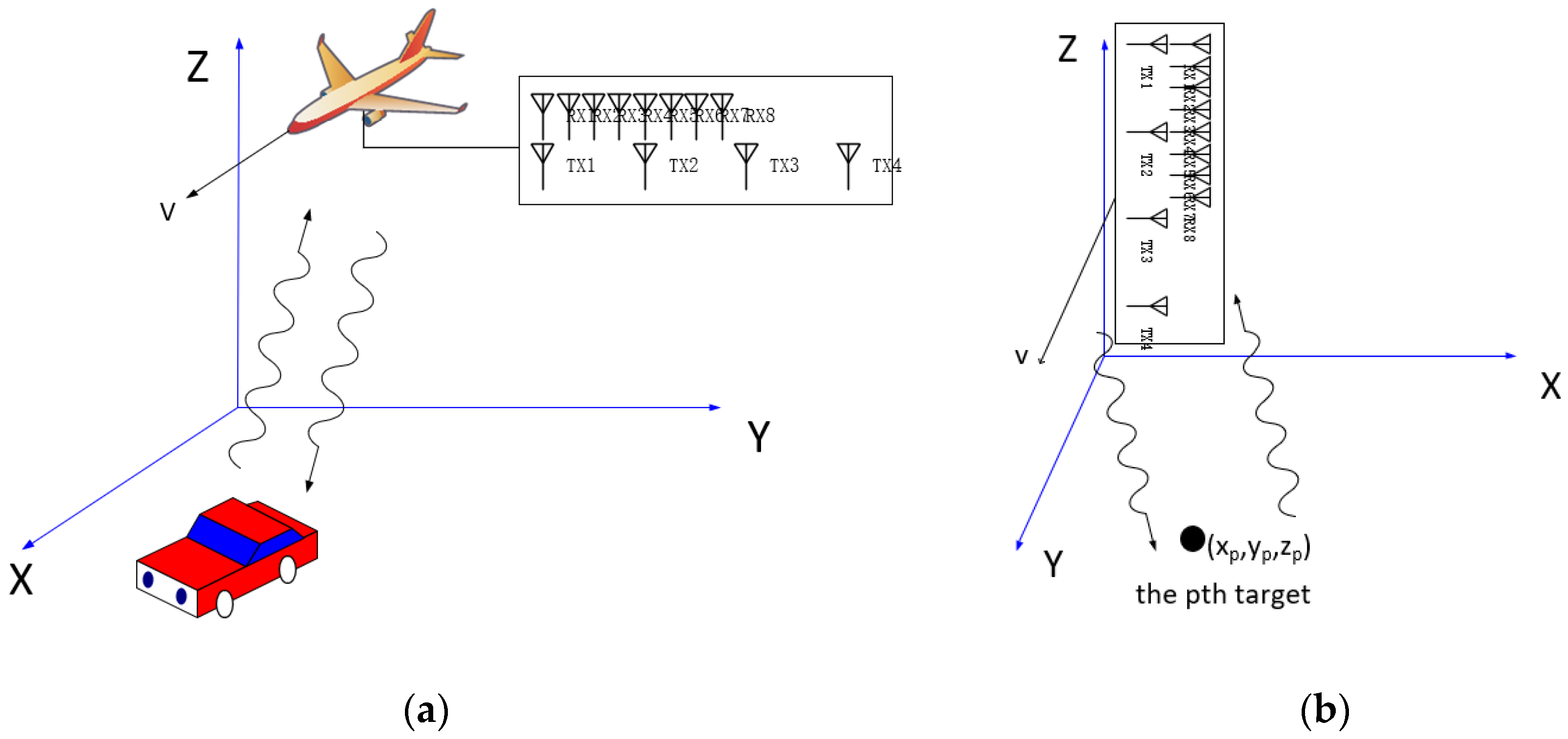
Figure 2.
The geometry of virtual array approximation for TDM-MIMO-SAR 3D imaging.
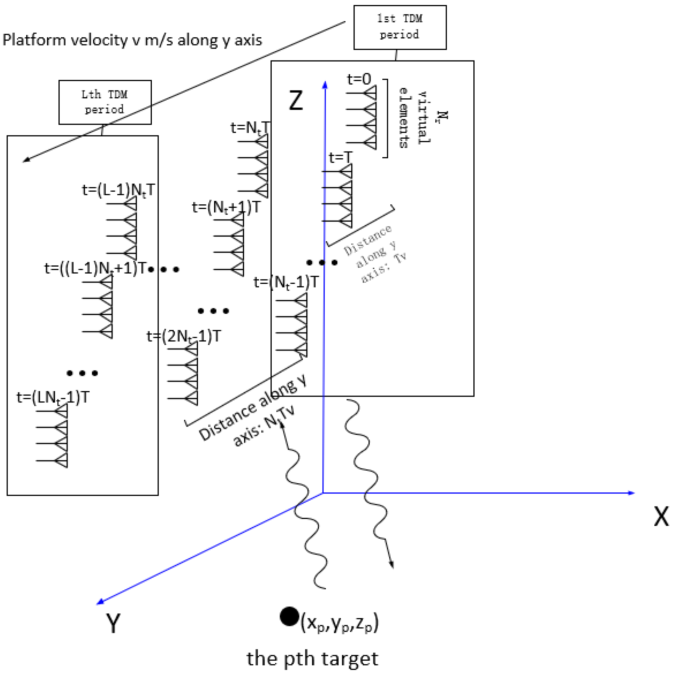
Figure 3.
The three-dimensional data cube after range compression.
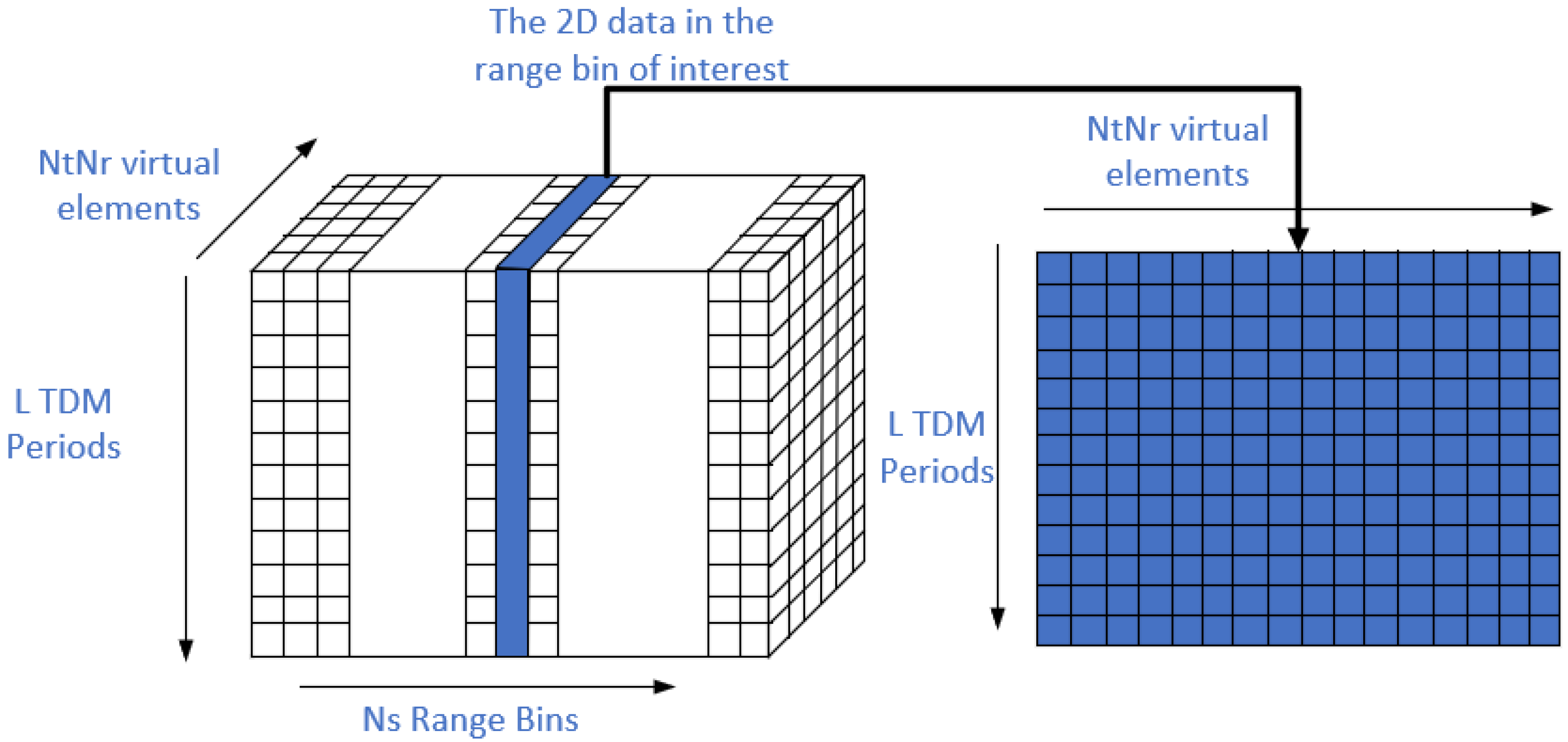
Figure 4.
The measured phase of the echo signal in the same range bin and the same TDM period of one point target after pulse compression: (a) the measured phase of 32 virtual elements, when and . (b) the measured phase of 32 virtual elements, when and .
Figure 4.
The measured phase of the echo signal in the same range bin and the same TDM period of one point target after pulse compression: (a) the measured phase of 32 virtual elements, when and . (b) the measured phase of 32 virtual elements, when and .
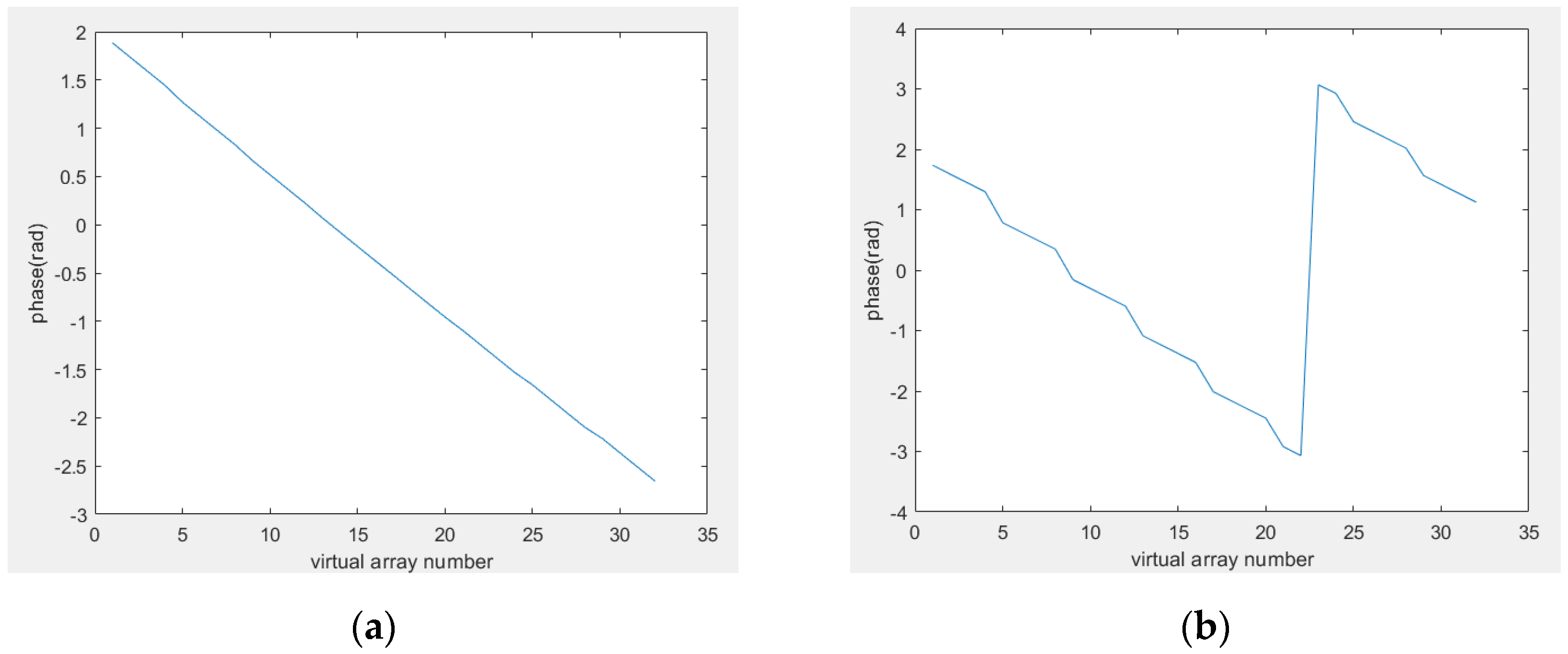
Figure 5.
The matched filter-based imaging scheme with phase compensation.
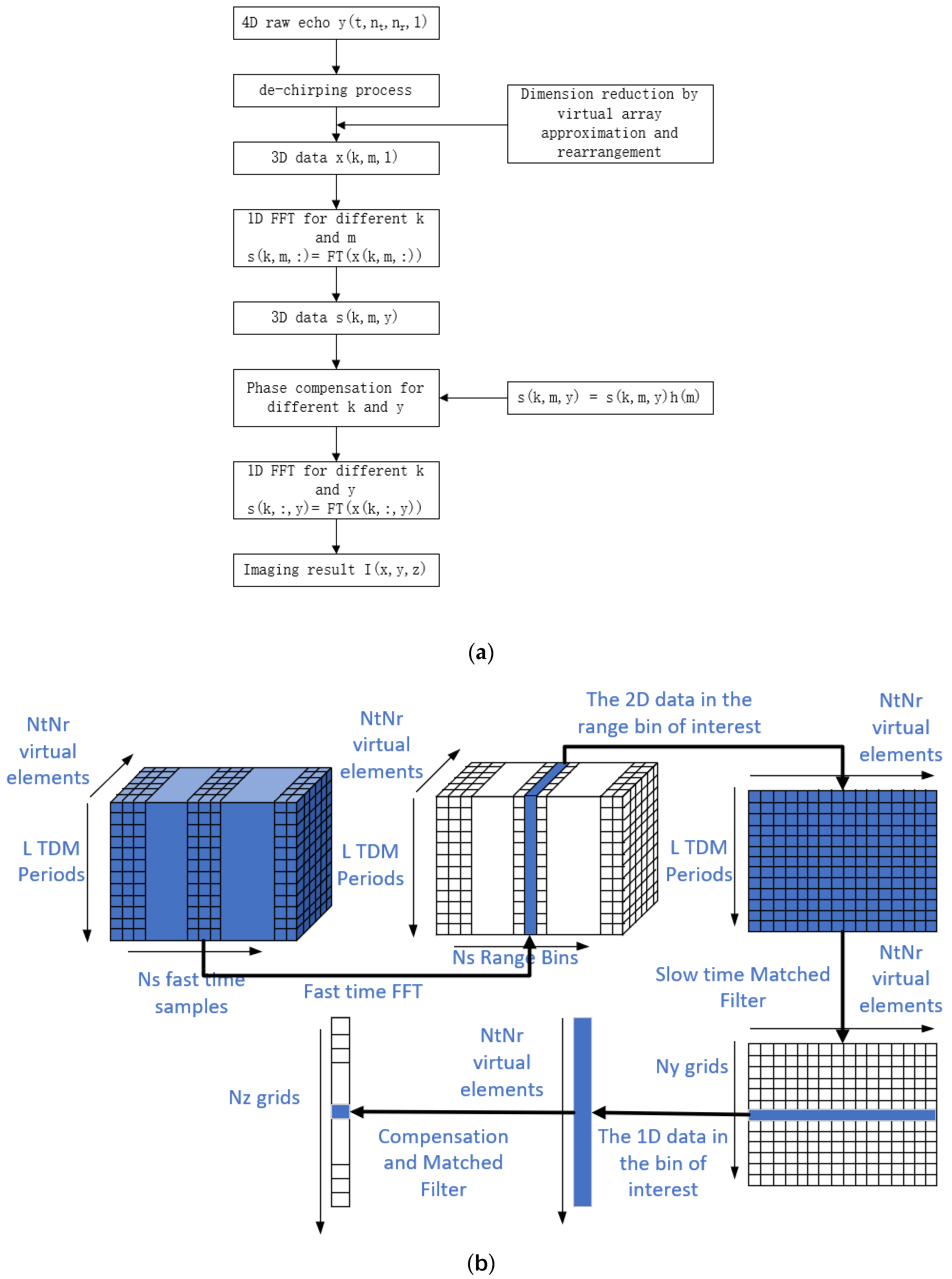
Figure 6.
The simulation result demonstrates how gating lobes affect MIMO-SAR imaging: (a) the 2D projection of the point targets. (b, c, d, e, f) the 2D projection of the 3D MIMO-SAR imaging result following the imaging scheme shown in Table 2. The platform velocity for (b, c, d, e, f) is 3m/s, 5m/s, 10m/s, 20m/s, 25m/s.
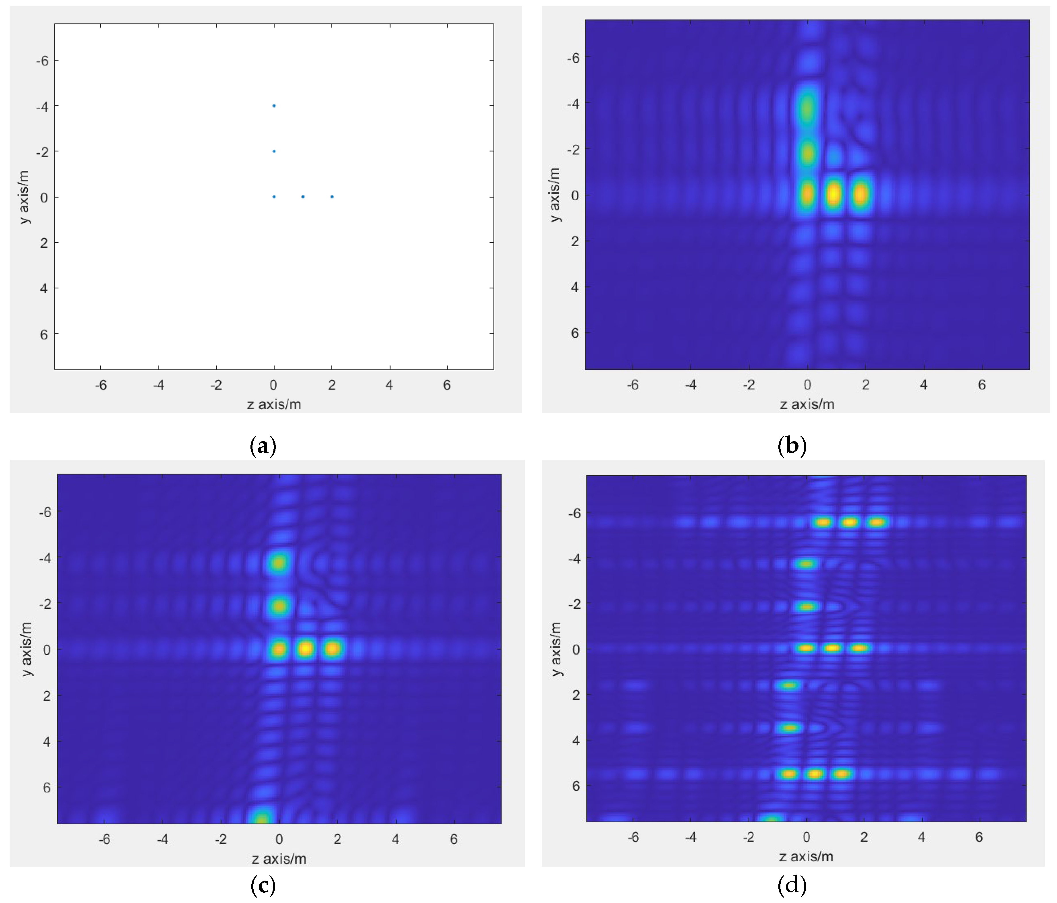
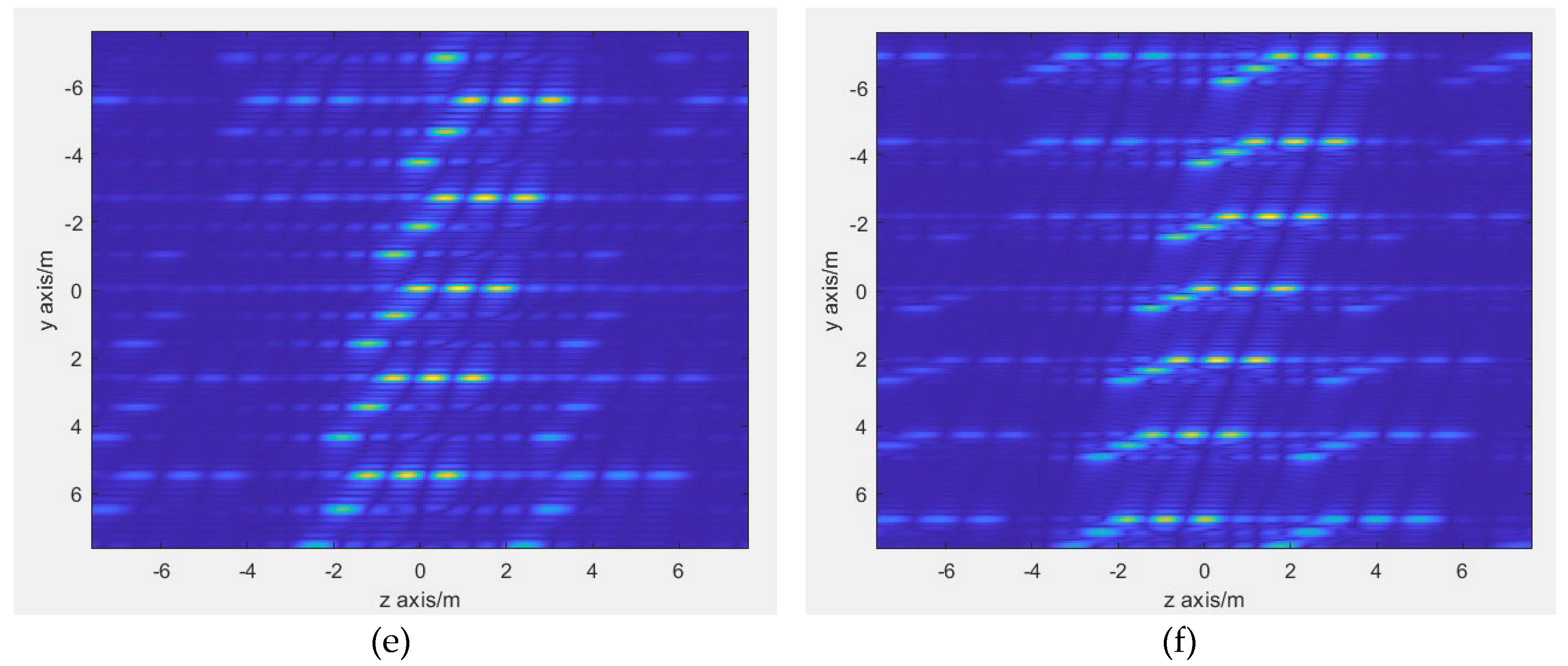
Figure 7.
The simulation results of three targets whose y axis coordinates are 0 m: (a) the 2D-CS process results of gating lobes located at (b) the 2D-CS process results of gating lobes located at . (c) the extracted main diagonal of the 2D-CS process results shown in Figure 7(a). (d) the extracted main diagonal of the 2D-CS process results shown in Figure 7(b).
Figure 8.
The proposed imaging scheme.
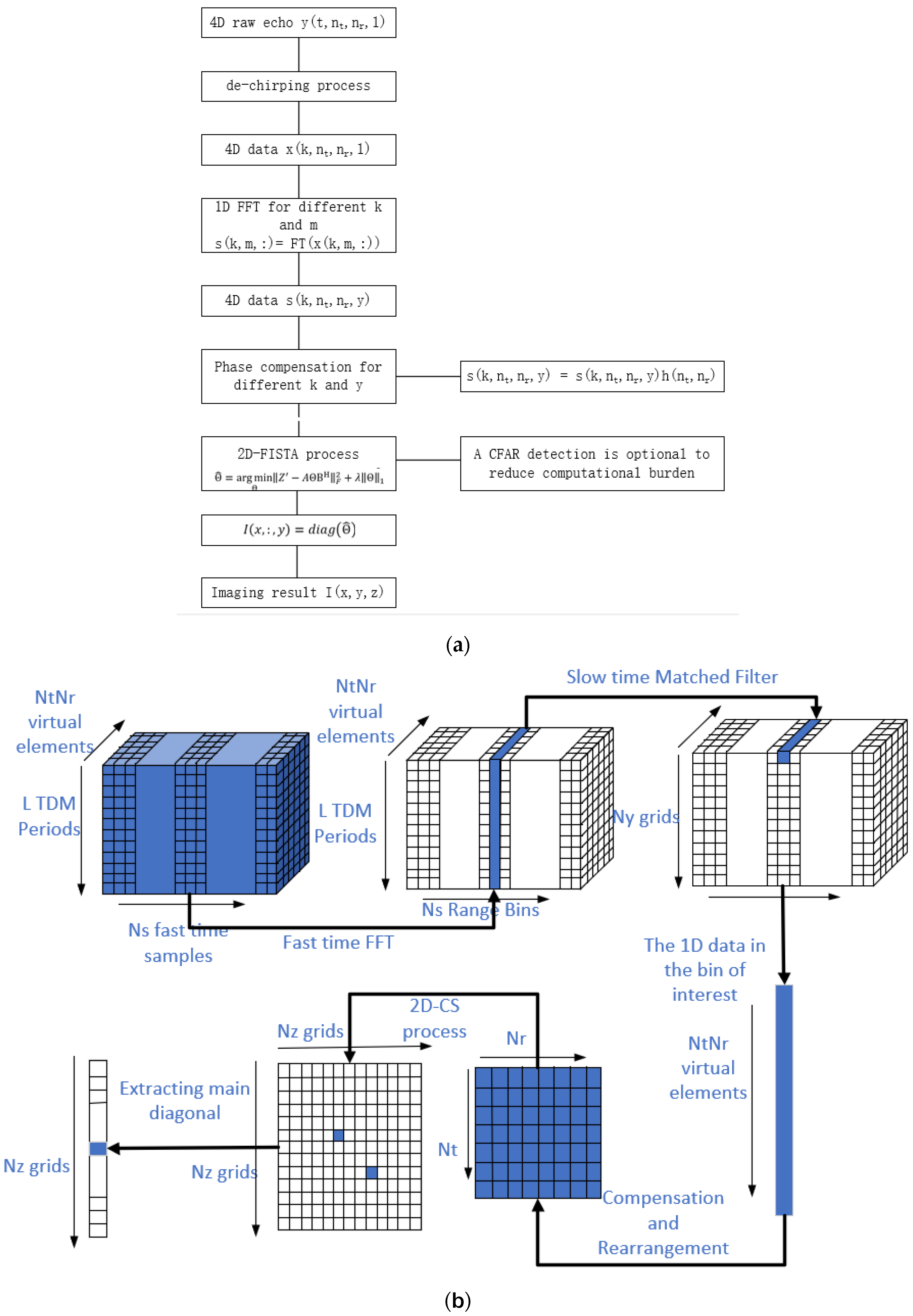
Figure 9.
The simulation results demonstrate the comparison of the MF-based method and the proposed method: (a) the location of the point targets. (b) the 2D projection of point targets. (c, e, g) the 2D projection of the MF-based method imaging results when the platform velocity is [10m/s, 25m/s, 50m/s]. (d, f, h) the 2D projection of the proposed method imaging results when the platform velocity is [10m/s, 25m/s, 50m/s].
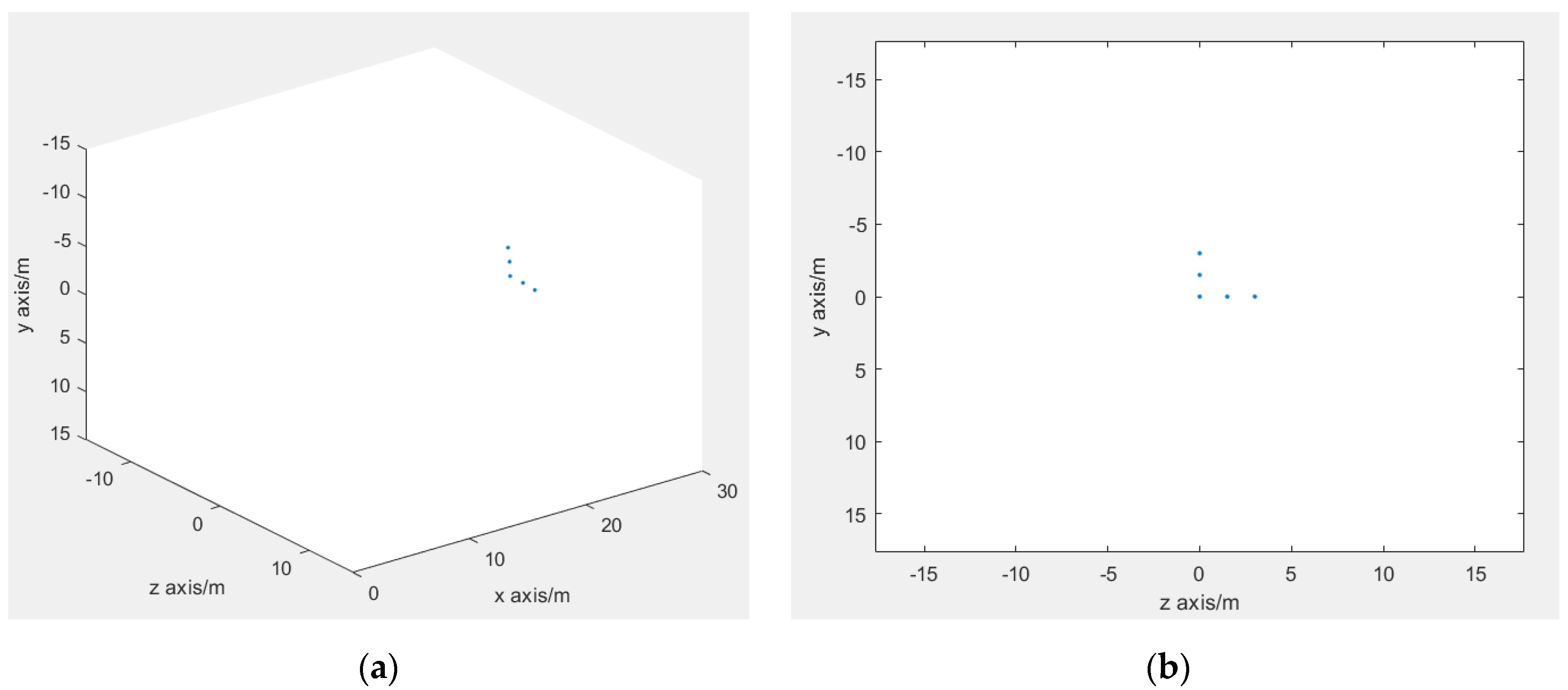
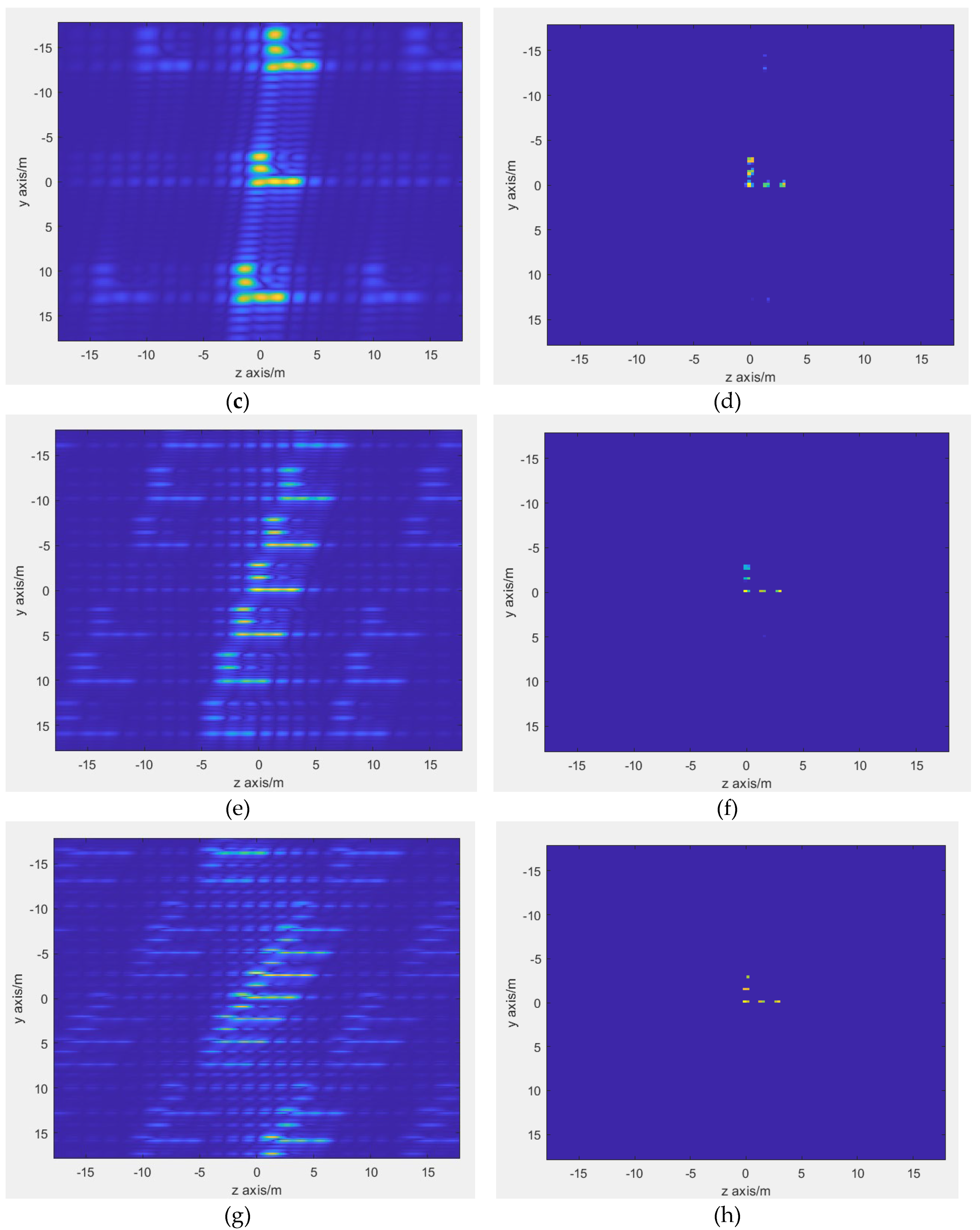
Figure 10.
The simulation results demonstrate the effect of velocity error. The exact speed of the platform is 50m/s: (a) the location of the point targets. (b) the 2D projection of point targets. (c, d, e, f) the 2D projection of the proposed method imaging results with a measured velocity of [50m/s, 47.5m/s, 45m/s, 42.5m/s].
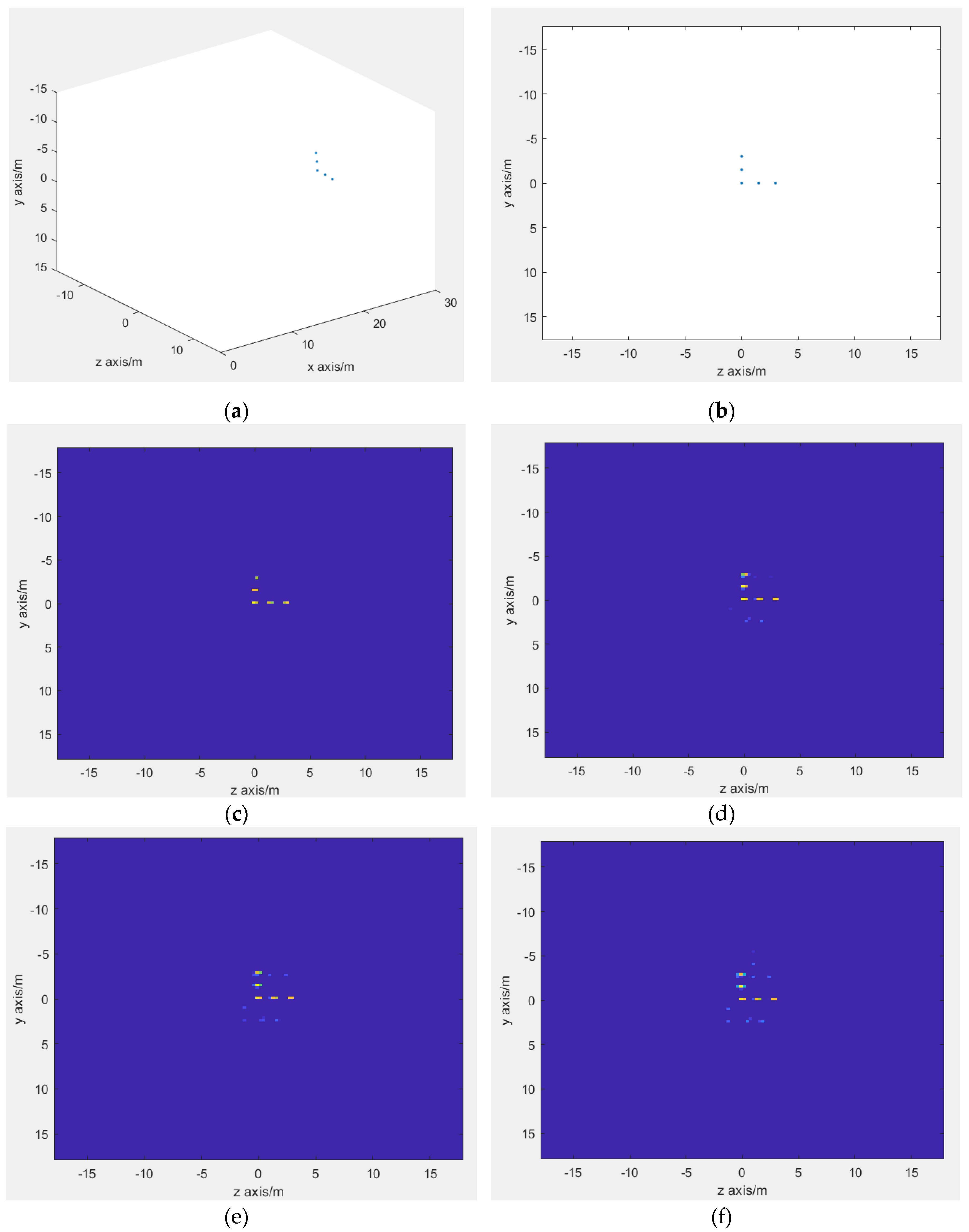
Figure 11.
The structure of antenna elements on AWR2243: (a) a photo of AWR2243 cascaded radar. (b) the structure of AWR2243 antenna elements and chips.
Figure 11.
The structure of antenna elements on AWR2243: (a) a photo of AWR2243 cascaded radar. (b) the structure of AWR2243 antenna elements and chips.
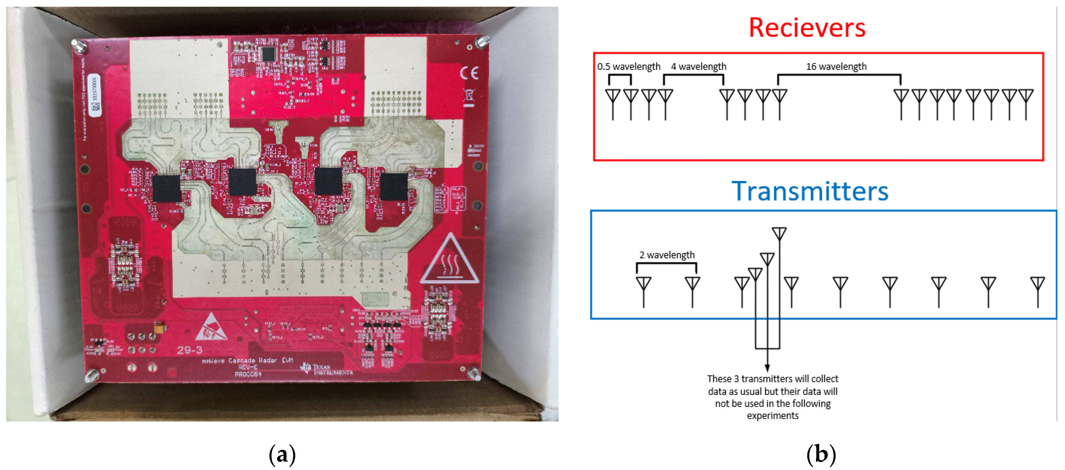
Figure 12.
The experiment setup: (a, b) the AWR2243 MIMO radar is installed on a vehicle which can reach 3m/s. (c) the vehicle is moving straight along a road at maximum speed. (d) three corner reflectors are set by the road. (e) 2D projection of the MF-based algorithm imaging result. (f) 2D projection of the proposed algorithm imaging result.
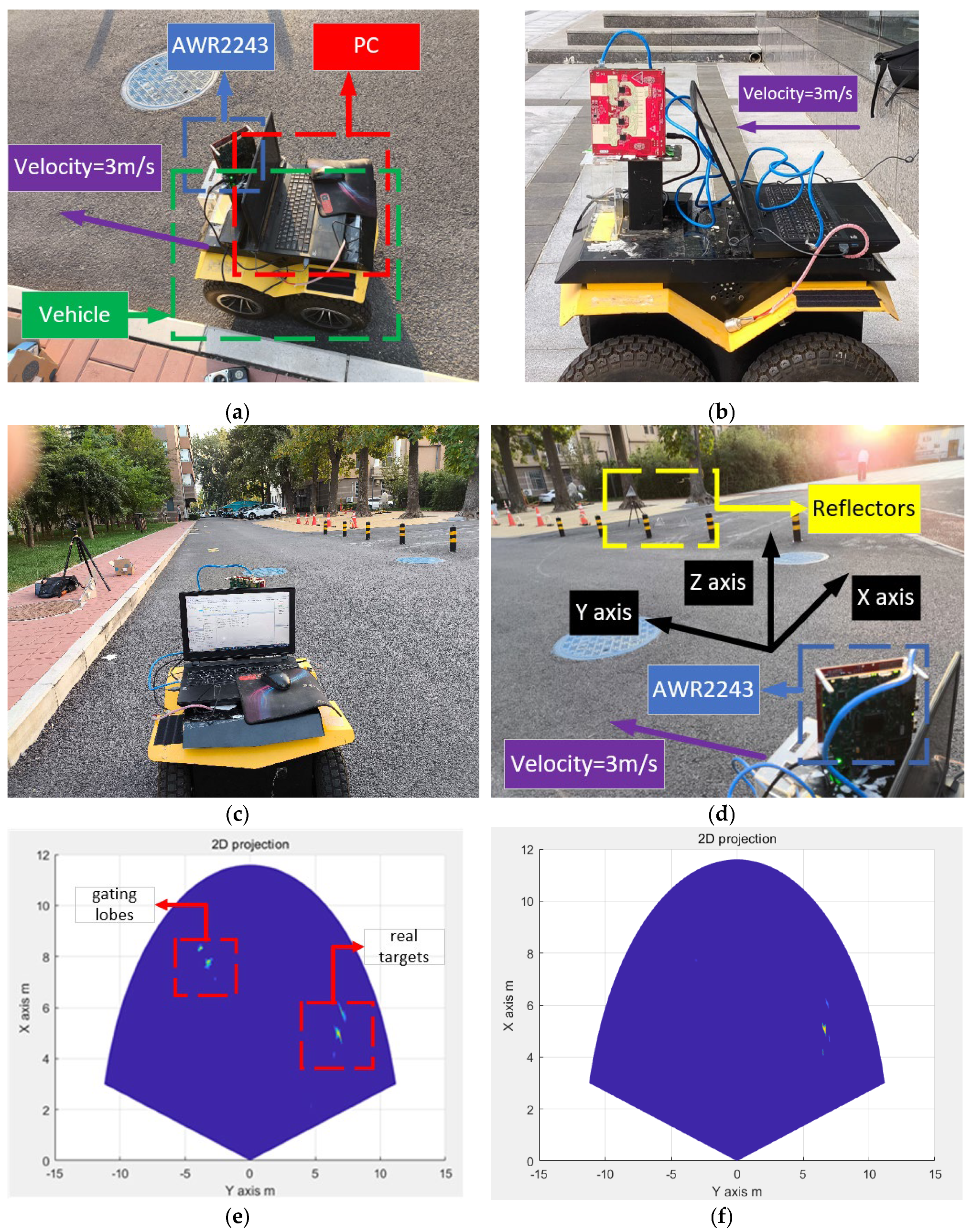
Figure 13.
The experiment setup: (a) the AWR2243 MIMO radar is installed on a car which reach 20km/h. (b) the vehicle is moving straight along a road at 20km/h and the radar is collecting data reflected by the target car. (c) 2D projection of the MF-based algorithm imaging result. (d) 2D projection of the proposed algorithm imaging result.
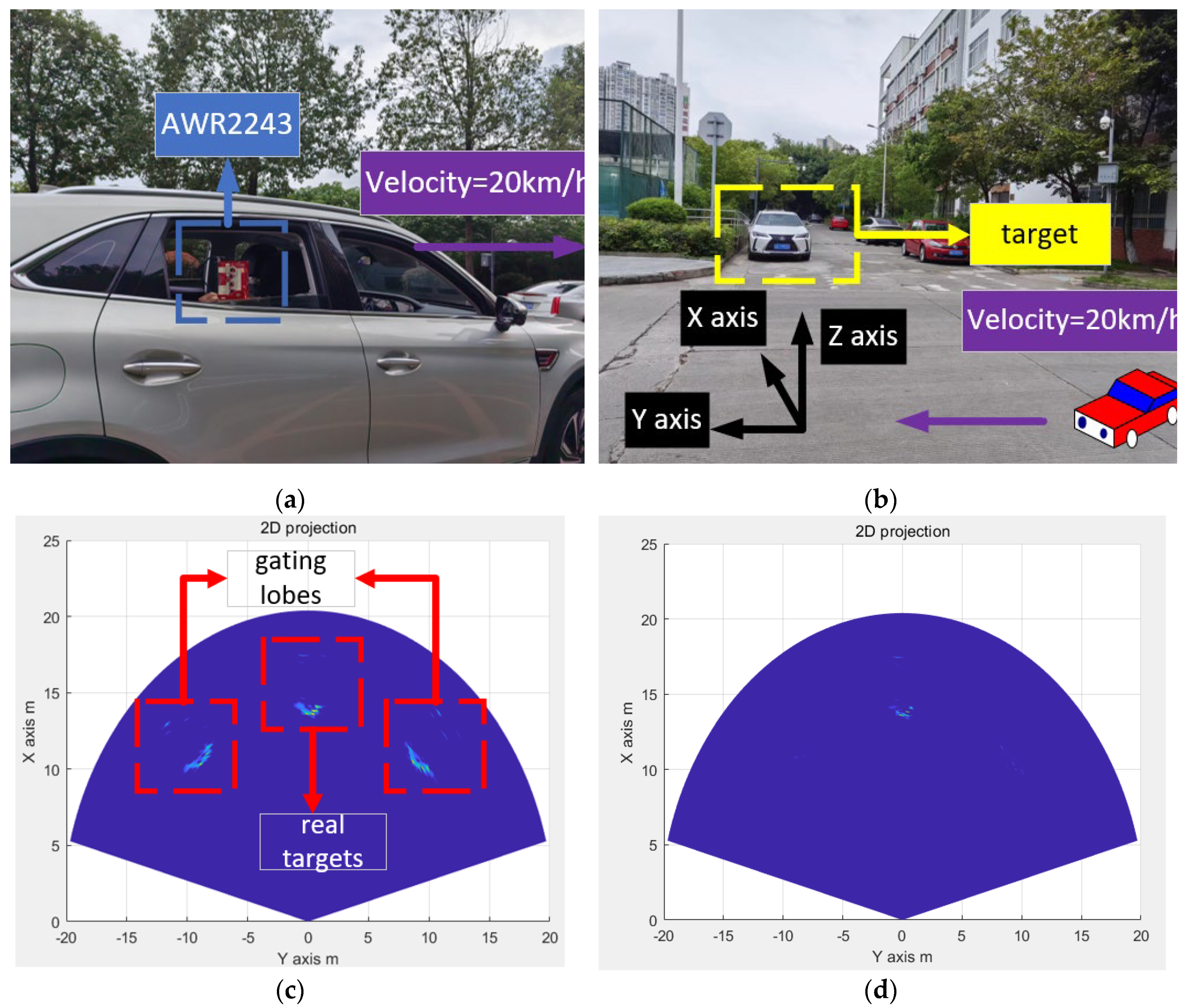

Table 1.
Simulation MIMO radar parameters.
| parameters | |
| 77 GHz | |
| Number of TX | 8 |
| Number of RX | 4 |
| TX spacing | |
| RX spacing | |
| Bandwidth | 160 MHz |
| Pulse Duration | 40us |
| Platform Velocity | 25m/s |
Table 2.
Detailed procedures of the matched filter-based method
| Input: echo signal , number of transmitters , number of receivers , velocity of the platform , the pulse duration , number of TDM periods |
| Step 1. De-chirp the echo signal for every virtual element in every TDM period with equation (6) and (8). . Re-arrange to with equation (14). |
| Step 2. Perform 1D FFT of to .Step 3. Perform phase compensation for with equation (19).Step 4. Perform 1D FFT of to |
| Output: 3D imaging |
Table 3.
Detailed procedure of the FISTA
| Input: measured signal , measurement matrix , , |
| Initiation., , |
| Step k. |
| Output: recovered sparse signal |
Table 4.
Detailed procedure of the 2D-FISTA
| Input: measured 2D signal , measurement matrix , , , |
| Initiation., , |
| Step k. |
| Output: recovered 2D sparse signal |
Table 5.
Detailed procedures of the proposed method
| Input: echo signal , number of transmitters , number of receivers , velocity of the platform , the pulse duration , number of TDM periods |
| Step 1. De-chirp the echo signal for every virtual element in every TDM period with equation (6) and (8). . |
| Step 2. Perform 1D FFT of to .Step 3. Perform phase compensation for with equation (19). Let .Step 4. Perform 2D-FISTA to according to Table 4. The result of 2D-FISTA is denoted as . |
| Step 5. |
| Output: 3D imaging |
Table 6.
Simulation MIMO-SAR parameters.
| Parameters | |
| 77 GHz | |
| 10 MHz | |
| Number of TX | 8 |
| Number of RX | 8 |
| TX spacing | |
| RX spacing | |
| Bandwidth | 160 MHz |
| Pulse Duration | 40us |
| PRI | 320us |
| Number of TDM periods | 16 |
Table 7.
Key parameters of AWR2243.
| Parameters | |
| 77 GHz | |
| 8 MHz | |
| Number of TX | 12 |
| Number of RX | 16 |
| TX Spacing | |
| RX Spacing | |
| Bandwidth | 160 MHz |
| Pulse Duration | 40us |
| Inter-Pulse Idle Time | 5us |
| PRI | 540us |
| Number of TDM periods | 100 |
Disclaimer/Publisher’s Note: The statements, opinions and data contained in all publications are solely those of the individual author(s) and contributor(s) and not of MDPI and/or the editor(s). MDPI and/or the editor(s) disclaim responsibility for any injury to people or property resulting from any ideas, methods, instructions or products referred to in the content. |
© 2024 by the authors. Licensee MDPI, Basel, Switzerland. This article is an open access article distributed under the terms and conditions of the Creative Commons Attribution (CC BY) license (http://creativecommons.org/licenses/by/4.0/).
Copyright: This open access article is published under a Creative Commons CC BY 4.0 license, which permit the free download, distribution, and reuse, provided that the author and preprint are cited in any reuse.


