Submitted:
24 December 2024
Posted:
25 December 2024
Read the latest preprint version here
Abstract
In this study, it was possible to visually check the difference in sound depending on the way the piano key is pressed through the spectrogram. When the keyboard is pressed hard, the high-frequency component is emphasized, and when pressed gently, the low-frequency component is prominent. In addition, it was confirmed that the pattern of the spectrogram varies depending on the playing techniques such as staccato and legato, or whether or not to use the pedal.
We tried to analyze whether the pianist's touch or expressive power could make a difference in the physical wave form, and on the contrary, the pianist was able to accurately infer the connection between the way he played and the sound through the spectrogram.
Keywords:
Waveform
; Piano
; Wavelet Transform
; Spectrogram Analysis
1. Introduction
Pianists and scientists’ views on the principle of how piano sounds are approached from different perspectives. Pianists mainly explain from an artistic, sensory, or empirical perspective, while scientists explain from a physical, acoustical, or engineering perspective [1]. A pianist’s view, which focuses on an artistic perspective, is mainly focused on their performance experience and the expressive power of the sound. Therefore, they understand the piano’s sound by linking it with the emotional elements of tone, touch, pedaling, and performance [2,3]. For example, it emphasizes that the tone changes depending on the pressure and speed of the finger. Pianists see the sound of the piano as an artistic tool rather than a simple mechanical reaction, and they think that pianists convey musical emotions through it [4,5]. Therefore, it is argued that the sound of the piano depends on how the player presses on the keyboard (speed, intensity, touch sensation), which depends on the player’s skill and interpretation [6]. For example, a performer says that even the same note can create a completely different nuance depending on how we make the sound [7]. In addition, pianists recognize that certain pianos (e.g., Steinway, Yamaha) produce a unique sound, which they see as a result of the design of the instrument itself and the interaction of the performer [8,9].
However, scientists analyze piano sound with physical, engineering, and acoustical principles [10]. According to physical principles, the sound of a piano begins when a hammer strikes a string and generates vibrations. This vibrations are amplified through the soundboard, which is then transmitted into the air and heard in the ears. Therefore, the height of a note is determined by the length, thickness, and tension of the piano strings. The magnitude of the sound also depends on the hammer’s strength and hitting speed. To add acoustic analysis to this, piano sound consists of a combination of fundamental frequencies and harmonics. Scientists describe tone as the characteristics of the distribution of sound and resonance, which is an attempt to objectively express a pianist’s sensory explanation. Therefore, even when designing a piano, we focus on creating specific tone and sound characteristics from a mechanical perspective. For example, studying the strength of felt used in hammers or the effect of the material and structure of strings on sound.

Table 1.
Differences in the key perspectives of pianists and physicists
| Pianists | Physicists |
|---|---|
| Focus on the sensory elements and expressiveness of the performance | Focus on the physical/mechanical principles of sound generation |
| Explain that the sound is different by "touch" and "expression" | Explain the difference in sound by the force, speed, and physical |
From a combined point of view, the perspectives of the pianist and the scientist are complementary. The pianist’s experience provides qualitative insights into sound, which can inspire designers or scientists to improve their piano. Scientific analysis also objectively explains the principles of piano sound and can help the performer understand the sound more deeply and develop musical expression based on it. In conclusion, we can best understand the sound and attractiveness of an instrument called a piano when artistic sense and scientific analysis come together.
1.1. History of Piano Timbre
The development of piano and tone has undergone change and growth throughout the centuries as a result of a combination of technological innovation and musical demands. This process has evolved the instrument’s design, material, playing style, and acoustic characteristics [11].
First of all, the piano started in the piano porte, invented by Bartolomeo Cristofori in Italy in the early 18th century. Unlike the existing harpsichord, the piano was able to control the volume (soft and strong sounds) by playing the strings with a hammer. This allowed the performer to play more expressively. The tone was also softer and more delicate than the present on the early piano, and it was suitable for playing in small spaces [12]. Then, with the advent of the classical and romantic era in the 18th and 19th centuries, the technological development of piano and the musical demand rapidly expanded [13].
With the introduction of iron frames in the 1820s, the piano was able to withstand the tension of higher strings, and the sound became louder and richer. The keyboard was also standardized from the existing 5-6 octaves to the current 88 keys (7 octaves), a result of the response to romantic music (e.g., Chopin, Liszt) that required a wider range [11]. In the case of the material of the hammer, it was improved with wool felt, and the arrangement of strings turned into cross-string, providing a resonant tone [14].
As a result of the above, the piano at this time gave off powerful and rich volume, making it suitable for playing in large concert halls. The breadth of musical expression allowed for nuances ranging from delicate tones to intense porte [12].
And with industrialization and mass production in the 20th century, pianos became popular under the influence of the industrial revolution and technological advances. Technically, new materials such as steel strings, solid wood, and high-quality felt are used, durability and sound quality have improved, an upright piano (vertical piano) has been developed to increase space efficiency, and it has become popular for home use. There was also a change in tone, with the spread of popular music and jazz requiring tunes adapted to different music genres. The upright piano preferred a soft and warm tone, while the grand piano preferred a colorful and grand tone [15,16].
In the 21st century, digital technology is contributing greatly to the development of piano and tone. Digital piano and hybrid piano are typical examples [13]. As for the digital piano, it utilizes electroacoustic technology to sample or synthesize piano tones to reproduce them. It is light in weight, does not require tuning, and offers a variety of tones and functions. Hybrid piano combines the structure of acoustic piano with digital technology, providing both traditional tone and modern functionality [17].
The latest digital piano precisely reproduces the sound of a real grand piano using high-quality sampling technology. Physical modeling provides more natural sound by generating virtually the sound of strings and resonators based on acoustic principles. Performers can utilize not only traditional acoustic pianos, but also various digital tones (e.g., electronic pianos, organs, and synthesizers). Technology has enabled the customization of tones.
In conclusion, a wide range of musical genres, from Bach, Beethoven, and Chopin to jazz, pop, and film music, led to the development of the piano’s tone. The performance environment has also improved volume and resonance performance as it has expanded from small-scale salon performances to large concert halls. In terms of technological innovation, technological advances such as iron frames, digital sampling, and physical modeling have improved sound quality and expressiveness. As such, the development of piano and tone has been made through the interaction of music and technology. Early small and delicate tones developed into tones that are magnificent, rich, and suitable for various genres and environments. Through the introduction of digital technology and new materials, piano will continue to provide more innovative tones and evolve.
1.2. The Principle of Piano Sound
The way the piano makes sound basically follows the principle that strings vibrate and sound is transmitted into the air. Specifically, it is as follows:
The piano has several keys, and when the user presses the keys with his finger, the hammer goes up and bounces the strings. Each keyboard is connected to a string that produces a specific sound. Each time the keys are pressed, the strings bounce and the vibration begins [18].
There are also several hammers inside the piano, each of which is connected to a keyboard, and when the keyboard is pressed, the hammer strikes the string and causes vibration. When a hammer hits a string, its sound volume and tone vary depending on its strength and speed. For example, hitting hard and fast makes a loud sound, and hitting slowly by pressing hard makes a small and soft sound [19].
When the hammer hits the strings like this, the strings begin to vibrate quickly. Since the frequencies of each note vary depending on the length, thickness, and material of the strings, each string makes a specific note. There are about 230 strings on a piano, which are arranged in order from low to high. For example, long strings are used for low notes and short and thin strings are used for high notes [20].
Since the sound produced by strings vibrating is a very microscopic sound wave, a resonant container is required for the sound to be heard well by humans. Inside the piano, there is a large wooden box called a resonant container, which amplifies the vibration of the strings even louder. The resonant container diffuses the sound waves generated when strings vibrate, and makes the piano’s sound richer and louder [21].
In addition, the piano has a pedal. There are usually three pedals, which affect the duration and characteristics of the sound. For example, the soft pedal (left pedal) softens the sound by weakening the hit on the strings, and the damper pedal (right pedal) keeps the strings ringing to make the sound last long. Finally, the sound adjustment pedal (center pedal) can fine-tune the length or tone of a sound.
In conclusion, the piano makes a sound when it presses the keyboard and the hammer hits the strings, which are amplified by the resonator. In addition, the characteristics of the sound can be controlled by using pedals.
The graph above visually shows the waveform of sound waves according to the characteristics of the sound:
In loud sound (high amplitude) as Figure 1(a), the amplitude of the waveform is large, and indicates a more intense sound. On the other hand, in small sound (low amplitude) shown in Figure 1(b), the amplitude of the waveform is small, indicating a smooth and quiet sound. Figure 1(c) indicate high sound (high frequency), where the waveform repeats faster and corresponds to a high note. And low-frequency as shown in Figure 1(d) has different waveform which repeats slowly and corresponds to a low-pitched tone [22,23].
1.3. Piano Timbre Analysis from a Physical Point of View
Physically analyzing piano tones is the process of numerically understanding and explaining the characteristics and principles of piano sound using acoustics, physics, and signal processing technology. To first analyze the physical properties of piano tones, we must understand and measure the following factors:
1.3.1. Frequency
The piano notes consist of primary frequencies (basic notes) and several harmonics. The base frequency corresponds to the pitch of a particular keyboard (for example, A4 is 440 Hz), and the background sound is expressed as an integer multiple frequency of this base frequency. The characteristics of the tone depend on the strength and distribution of the tone [24].
1.3.2. Amplitude
The amplitude indicates the magnitude of the sound wave, which determines the volume of the sound. On the piano, the amplitude depends on the strength of the player’s tag [25].
1.3.3. Time Domain
Piano sounds have characteristics that change over time, and the following factors are considered to analyze them: Attack: The part that quickly strengthens when the sound begins. Decay: The process of gradually decreasing the intensity of the sound. Sustain: A sound that is maintained for a certain period of time. Release: The process of sound disappearing completely [26].
1.3.4. Resonance
Piano sounds include resonant effects produced by resonators and strings. Resonance makes the sound richer, and resonance (e.g., symphathic resonance) caused by the interaction of adjacent strings is also analyzed [27].
Here’s how to analyze the piano tone. First, record the piano sound using a microphone and a spectrum analyzer, and then analyze the frequency and amplitude. Recording with a high-quality microphone at this time can increase the accuracy of the sound data. The spectrum is then analyzed, and the intensity of the basic sound and tone is visually identified by converting the sound into the frequency domain. This allows scientists to determine the frequency structure of the tone from a particular keyboard [28].
Fourier Transform is used as a signal processing technique [29]. This is to analyze the sound tone structure and energy distribution by converting signals from Time Domain to Frequency Domain. The results are represented in a spectral graph (indicating the size of each frequency component). Spectrogram also enables dynamic analysis of changes in tone by visualizing the frequency distribution over time [24,30]. For example, to see how the frequency components change while the sound persists or attenuates. A temporal characterization analysis is necessary to measure the amplitude change curve to analyze the temporal characteristics of the piano sound. It graphs the attack, decay, sustain, and release stages of the sound, and calculates the duration and amplitude change rate at each stage. In addition, resonance analysis measures vibration from soundboards and strings, analyzes the effect of piano resonance on tone, and assesses the impact of the acoustic environment on tone by identifying how piano sound is reflected and absorbed in space [29].
Examples of practical application of piano tone analysis in the above way are as follows. First, it is the field of acoustic modeling. It generates a digital model based on the acoustic characteristics of a piano, and mathematically simulates the vibrations of strings and resonators through physical modeling. Modern digital pianos, for example, utilize this model to reproduce the actual piano tone. Second, it can be used for piano design and tuning. The results of the tone analysis are directly used for the design and tuning of the piano. This is because the length, thickness, and tension of the strings are adjusted to implement a specific tone. In addition, the material and hitting strength of the hammer can be reflected in the design. Third, it is possible to analyze the performer’s performance style [31]. It quantitatively analyzes the influence of a performer’s performance style (e.g., strength control, pedaling) through sound data. It analyzes the acoustic differences in how the performer pressed the same keyboard differently. In conclusion, the process of measuring and analyzing various factors, such as frequency, amplitude, temporal characteristics, and resonance, is what physically analyzes the piano tone. This analysis plays a crucial role in piano design, digital acoustic modeling, and performance technique research, contributing to a deeper understanding of the acoustic beauty and technical principles of the piano [32].
2. Methods
2.1. Wavefuction for Physical Analysis
In sound wave analysis, the wave function is used as an important tool to mathematically express and analyze the physical properties of sound waves. Sound waves are essentially vibrations that are transmitted through a medium (air, water, etc.) and can be modeled using the wave function. Below, we will explain how the wave function is used for sound wave analysis [33].
Wave functions are mathematical representations of the dependence of the amplitude, frequency, phase, time, and space of sound waves. Generally, waves are expressed in the following way:
Here, is the value of vibration at the time t and position x (the magnitude of the wave). A is the amplitude of the wave (corresponding to the volume of the sound). expresses wavenumber, the reciprocal of the wavelength (per unit length). means angular frequency, a value associated with the frequency. Lastly, is phase constant, indicating the initial position of the wave. This equation is in the form of a sinusoidal wave, representing a simple model of sound [34].
The use of wave functions in sound wave analysis is crucial because sound wave analysis is a process of understanding the physical and acoustic properties of sound waves by analyzing characteristics such as frequency, amplitude, and phase. Wave functions are used to perform these analyses quantitatively and systematically [35].
Wave functions are transformed into frequency components via Fourier Transform:
Here, represents the spectral intensity of sound waves at frequency f.
This allows us to evaluate the tone by checking the relative intensity of the tone in the piano sound.
However, because Fourier transform does not show how signals change over time, short-time fourier transform(stft) or wavelet transform are used to compensate for this. This method is useful when analyzing how signals change over time.
It is essential when identifying changes in frequency composition over time, for example, such as melodies in music.
The Figure 2 is a schematic representation of the Fourier transform.
Short-time Fourier Transform (STFT) is a very useful tool for analyzing signals in the time-frequency domain, and it is also utilized in music analysis in various ways. STFT divides signals into short time intervals, and performs Fourier transformations on each interval to obtain time and frequency information simultaneously [36,37].
Wavelet Transform, on the other hand, is a time-frequency analysis technique that provides localized time-frequency information of signals in a different way than STFTs in analyzing sound waves (audio signals). While STFT uses a fixed window size, Wavelet Transform analyzes signals while adjusting the window size. This method is particularly powerful for analyzing audio, including abnormal signals (signals whose frequency components vary over time) or short events.
In other words, Wavelet is a short "waveform," a signal that is localized at both frequency and time. Wavelet Transform compares signals to "wavelet functions" at various scales and time locations. Then, at a small scale, we can see the detailed changes with high-frequency components, and at a large scale, we can see the overall structure of the signal with low-frequency components. Therefore, Wavelet Transform performs a multi-resolution analysis of the signal.
Based on the Wavelet Transform results, signals in a specific frequency band can be removed or emphasized, and inverse Wavelet Transform is possible. In addition, the multiscale analysis of signals allows us to analyze the rhythmic structure, so it can be well utilized for the analysis of tone and acoustic features. In particular, Wavelet Transform varies in time-frequency resolution, making it powerful for analyzing abnormal characteristics of signals.
Table 2.
Wavelet Transform versus STFT
| Wavelet Transform | STFT | |
|---|---|---|
| Frequency resolution | High at low frequency, low at high frequency | fixed frequency resolution |
| Time resolution | High at high frequency, low at low frequency | Fixed time resolution |
| Short event analysis | more effective | Relatively less effective |
| Calculation amount | efficient | relatively computationally efficient |
| Application | Abnormal Signal Analysis, Compression, Noise Elimination | Rhythm, Spectrogram Based Analysis |
Wavelet Transform works like a zoom-enabled magnifying glass. This is because it can capture fine details in small areas or the overall outline of a signal in large areas. Because of this, Wavelet Transform excels at analyzing sound waves with fluctuating time-frequency information.
2.2. Spectrogram Analysis
Spectrogram is a tool that visualizes the time, frequency, and amplitude information of a sound at a glance. This allows us to see how the sound changes over time and how strongly a specific frequency band appears.
Data collection must first be preceded in order to analyze music using Spectrogram. In this paper, high-sensitivity microphones are used to record piano sounds and audio interfaces are used for more accurate data.
Now enter the recorded audio data into the spectrogram software to generate the spectrogram. Representative software includes Praat, Sonic Visualizer, MATLAB, Python, and in this paper we used Python.
We can analyze which frequency band appears strongly at a specific time in the spectrogram to check the piano’s harmonics, resonance, and tone change over time.
Window function w(t) is used to highlight or limit specific time intervals in a signal. The selection of window functions affects time and frequency resolutions. Common window functions:
- (1)
- Rectangular window
- (2)
- Hamming Window
- (3)
- Hanning Window:
- (4)
- Gaussian Window:
In Figure 3, we provide Python code used for spectrogram calculation.
Using this, we can visually compare the differences in tone according to various piano models and playing methods. We can also evaluate the harmonious degree of tone by checking the relationship between the fundamental frequency and the tone.
In addition, it is possible to diagnose defects, and if there is a problem with a specific part of the piano (string, hammer, soundboard, etc.), it may appear as an abnormal pattern in the spectrogram. For example, if the tone is murky, the low frequency area is emphasized and the high frequency tone is weak or irregular.
As such, the spectrogram is a powerful tool that allows us to analyze sound objectively, away from simply listening to sound. This allows us to study the tone of various instruments as well as the piano precisely.
2.3. Deep Learning Process
We share the code used for the sound wave prediction model below.
Figure 4.
Deep learning python code for the sound wave prediction model.
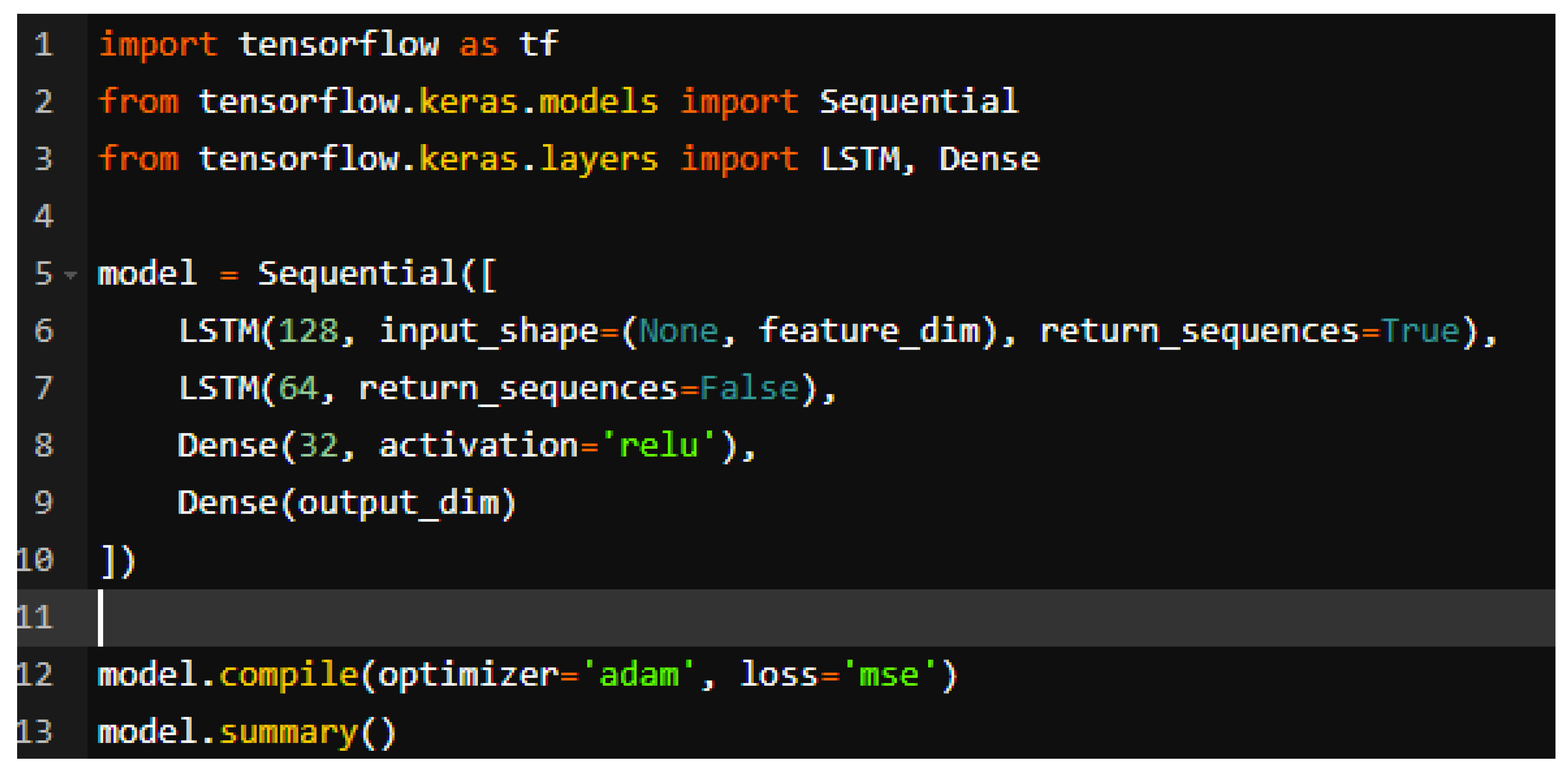
Deep learning can learn high-dimensional, nonlinear relationships directly from sonic data. In particular, piano sound waves contain various elements such as pitch, intensity, rhythm, and combination of chords. Deep learning can automatically analyze and learn these elements, enabling more flexible analysis than traditional signal processing methods.
Traditional methods required a lot of domain knowledge to derive Mel-Frequency Cepstral Coefficient (MFCC), spectrogram, or high-dimensional properties. Deep learning automatically extracts features from raw audio data, thus reducing the process of designing features for manual tasks. Furthermore, deep learning models provide higher accuracy compared to traditional analytical methods, making them robust for dealing with tasks that require fine distinctions, such as piano sound waves (e.g., different touches on the same pitch). By leveraging a large dataset, the models can also learn the personal styles of performers, differences in piano, and environmental noise.
Piano sonic analysis can be learned in combination with score data or performance images, not just by analyzing audio data. For example,
- (1)
- learning sound waves and sheet music at the same time → automatically turning the performance into sheet music (automatic writing).
- (2)
- Learning video data → Analyzing the relationship between the player’s hand movements and sound waves.
As such, deep learning overcomes the limitations of existing signal processing techniques and opens up great possibilities in piano sonar analysis and related applications.
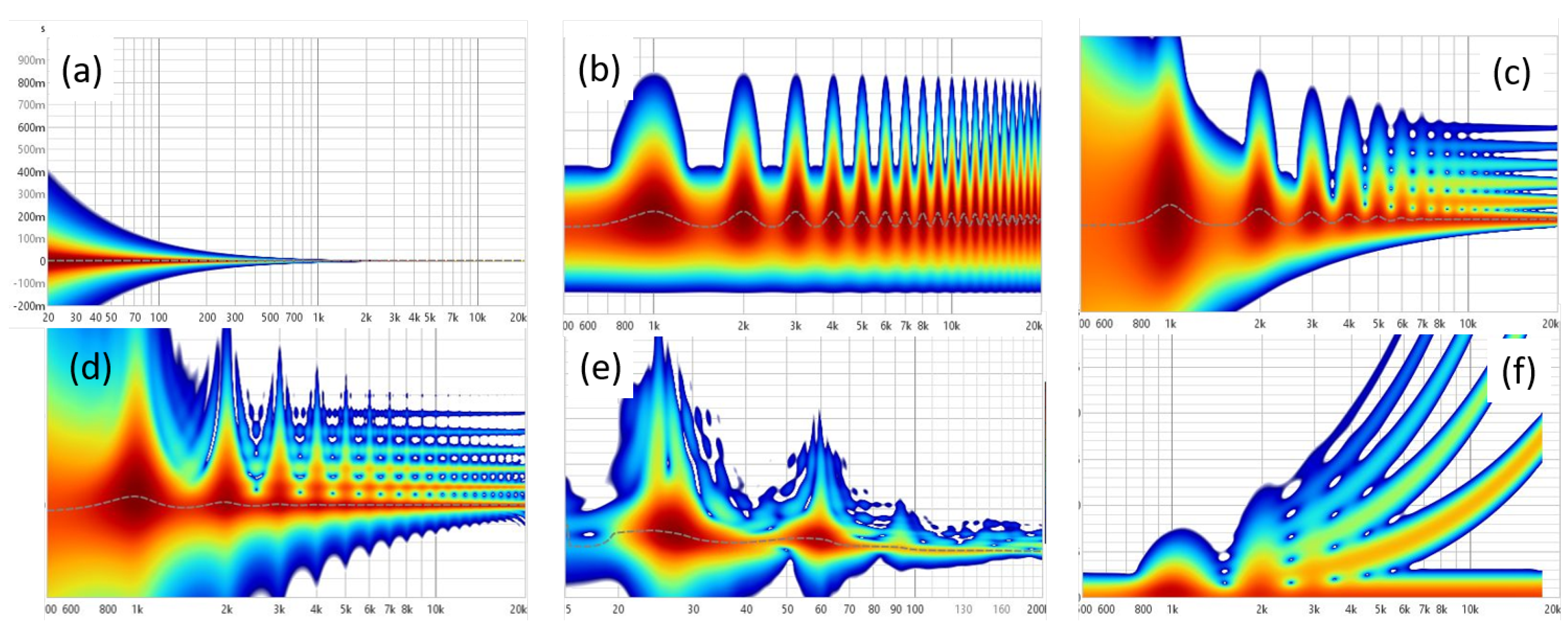
3. Results
The difference in spectograms depending on the touch of the piano keys is mainly due to the strength and skill of the keys, and the position of the keys. A spectogram is a graph that visually represents changes in the frequency and time of a sound, so the difference occurs depending on how the keys are pressed. Some of the key elements are explained below.
First of all, the intensity of the sound varies depending on how hard or gently we press the piano keyboard, and the spectrum varies accordingly. When pressed hard, the high frequency component is more emphasized due to the strong strike, and the dynamic range of the sound is widened. It can react more strongly, especially in the high frequency range. In the spectogram, high frequency is more prominent and strong peaks can be seen as shown in Figure 5(b) while Figure 5(a) shows standard 440 Hz sound. On the other hand, when pressed gently, the sound is relatively smoother and there are fewer high-frequency components. The lower frequency bands (lower frequency ranges) of the spectrum may appear stronger.
The second major element is on articulation. The playing styles such as Staccato and Legato affect the duration and gradation of the sound. For instance, the staccato technique gives each note a short, distinct division. On the spectogram, each note’s duration is short, and the high-frequency component appears to drop quickly as shown in Figure 5(c). Legato, on the other hand, has smooth notes, so continuous frequency changes appear smoother in the spectogram, and the connection between notes appears longer.
The third is the position of the keyboard. In Figure 5(e), we confirm that spectral differences depend on the Bass and Treble regions of the piano, which affect the frequency distribution in the spectrogram. The lower frequency band is emphasized when playing the bass keyboard. The low frequency region is relatively prominent in the spectogram. High-frequency components are emphasized when playing high-pitched keys. In the spectogram, more energy is distributed in the high-frequency domain.
Finally, how to use the pedal is also highlighted in the graph component. The Sustain Pedal allows the sound to persist and multiple notes to ring at the same time. In this case, multiple frequencies overlap in the spectogram, and we can see how the sound continues in a certain pattern as shown in Figure 5(d) and (f). Without the pedal, the note disappears quickly and the spectogram has a shorter negative duration accordingly like Figure 5(a).
In conclusion, the difference in spectograms depending on the touch of the piano keys greatly depends on the strength of the gun, the playing technique, the position of the keys, and whether or not they are used by pedals. This allows to visually analyze the various characteristics of the sound.
Figure 5.
Spectrogram results depending on piano touch.
4. Discussion
In this study, we tried to find connectivity to see if keyboard touch or expressive power, as pianists claim, can directly bring about changes in physical waveforms. As part of that purpose, we introduced the most basic Fourier transform and used spectrograms for visual observation. As a result, it was found that the speed of pressing the keyboard (strength), the acceleration, the position of the keyboard, and the use of the pedal all had a sensitive effect on the results of the spectogram. What was surprising was their answer when they showed the spectogram and asked the pianists, "How do you think you should play the piano for this graph to come out?" Pianists who had little information about how their music was expressed in the physical field were surveyed, but most of them guessed exactly which spectrogram represented how they played. Some musicians gave different answers, but in that case, they were more fascinated by the colorful color than the shape of the wave. When conducting additional surveys, it is necessary to show a black-and-white-toned spectrogram, excluding color.
5. Limitation
Scientific perspectives and calculations on music can help improve the performer’s performance or design the venue, but it is not enough for ’musical impression’. In addition to scientific principles, numerous exercises and personal technical polishing are required to draw the audience’s impression, and the thoughts and attitudes of the performer may be the most important.
For example, when Horovitz returned to his home country for the first time in more than 50 years and played, the audience shed tears of emotion while watching Horovitz playing "Tromerai." Was this because Horovitz impressed with his tremendous tone or because of the sympathy of the audience who knew the footsteps of Horovitz’s life?
Therefore, a scientific approach to music is essential for performers, but they must be aware that it does not always lead to ’musical impression’.
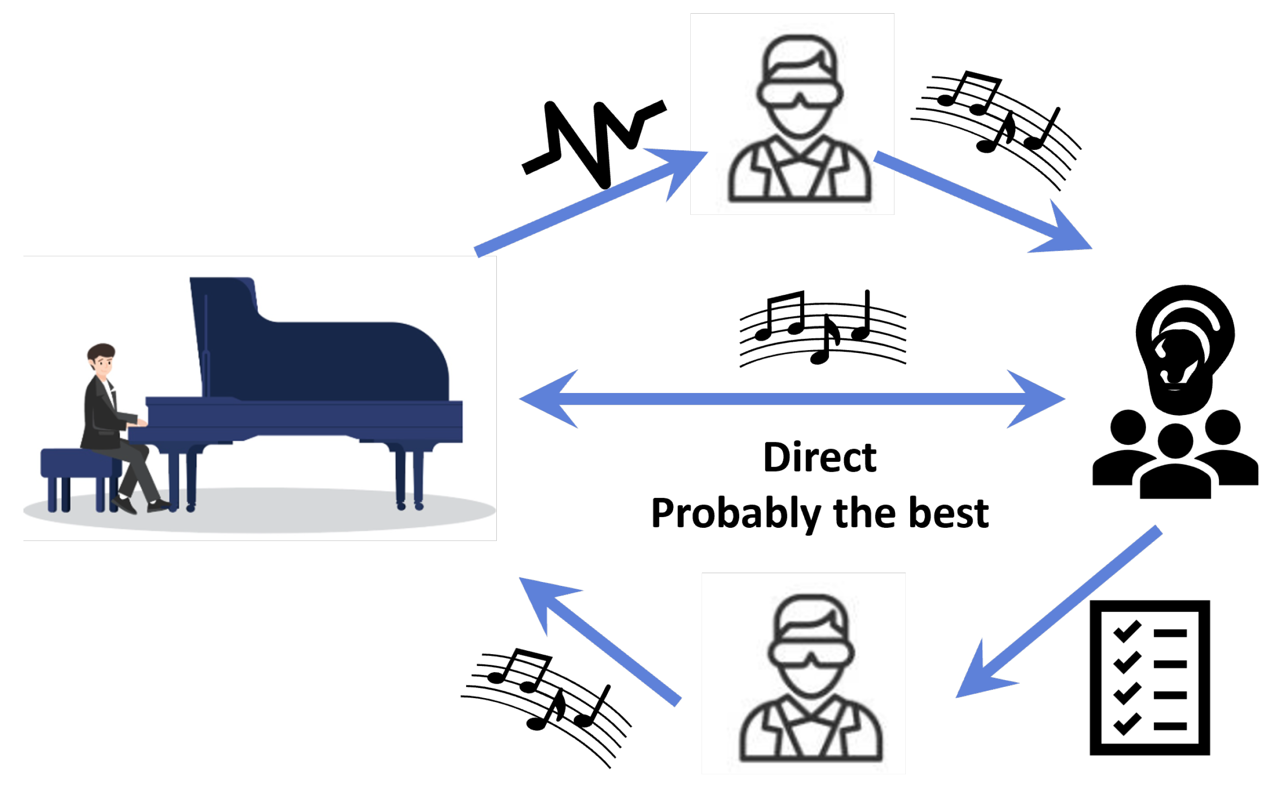
6. Future Work
When working on this paper, the first goal was to see if the performer could analyze piano techniques or emotional expressions in the realm of science, and if possible, how the realm of science could help music. Players have learned that through various techniques, fine movements or expressions can be handled sensitively in the wave graph. On the other hand, if they could understand music by looking at the wave graph, I wondered if hearing-impaired people who could not hear music or those who were in an environment or situation where they could not hear music could also enjoy music through visual information. If the visual sense can give a lingering feeling of the same size as an emotion through hearing, it is expected that scientists’ technology will take a step closer to ’musical emotion’. In the next study, we want to find the role of a scientist from the audience’s point of view rather than the performer’s point of view. Of course, as shown in Figure 6, it is probably the best interaction between the performer and the audience to exchange music as just music. However, even if you look at the basic tuning process, the role of a scientist who analyzes music in waveforms and delivers it is essential. Also, as mentioned above, there is an audience that does not directly receive music. If performers want to convey their musical impression to them, they will need a scientist in the middle.
7. Appendix I
Figure 7.
Piano’s notes with their respective frequencies
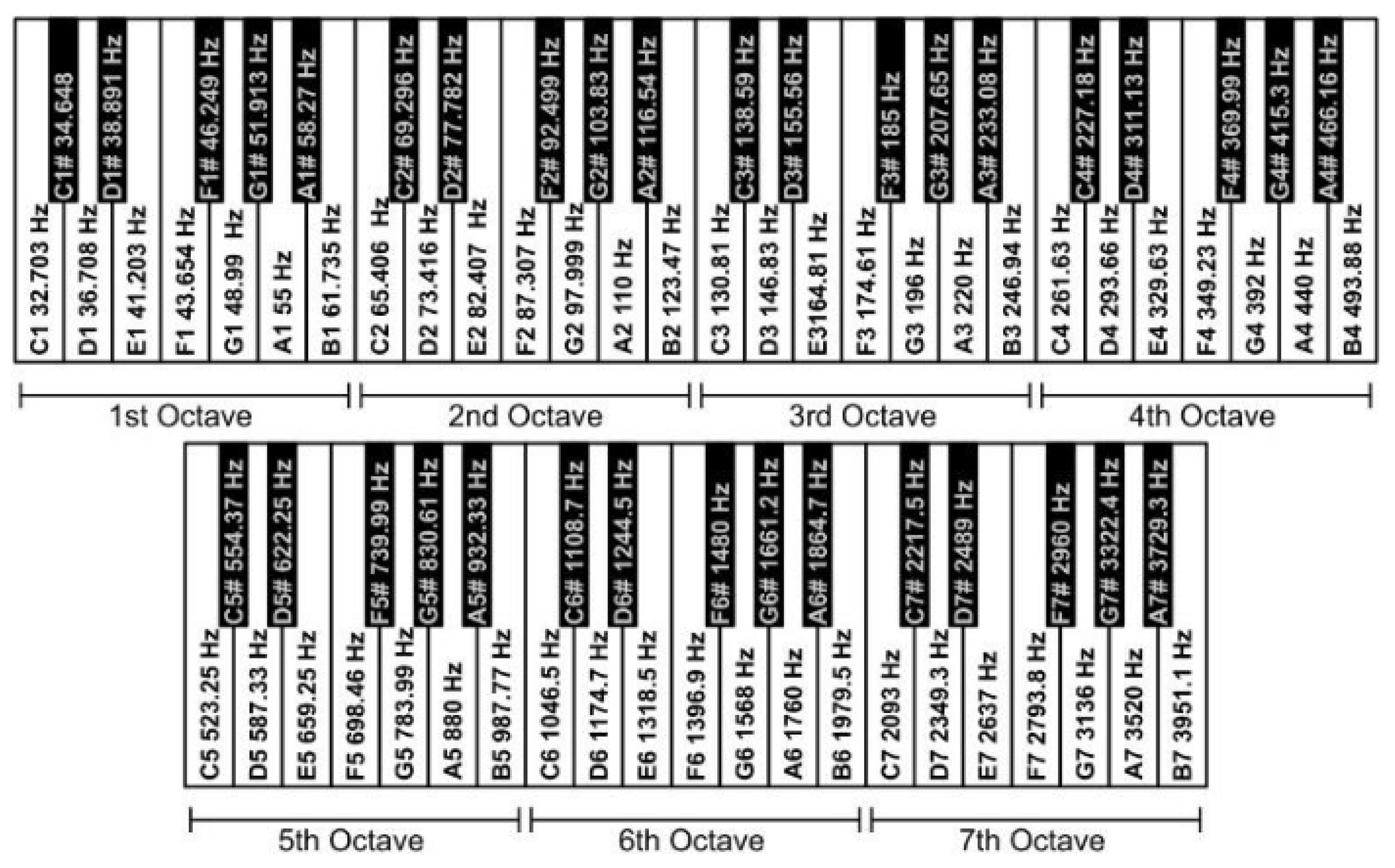
The keys on the piano are divided into seven frequency ranges called "octaves." Each octave exhibits a frequency spectrum twice as large as before. On the piano, each octave is again divided into seven main keys, and each key plays a different note. In classical Western music, in particular, these notes are accompanied by the symbols C, D, E, F, G, A, and B. The frequencies are arranged to increase in alphabetical order. However, contrary to popular opinion, octaves usually start with C and end with B. Since the convention was formed in this manner, the notes are listed semi-alphabetically. The number of cycles per unit time, usually the number of cycles per second, is the frequency of a note, f. Hertz, abbreviated Hz, is a unit of sound frequency that is specified as one cycle per second. As a result, the wave’s frequency is
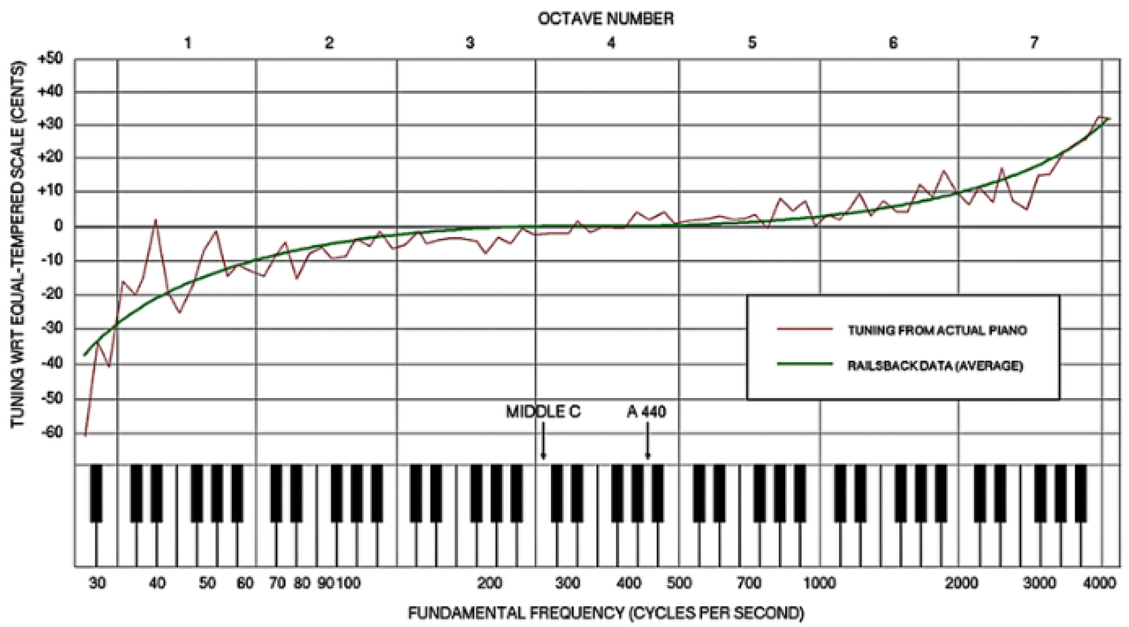
The cacophony varies across instruments, making it difficult to calculate the appropriate stretch with electronic tuning methods. More advanced tuning devices measure individual overtones spectra of all notes and correlate higher harmonics to calculate the required stretch. The latter method yields fairly good results and is increasingly used by professional piano tuners, but many musicians are still convinced that electronic tuning cannot compete with the high-quality auditory tuning of skilled pianos. In fact, when measuring the frequencies of an audibly well-tuned piano, we find that the tuning curves are not smooth. Rather, they exhibit negative to negative irregular fluctuations over the overall elasticity (see Figure 8). At first glance, one might expect that these fluctuations are randomly distributed and are caused by natural inaccuracies in human hearing. However, these fluctuations are probably not entirely random, instead reflecting to some extent the individual irregularities in the overtoned spectrum of each instrument, which could play an important role in high-quality tuning. Perhaps our ears can find better compromises in the very complex space of the spectral lines than most electronic tuning.
Figure 8.
Typical tuning curve of a piano. The plot shows how much the fundamental frequency of each note deviates from the equal-tempered scale. The deviations are measured in cents, defined as 1/100 of a halftone which corresponds to a frequency ratio of 21/1200 ≈ 1.0005778.
Figure 8.
Typical tuning curve of a piano. The plot shows how much the fundamental frequency of each note deviates from the equal-tempered scale. The deviations are measured in cents, defined as 1/100 of a halftone which corresponds to a frequency ratio of 21/1200 ≈ 1.0005778.
8. Appendix II
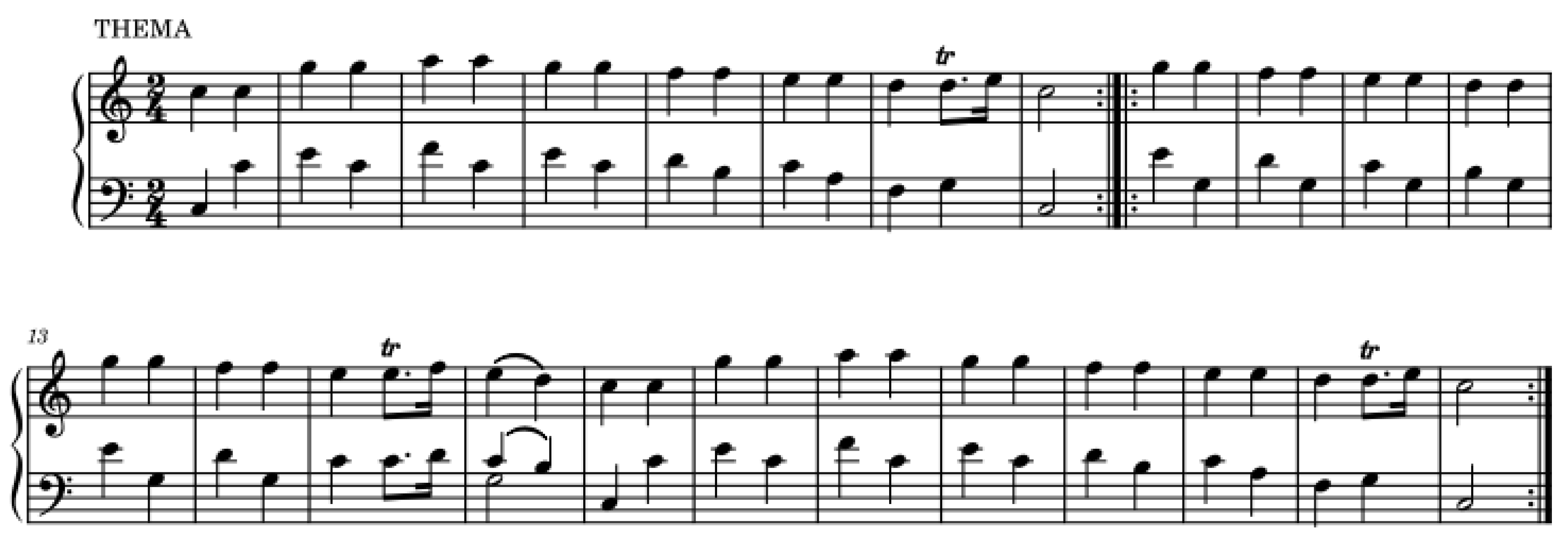
To visually evaluate the accuracy of the results, the score of the song played on the sample is shown in Figure 9. The song is called "Twinkle Twinkle Little Star", which is used for piano learners. The time signature for the music is 4/4. The score is numbered with 12 beats. The score does not have a key signature because the song is in major.
Figure 9.
Sheet music of the song “Twinkle Twinkle Little Star” for sampling.
9. Appendix III
SIGVIEW is a real-time signal analysis application with various spectrum analysis tools, statistical features, and comprehensive graphical analysis methods for 2D and 3D graphics. SIGVIEW analyzes offline or live signals and has a variety of analysis tools, allowing researchers to focus on practical scientific phenomenon analysis instead of learning to use the program.
Just like how a standard calculator processes numerical representations, SIGVIEW’s embedded signal calculator facilitates combinations of signals or instruments through various arithmetic or signal analysis tasks. This tool can be used to perform various cross-spectrum analyses, such as adding or subtracting two signals or spectra.
Each change in the signal will cause the spectrum to be calculated again. A single spectrum will be calculated from the complete visible signal part of the source window. This is the default behaviour as shown in Figure 10.
Figure 10.
Spectral Analysis Defaults
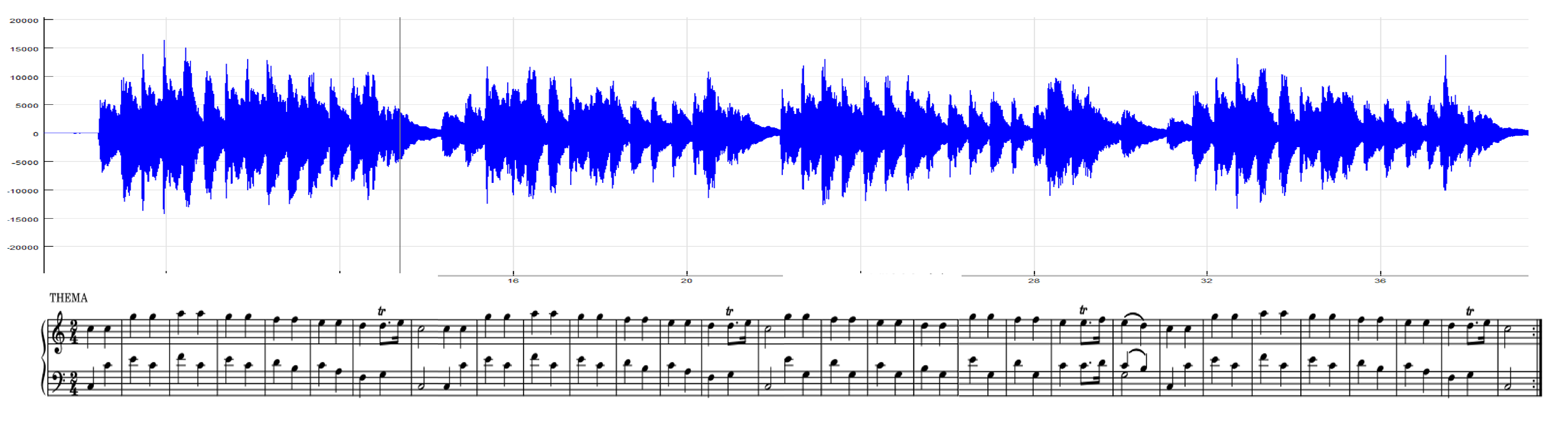
Figure 11.
2D signal filter.
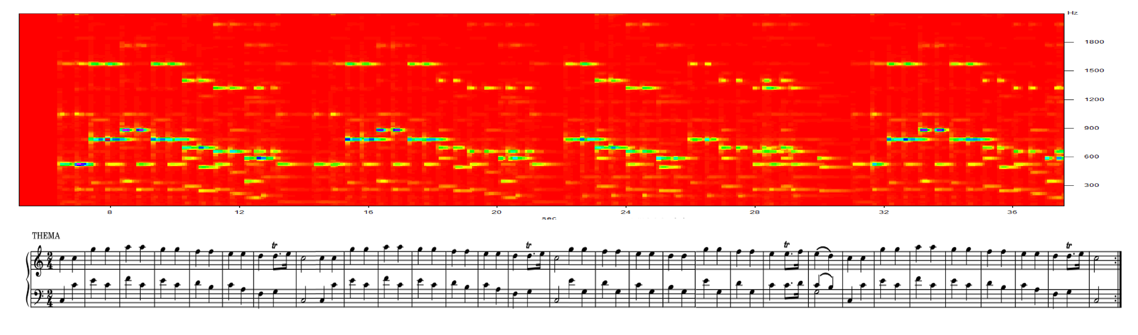
Figure 12.
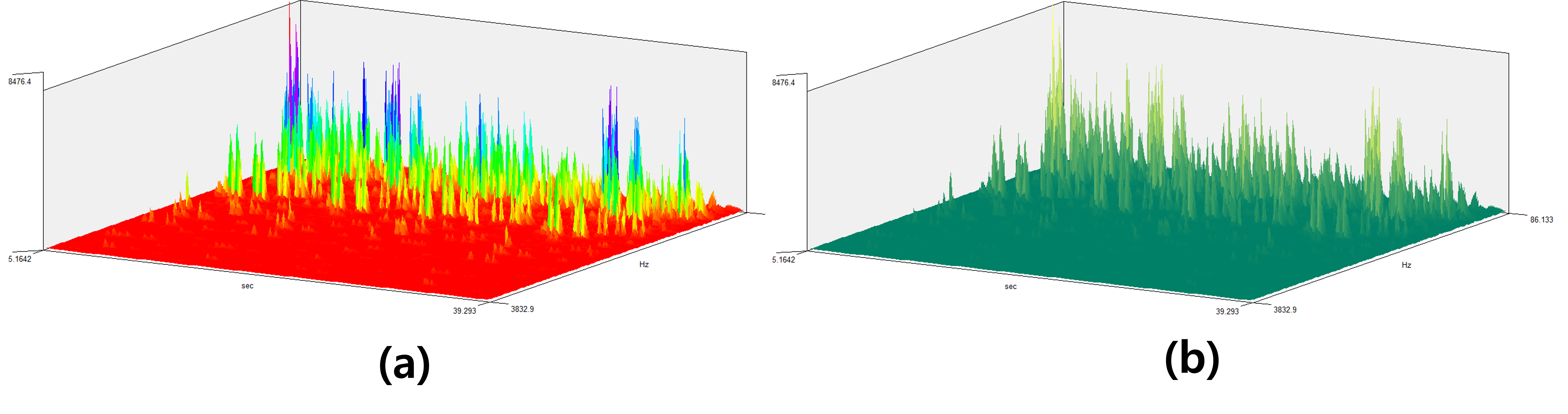
3D signal filter. (a) Colored and (b) One tone type
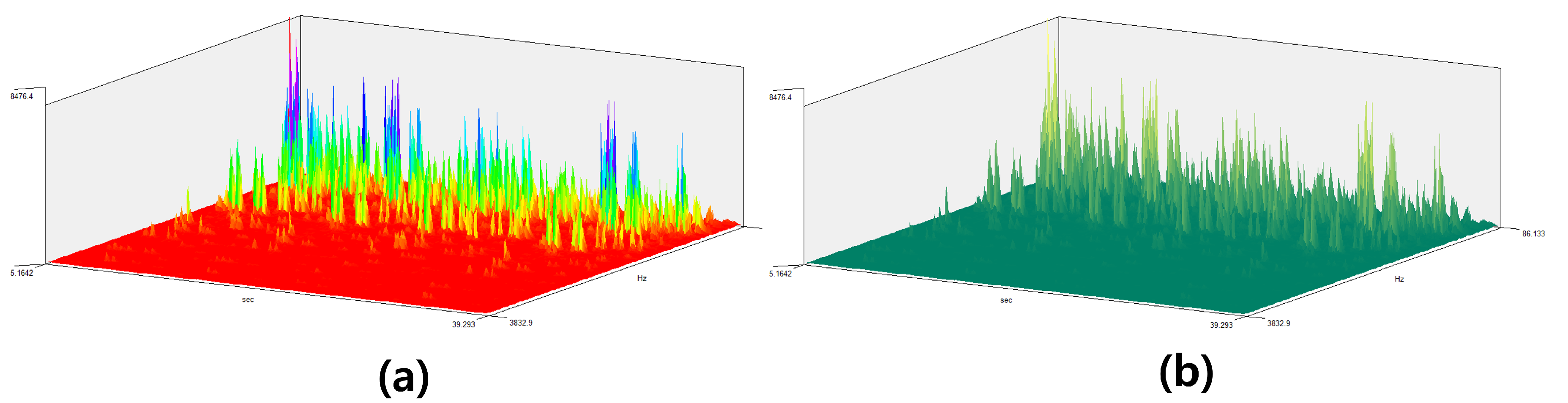
If you need to apply a complex set of filters with different time/frequency ranges and amplitudes to the signals, you can use the ’3D signal filter’ function. The filter characteristics can be defined in three dimensions: time, frequency, and amplitude, hence the name ’3D’.
References
- Bank, B.; Avanzini, F.; Borin, G.; De Poli, G.; Fontana, F.; Rocchesso, D. Physically informed signal processing methods for piano sound synthesis: a research overview. EURASIP journal on advances in signal processing 2003, 2003, 1–12. [Google Scholar] [CrossRef]
- Bank, B.; Sujbert, L. Generation of longitudinal vibrations in piano strings: From physics to sound synthesis. The Journal of the Acoustical Society of America 2005, 117, 2268–2278. [Google Scholar] [CrossRef] [PubMed]
- Blackham, E.D. The physics of the piano. Scientific american 1965, 213, 88–99. [Google Scholar] [CrossRef]
- Giordano, N.J. Physics of the Piano; Oxford University Press, 2010. [Google Scholar]
- Kochevitsky, G. The art of piano playing: A scientific approach; Alfred Music, 1995. [Google Scholar]
- Kulcsár, D.; Fiala, P. A compact physics-based model of the piano. Proceedingd of DAGA 2016. [Google Scholar]
- Rauhala, J.; et al. Physics-Based Parametric Synthesis of Inharmonic Piano Tones; Helsinki University of Technology, 2007. [Google Scholar]
- Simionato, R.; Fasciani, S.; Holm, S. Physics-informed differentiable method for piano modeling. Frontiers in Signal Processing 2024, 3, 1276748. [Google Scholar] [CrossRef]
- Stulov, A. Physical modelling of the piano string scale. Applied Acoustics 2008, 69, 977–984. [Google Scholar] [CrossRef]
- Xie, H. Physical Modeling of Piano Sound. arXiv 2024, arXiv:2409.03481. [Google Scholar] [CrossRef]
- Wagner, E. History of the Piano Etude. The American Music Teacher 1959, 9. [Google Scholar]
- Bartels, A. A HISTORY OF CLASS PIANO INSTRUCTION. Music Journal 1960, 18, 42. [Google Scholar]
- Russo, M.; Robles-Linares, J.A. A Brief History of Piano Mechanics. In Advances in Italian Mechanism Science: Proceedings of the 3rd International Conference of IFToMM Italy; Springer, 2021; pp. 11–19. [Google Scholar]
- Newman, W.S. A Capsule History of the Piano. The American Music Teacher 1963, 12, 14. [Google Scholar]
- HG. History of the Piano, 1948.
- Russo, M.; Robles-Linares, J.A. A Brief History of Piano Action Mechanisms. Advances in Historical Studies 2020, 9, 312–329. [Google Scholar] [CrossRef]
- Tomes, S. The Piano: A History in 100 Pieces; Yale University Press, 2021. [Google Scholar]
- Story, B.H. An overview of the physiology, physics and modeling of the sound source for vowels. Acoustical Science and Technology 2002, 23, 195–206. [Google Scholar] [CrossRef]
- Linder, C.J.; Erickson, G.L. A study of tertiary physics students’ conceptualizations of sound. International Journal of Science Education 1989, 11, 491–501. [Google Scholar] [CrossRef]
- Bennet-Clark, H.C. Songs and the physics of sound production. Cricket behavior and neurobiology 1989, 227–261. [Google Scholar]
- Josephs, J.J.; Slifkin, L. The physics of musical sound. Physics Today 1967, 20, 78–79. [Google Scholar] [CrossRef]
- Sataloff, J.; Sataloff, J. The Physics of Sound. 2. Hearing Loss 2005, 2. [Google Scholar]
- Daschewski, M.; Boehm, R.; Prager, J.; Kreutzbruck, M.; Harrer, A. Physics of thermo-acoustic sound generation. Journal of applied Physics 2013, 114. [Google Scholar] [CrossRef]
- Wever, E.G.; Bray, C.W. The nature of acoustic response: The relation between sound frequency and frequency of impulses in the auditory nerve. Journal of experimental psychology 1930, 13, 373. [Google Scholar] [CrossRef]
- Mellinger, D.K. Feature-Map Methods for Extracting Sound Frequency Modulation. In Conference Record of the Twenty-Fifth Asilomar Conference on Signals, Systems & Computers; IEEE Computer Society, 1991; pp. 795–796. [Google Scholar]
- Wood, J.C.; Buda, A.J.; Barry, D.T. Time-frequency transforms: a new approach to first heart sound frequency dynamics. IEEE Transactions on Biomedical Engineering 1992, 39, 730–740. [Google Scholar] [CrossRef]
- Hawk, B. Sound: Resonance as rhetorical. Rhetoric Society Quarterly 2018, 48, 315–323. [Google Scholar] [CrossRef]
- Flax, L.; Dragonette, L.; Überall, H. Theory of elastic resonance excitation by sound scattering. The Journal of the Acoustical Society of America 1978, 63, 723–731. [Google Scholar] [CrossRef]
- Bracewell, R.N. The fourier transform. Scientific American 1989, 260, 86–95. [Google Scholar] [CrossRef] [PubMed]
- Williams, E.G. Fourier acoustics: sound radiation and nearfield acoustical holography; Academic press, 1999. [Google Scholar]
- Yoganathan, A.P.; Gupta, R.; Udwadia, F.E.; Wayen Miller, J.; Corcoran, W.H.; Sarma, R.; Johnson, J.L.; Bing, R.J. Use of the fast Fourier transform for frequency analysis of the first heart sound in normal man. Medical and biological engineering 1976, 14, 69–73. [Google Scholar] [CrossRef]
- Hornikx, M.; Waxler, R.; Forssén, J. The extended Fourier pseudospectral time-domain method for atmospheric sound propagation. The Journal of the Acoustical Society of America 2010, 128, 1632–1646. [Google Scholar] [CrossRef] [PubMed]
- Tohyama, M. Waveform Analysis of Sound; Springer, 2015. [Google Scholar]
- Westervelt, P.J. Scattering of sound by sound. The Journal of the Acoustical Society of America 1957, 29, 199–203. [Google Scholar] [CrossRef]
- Dean III, L.W. Interactions between sound waves. The Journal of the Acoustical Society of America 1962, 34, 1039–1044. [Google Scholar] [CrossRef]
- Maas, T. Sound Analysis using STFT spectroscopy. Bachelor Thesis, University of Bremen, 2011; pp. 1–47. [Google Scholar]
- Lee, J.Y. Sound and vibration signal analysis using improved short-time fourier representation. International Journal of Automotive and Mechanical Engineering 2013, 7, 811–819. [Google Scholar] [CrossRef]
Figure 1.
Change in sound according to waveform
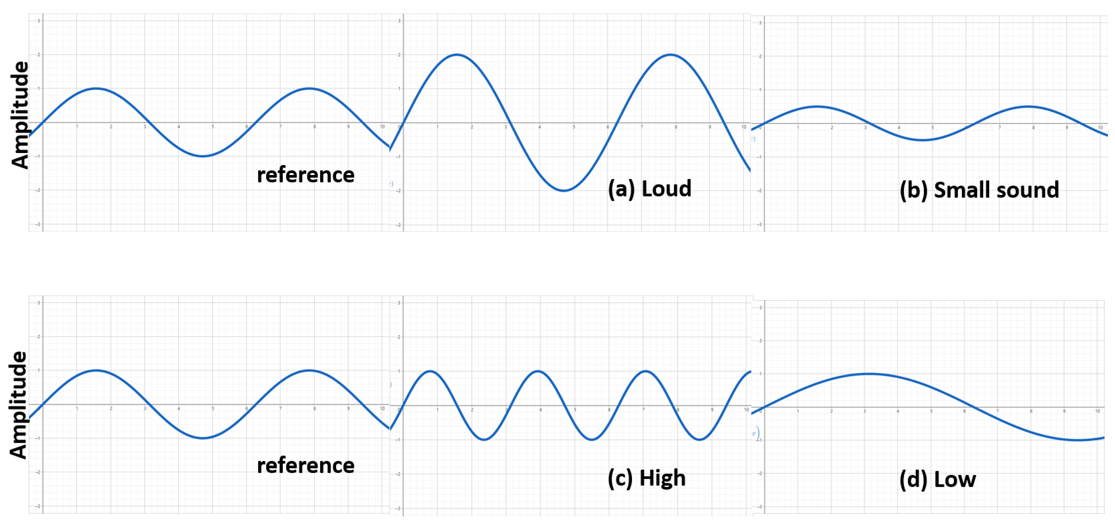
Figure 2.
Schematic representation of the Fourier transform.
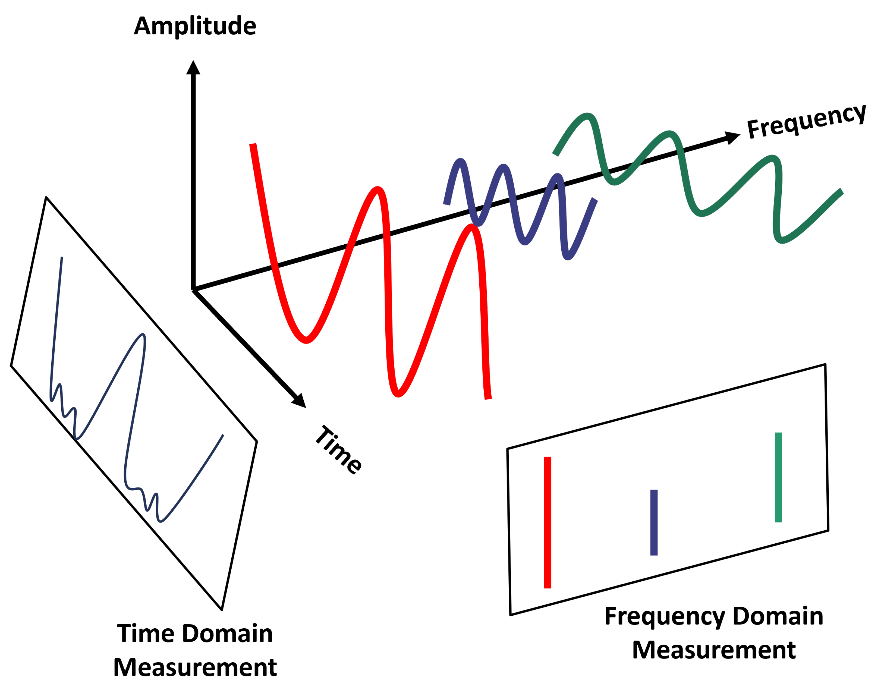
Figure 3.
Python code used for spectrogram calculation.
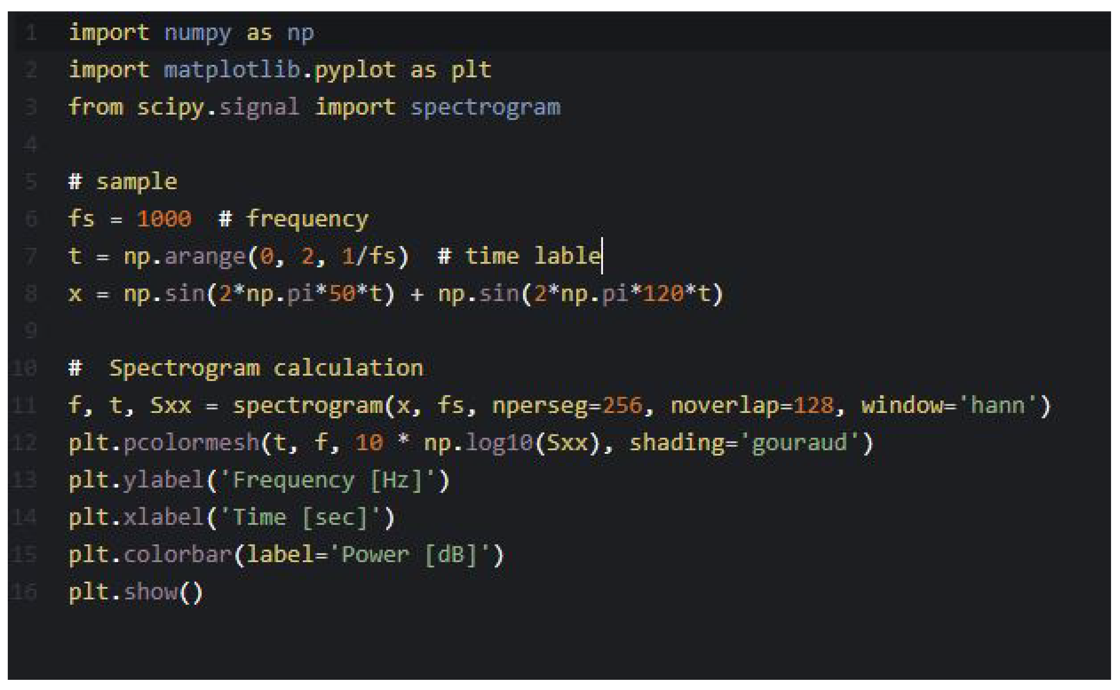
Figure 6.
A schematic diagram of the role between the performer, the audience, and the scientist.
Disclaimer/Publisher’s Note: The statements, opinions and data contained in all publications are solely those of the individual author(s) and contributor(s) and not of MDPI and/or the editor(s). MDPI and/or the editor(s) disclaim responsibility for any injury to people or property resulting from any ideas, methods, instructions or products referred to in the content. |
© 2024 by the authors. Licensee MDPI, Basel, Switzerland. This article is an open access article distributed under the terms and conditions of the Creative Commons Attribution (CC BY) license (http://creativecommons.org/licenses/by/4.0/).
Copyright: This open access article is published under a Creative Commons CC BY 4.0 license, which permit the free download, distribution, and reuse, provided that the author and preprint are cited in any reuse.


