
Submitted:
20 December 2024
Posted:
23 December 2024
You are already at the latest version
Abstract
Biaxial quasistatic MEMS micro mirrors can be used in vector scanning applications to arbitrarily direct a laser beam towards a target in a step-and-settle operating mode, or to follow a setpoint signal in a tracking mode. However, MEMS structures are typically underdamped mass-spring systems - any transient excitation results in a slowly decaying oscillation. Actuators based on sputtered AlScN allow for computationally efficient open-loop control due to the inherently linear piezoelectric properties of the material over a wide operating range. We demonstrate this using a real-time tunable digital filter design based on the inversion of a second order transfer function. This approach effectively reduces the decay time to the millisecond range.
Keywords:
microscanner
; MEMS
; MOEMS
; open-loop control
; quasistatic actuation
; residual oscillation
; piezoelectric actuator
; AlScN
; rapid control prototyping
; MATLAB
1. Introduction
Quasistatic micro mirrors can be used for vector scanning in applications like metrology, laser machining or optical communication. By vector scanning, we mean the arbitrary positioning of a laser beam in a step-and-settle mode or by smoothly tracking a position setpoint signal. Potential application examples are LIDAR or triangulation-based distance measurement, additive manufacturing or laser gravure and optical free-space communication.
The MEMS technology (micro-electro-mechanical system) with its planar lithography techniques on the wafer level produces such devices in small size and its mass production capability makes them equally suitable for industrial, automotive or consumer markets. Given the bearing-less construction of MEMS scanners, they are ideal candidates for vacuum environments like in quantum technology or space application. However, with springs and masses being the only construction elements, one has to deal with resonant modes of the underdamped structure: Any transient excitation causes long-lasting oscillations in various parts of the mechanics. Adding physical viscous damping elements, if technologically feasible, would significantly reduce the usable bandwidth of the system. A more efficient approach is to shape input signals in a way that avoids resonant excitation. The most versatile technique for this purpose is the use of digital filters. In this paper, we want to show how a simple realization of an open-loop control algorithm can reduce the settling time of a gimbal-less, biaxial, quasistatic MEMS micro mirror with piezoelectric Aluminium-Scandium-Nitride (AlScN) actuators by a factor of one thousand. Although such an open-loop control is clearly not capable of suppressing the effects of exogeneous excitation by shock or vibration, it already addresses the needs of many applications and shows the principal dynamic capabilities of the device.
The algorithm presented here targets controller platforms with limited resources, like many microcontrollers or embedded systems with spare processing resources. We used a Rapid-Control Prototyping system (RCP) based on high-level modeling and automatic code generation. For application specific implementation options, the algorithms can be programmed in a compact form, e.g., as C-code or in VHDL.
In this paper, we also mention new piezoelectric sensors that are integrated on each of the four actuators. Such sensor elements may offer closed-loop control or in-situ calibration options for the MEMS that will be discussed. A thorough characterization of these sensors will be subject of future publications.
2. Materials and Methods
2.1. Brief Description of the MEMS Design and Manufacturing
Our basic gimbal-less, biaxial micro mirror design for quasistatic operation was already described in [1], highlighting the superior linearity of AlScN as piezoelectric actuator material. The MEMS used for this paper are essentially new design variants targeting lower stiffness because of the new coupling springs, and including a novel type of sensor structure on each actuator. These piezoelectric sensors are formed like a ribbon enclosing the drive electrode area to capture the bending of the actuator structure (Figure 1a,c). Sacrificing approx. 20% active area for sensing purposes reduces the tilt angle of the mirror, but principally the sensing structures can also be used to extend the actuator area if no sensing is needed.
The MEMS mirrors are completely manufactured on standard 200 mm monocrystalline silicon wafers. At first, polycrystalline silicon is deposited on the wafers using chemical vapor deposition (CVD) and then thinned down to 25 µm final thickness using chemical/mechanical polishing (CMP). Wafers are then covered with 650 nm thick high-temperature oxide in a low-pressure CVD (LPCVD) chamber and heat treated for one hour at 1000°C.
A 1 µm thick piezoelectric AlScN layer with 32% Scandium is deposited using co-sputtering and sandwiched between thin metal electrodes. The resulting thin film stack is structured using a combination of wet/dry etching methods and electrically insulated with a thin oxide layer. A conductive metal film is utilized to achieve electrical contact with top/bottom electrode metals. At this point, a secondary passivation layer is deposited on the wafers.
Active mechanical structures are formed by a deep reactive ion etching process. The mirror plates are mounted in a triple-wafer bonding process comparable to [2], which leads to superior symmetry compared to manual sample assemblies used in earlier works. An additional advantage is the use of thinner mirror plates (80 µm polysilicon instead of 200 µm), which speeds up the mirror dynamics.
2.2. MEMS Model
The aim of our work is to provide a basic control method for tilting the mirror plate within milliseconds without causing excessive oscillation. The behavior of each mirror axis is represented by a second order model, assuming both axes as independent. This is clearly an oversimplification of a gimbal-less biaxial mirror system, but leads to acceptable results for a wide range of applications. A practical application of the method has been demonstrated in [3,4]. Here, we focus on the algorithm implementation and test with more recent micro mirror samples using the triple-wafer process.
The Bode plots of the used sample (Figure 2) illustrate the typical behavior of the gimbal-less construction: Resonance frequencies of the tilting mode of each axis are close to each other, and there is a mode coupling between the axes that leads to an energy transfer between vibration modes. The figures were obtained by measuring the angular laser beam deviation on a position sensitive detector (PSD). Therefore, they would not show any common mode oscillation, if such behavior resulted from structural asymmetry e.g., of the mirror position. The figures show that a second-order approximation of the system is a viable assumption with this MEMS mirror.
An overview of methods for characterizing second-order systems on the basis of step- or impulse responses is given in [5]. However, taking advantage of the real-time tunability of the algorithm presented below, we can also optimize the parameters experimentally by observing periodic test patterns while sweeping the model frequency parameter. Regarding the damping, setting a typically low value, e.g., =0.0001, is sufficient since the model is not very sensitive to variations in this parameter.
A noteworthy detail is that the piezo amplifier WMA-02 from Falco Systems B.V. has an output impedance of 50 kOhm, which adds a low pass behavior to the actuator’s response due to the capacitance of the piezo layer. With an actuator capacitance of 1800 pF, the RC time constant is 90 µs, which means a first order cutoff frequency at 1768 Hz.
2.3. Control Hardware
The filter implementation and experiments are performed on a MicroLabBox™, a Rapid Control Prototyping (RCP) system from dSpace Systems GmbH. The MicroLabBox processor is programmed through automatic C-code generation from a SIMULINK™ model and MATLAB™ code, which requires licensing the MATLAB Coder™ and SIMULINK Coder™ packages from The MathWorks, Inc. All operations are repeated in fixed time intervals, the fundamental sample time , which is defined in the SIMULINK model settings. The solver was set to “ODE4 (Runge-Kutta)”. In RUN mode, the parameters and signals of the SIMULINK model can be modified and observed with the ControlDesk™ software from dSpace™. Various instruments, displays and time or XY-plotters are available to interact with the model. The plot figures of experimental results in this paper are extracted from screenshots of the running ControlDesk user interface.
2.4. Filter Design
The idea of the filter design is to compensate the approximate transfer function of the physical system by a numerical representation of its inverse and to define a “desired” behavior instead, which is structurally very similar but essentially shows a higher damping than the original system. A moderate frequency tuning can help synchronize the motion of both axes when performing jump transitions. However, we cannot arbitrarily choose the desired transfer function, since this may exceed the physical capabilities of the system and lead to overvoltage and dielectric or mechanical damage of the MEMS. For numerical stability, an additional cut-off filter above the resonance frequency is implemented. Beside the relatively low computational effort, the implementation shown here allows tuning of the filter frequency and desired damping in real time.
The filter is calculated as follows: First, the model transfer function of the physical system is determined by two parameters, the natural frequency and the damping of the tilt axis.
The desired behavior is expressed by , a similar type of transfer function with the desired frequency and desired damping :
Combining the two as below mathematically compensates the physical model behavior and replaces it with the desired one:
To realize the filter in practice, the number of poles should be superior to the number of zeros. This is achieved by implementing a low-pass filter defined by a time constant or cutoff frequency :
Now, the filter function can be built. Using as parameter, it becomes
The term is brought into standard control form
and the coefficients of s are replaced by more convenient indexed variables:
with
In order to realize this filter on a digital controller hardware, it has to be discretized for the targeted sample rate. This process is based on substituting the Laplace number s through the relation with sample time T. To convert the polynomial from the Laplace domain into the z-domain, a bilinear approximation frequently known as Tustin’s method is used:
An important step in Tustin’s method is a procedure called frequency prewarping, otherwise the spectral filter characteristics will not match to their continuous-time equivalents. Hence, any relevant frequency in the continuous-time domain is transformed to its discrete-time representation through
Using (9), the z-domain representation of from (7) can be transformed by some elementary mathematical operations to obtain the following structure:
However, the polynomials are usually written in a form without a coefficient for the highest power of z in the denominator:
Hence, we first calculate as
with , , . Then, we divide all coefficients in (11) by to obtain the discrete-time transfer function (12) with
The obtained transfer function in the z-domain is now converted into a state-space representation, which allows parameter tuning in real time on the running system. This procedure is explained in [6] (chapter 3.7) and other textbooks. Using the first companion form of the state-space representation, we write
The matrices of the state-space representation form a set of first-order differential equations equivalent to the higher-order differential equation that characterizes the system. The system evolution without any external force is described by the system matrix A, whereas B brings in the exogeneous inputs, i.e., the control signal. The outputs of the system are extracted by C. The matrix D is a scalar in this case and describes any direct coupling from the input to the output. In a digital system, it is usually assumed to be zero because there is always a delay time between input and output.
using D=[0].
2.5. Implementation
For the calculation of the model matrices (15), a user-defined MATLAB function is used (see code in Annex A). The state space model (16) is readily available in the SIMULINK function block “Discrete Varying State Space”. Filter coefficients are updated in each operation cycle, which is however not necessary in general.
Test signals are generated within the SIMULINK model, but could also be produced by an external source connected to the analog inputs of the MicroLabBox. The MicroLabBox acquires and plots the PSD signals in real time. The piezoelectric sensor signals were recorded as well, but could not yet be presented here due to ambiguities with electric crosstalk from the actuator signals. Several functions (not relevant for this paper) allow fine rotation of the PSD X/Y axes and conversions e.g., from voltage to deflection angles. A visual calibration procedure with a white screen is used to convert the actuator control signal and the measured PSD amplifier output voltage into the expected and obtained optical tilt angles in degrees.
The fundamental sample time of the whole model was = 50 µs. A turnaround time of approx. 30 µs was needed to perform the filter calculations and all signal generation and conditioning processes. Using only the processor platform, execution cycles below 20 µs are possible when only the filtering is implemented and no plot functions run in ControlDesk. For faster execution, the platform provides a programmable logic part.
The cutoff frequency was more or less arbitrarily set to in all experiments. The low pass behavior of the piezo amplifier in combination with the actuator capacitance was not compensated by the filter.
3. Results
The results presented here were obtained with the spring design shown in Figure 1d. Comparable results were achieved with other sample types.
3.1. Calibration Procedure
The measurement acquisition and scaling operations were performed programmatically on the running MicroLabBox. The results were documented by screenshots of the ControlDesk user interface with custom layouts of time plotters and control parameters. After testing all actuators independently, the displacement of the laser spot on a screen in front of the PSD was measured for each axis at 50 V. The screen was then removed and a constant reference voltage of +/-20 V was set for the actuator pairs A1/A3 (X-axis) and A2/A4 (Y-axis), respectively. The corresponding PSD measurements were entered as calibration parameters, as well as the PSD voltages when all actuators are set to zero.
3.2. Linearity Measurement
The linearity was measured with a slow triangle signal with a periodicity of 4 seconds (Figure 3, left). The relative deviation from the expected angle was calculated online as a percentage based on the 20 V reference voltage, although the linearity was measured over a range of 50 V or more. Interference effects in the PSD glass lid and the beam splitter cube can lead to noticeable deviations of the measurements from the real laser spot trajectory. Such effects were reduced by keeping the laser spot diameter larger than approx. 1.5 mm and rotating the PSD and beam splitter by a few degrees. However, it has not been determined to which degree the remaining nonlinearity is due to the MEMS mechanics or to measurement artifacts. Related to the +/-20 V reference, the error in a -50 V to +50 V actuation range (corresponding to approx. +/-2.3° optical tilt angle) is below +/-0.5% (Figure 3, right).
3.3. Tuning the Filter Parameters with Step Responses
For comparing the step responses of the MEMS with and without the filter, a periodic rectangular waveform with a 4 seconds period was used, giving two seconds time for oscillations to decay. The approximate natural frequency of each axis was determined by counting the oscillations in a 10 ms time window after a step from 0 V to 20 V without filtering the control signal. Obviously, an ideal step excitation cannot be realized in practice: The RC time constant when charging the actuator’s capacitance has significant influence, but the objective here is to produce oscillations to determine the frequency parameter for the filter. The damping coefficient was generally set to , because it revealed to be insensitive in a wide range under the given experimental conditions.
From Figure 4, the X- and Y-axis oscillations were estimated to approx. 1580 Hz and 1530 Hz. The amplitude remains observable for clearly more than 100 ms in this plotting scale. The decay is not perfectly exponential as it would be with independent systems: There is a coupling between vibration modes that leads to a kinetic energy transfer from the X-axis to the Y-axis.
Figure 5 shows how the step response changes after entering the system parameters and activating the filter algorithm. A fast, smooth transition to the target angle (approx. 2.5° at 50 V) is achieved within less than 2 ms. A small residual oscillation is still visible.
3.3. Dynamic Response to a Stair Pattern
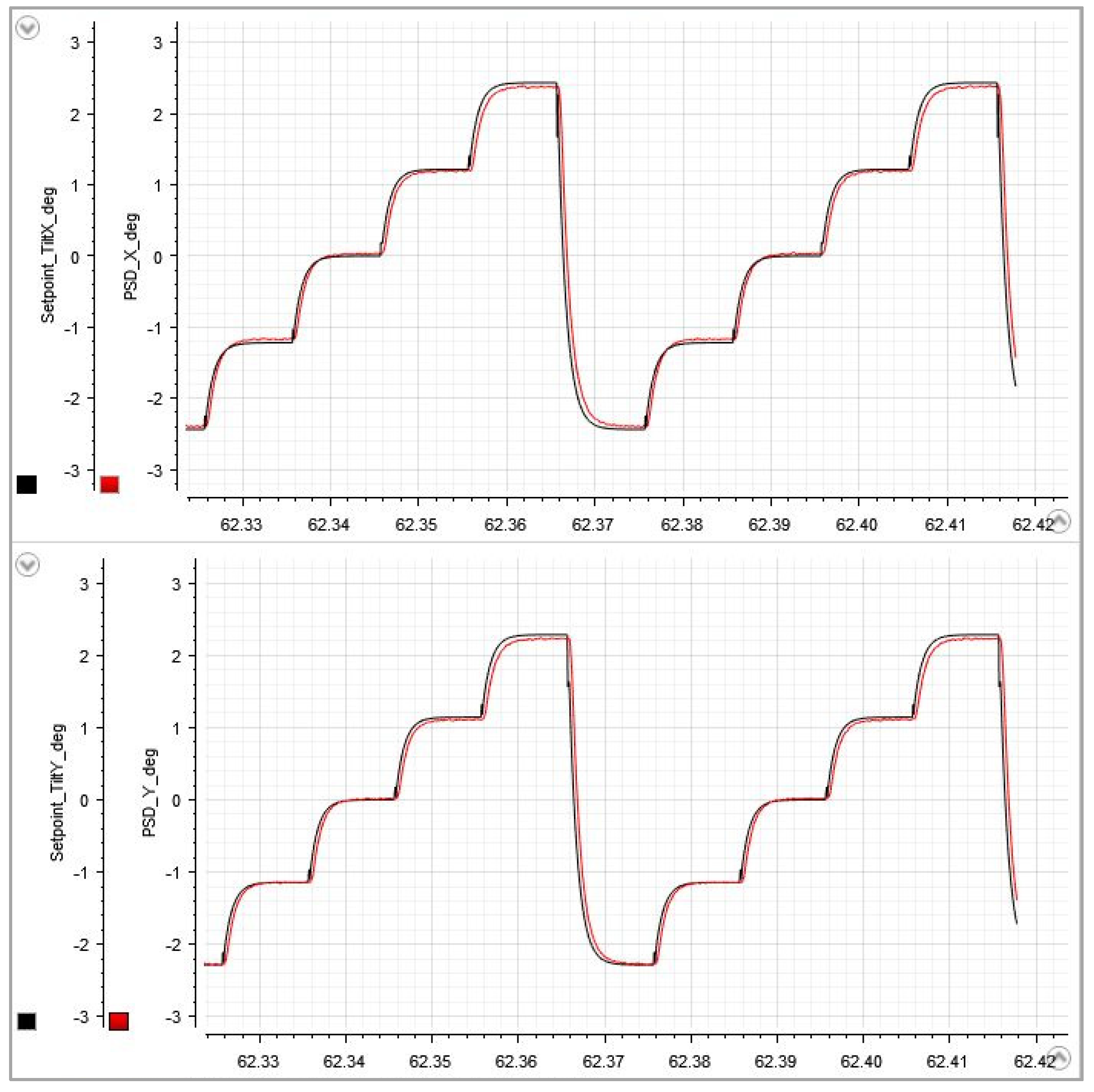
In an additional test pattern, the full test voltage range was divided into five equidistant steps and the switching intervals were reduced to 10 ms. This stair pattern is continuously repeated to check whether a faster repetitive pattern would produce resonant oscillations. It is very useful for fine-tuning the filter characteristics, e.g., by varying the “desired damping” parameter to prioritize either shorter switching times or lower residual oscillations (Figure 6 and Figure 7).
4. Discussion
We presented the calculation and real-time implementation of a simple filter algorithm for underdamped second-order systems and its application to the open-loop control of a gimbal-less, biaxial, quasistatic MEMS micro mirror with piezoelectric AlScN actuators. Owing to the inherently linear piezoelectric material properties of the sputtered AlScN, the MEMS structure follows the assumed mass-spring-damper model sufficiently well to obtain good results with this algorithm in a wide range of applications. We demonstrated how tuning the “desired damping” allows to trade-off between precision and speed in a step-and-settle application. However, the linear filtering approach remains limited in terms of robustness and speed:
Obviously, an open-loop control cannot be robust against external disturbance. With our new piezoelectric sensor structures, we target implementing a closed-loop system capable of compensating external shock events and vibration. However, some electronic signal conditioning will be necessary to capture the piezoelectric charge transfer. This will be developed in a next step.
When it comes to faster positioning sequences, a significantly more complex approach may be followed, e.g., using model-based prediction algorithms. Given the presence of modal coupling between structure elements, a more precise model of the mechanical behavior would be beneficial. Predictive algorithms involve many matrix multiplications that will require a programmable logic or digital signal processor implementation in fast scanning systems.
6. Patents
The sensor structures and arrangement shown in Figure 1 are subject to a patent application process; the first publication date being in October 2023 (DE 10 2022 203 334 A1, WO 2023/194385 A1).
Author Contributions
Formal analysis, Norman Laske; Funding acquisition, Shanshan Gu-Stoppel; Investigation, Norman Laske and Paul Raschdorf; Methodology, Norman Laske; Project administration, Paul Raschdorf, Erdem Yarar and Shanshan Gu-Stoppel; Resources, Paul Raschdorf and Erdem Yarar; Supervision, Shanshan Gu-Stoppel; Writing—original draft, Norman Laske and Erdem Yarar; Writing—review & editing, Paul Raschdorf and Shanshan Gu-Stoppel. All authors have read and agreed to the published version of the manuscript.
Funding
This research was internally funded by the Fraunhofer Gesellschaft zur Förderung der Angewandten Forschung e.V. in the following projects: “MELINDA - Compressed Sensing unterstütztes LiDAR mit kohärenter Detektion bei augensicheren Wellenlängen für autonomes Fahren“ (3/2020 - 5/2023), and “NeurOSmart - Analogous Neuromorphic Accelerators to Enable Efficient and Secure Smart Sensors” (1/2022 – 12/2025).
Acknowledgments
We greatly acknowledge the scientific and technical contributions of our teams in the cleanroom and backend labs. And we thank Gunnar Wille for tirelessly moving our wafers forward and always sharing his competent technical observations and advice.
Trademarks
The terms MATLAB, SIMULINK, MATLAB Coder and SIMULINK Coder are trademarks of The Mathworks, Inc. The terms MicroLabBox, ControlDesk and dSpace are trademarks of dSpace Systems GmbH.
Conflicts of Interest
The authors declare no conflicts of interest.
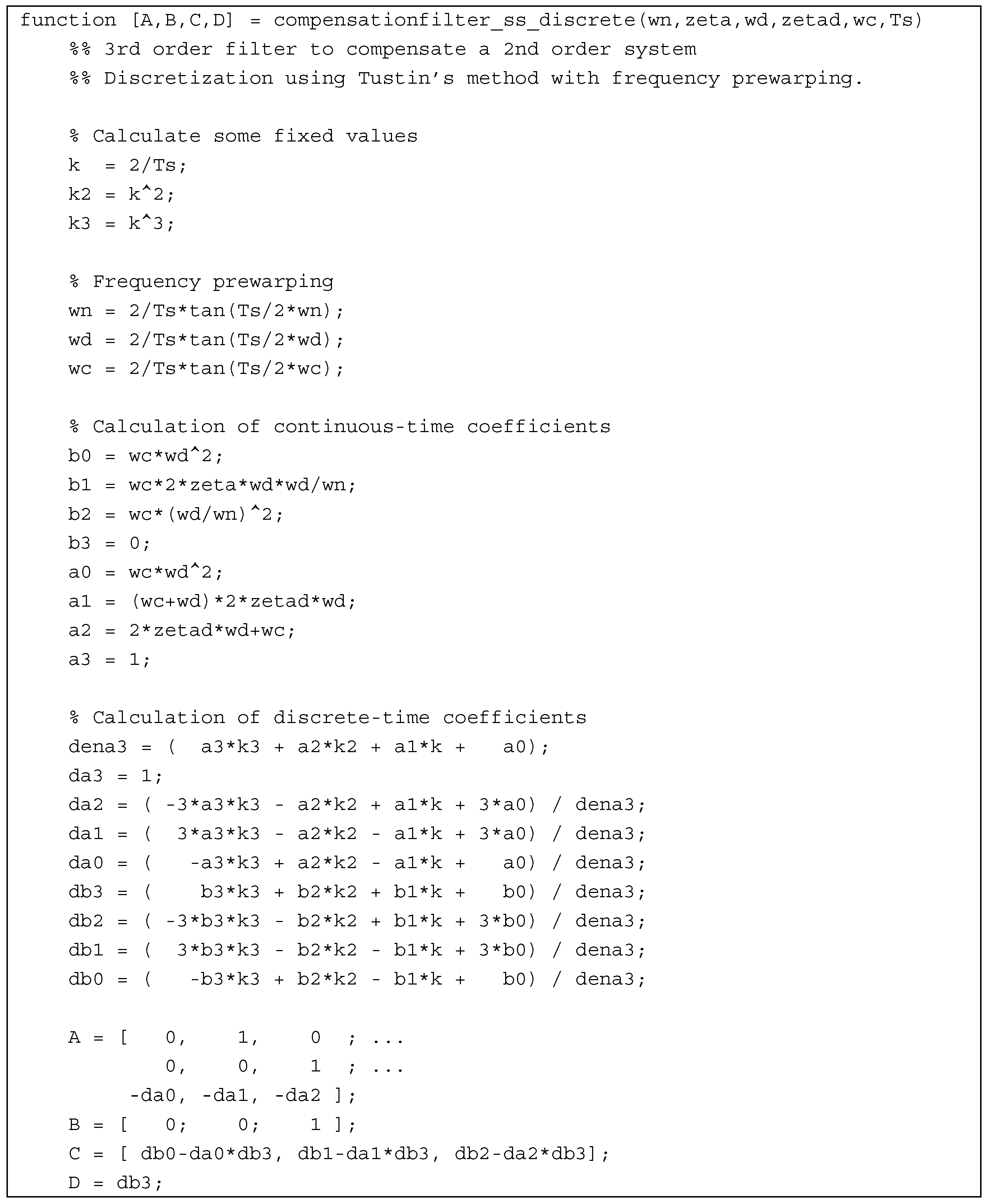
Appendix A
The MATLAB code below implements the filter algorithm explained in Section 2.4. It was used in the SIMULINK model as a user function block, therefore the function end statement is omitted. Some trivial definitions were left in the code for completeness of the mathematical concept.
References
- S. Gu-Stoppel, F. Senger, L. Wen, E. Yarar, G. Wille and J. Albers, “A design and manufacturing platform for AlScN based highly linear quasi-static MEMS mirrors with large optical apertures,” in MOEMS and Miniaturized Systems XX Vol. 11697, 2021.
- S. Gu-Stoppel, T. Lisec, M. Claus, N. Funck, S. Fichtner, S. Schröder, B. Wagner und F. Lofink, „A triple-wafer-bonded AlScN driven quasi-static MEMS mirror with high linearity and large tilt angles,“ in Conference MOEMS and Miniaturized Systems, San Francisco, CA, 2020.
- S. Cwalina, N. Laske, S. Gu-Stoppel, C. Kottke, V. Jungnickel and R. Freund, “Coherent LiDAR with 2D quasi-static MEMS mirror scanning,” in MOEMS and Miniaturized Systems XXII Vol. 12434, 2023.
- S. Cwalina, A. N. Ramesh, N. Laske, M. González-Huici, P. Runge, V. Jungnickel und R. Freund, „Resolution and Speed Trade-offs in FMCW LiDAR with MEMS,“ in European Conference on Optical Communication (ECOC), Frankfurt/Main, 2024 (not yet published).
- L. Stocco, „Optimal 2nd Order LTI System Identification,“ in IEEE/ASME International Conference on Advanced Intelligent Mechatronics (AIM), Seattle, WA, USA, 2023.
- B. Friedland, Control System Design: An Introduction to State-Space Methods, New York, USA: McGraw-Hill (2005 Reprint by Dover Publications, Inc.), 1986.
Figure 1.
(a) The new design features piezoelectric sensor ribbons on each actuator and a few mechanical changes to reduce structural stiffness. (b) With the mirror plate mounted above the actuators, a high leverage translates small actuator displacement into large tilt angles (FEM simulation). (c) Overview with actuator names, and (d) zoom on functional details of the mirror suspension.
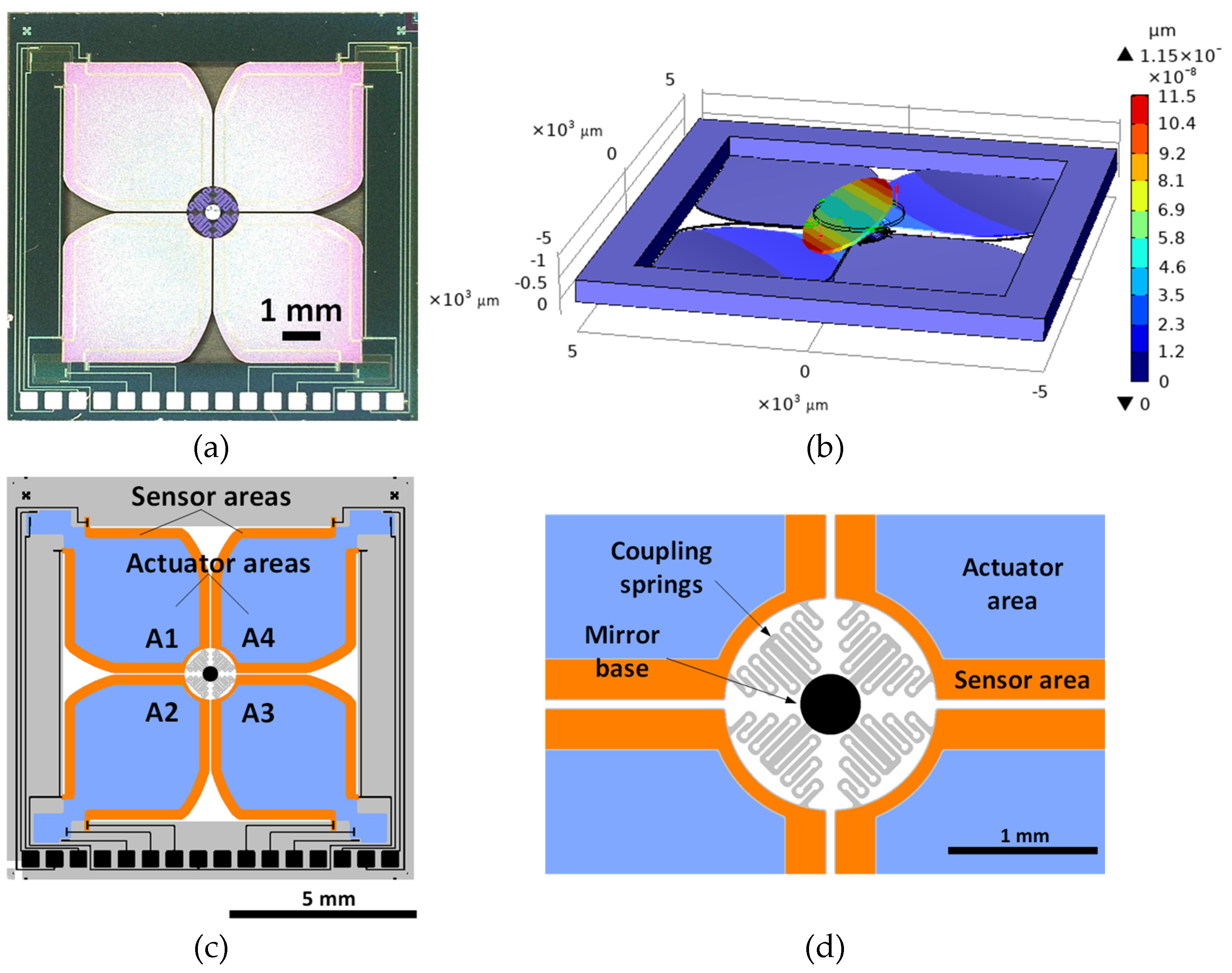
Figure 2.
Bode plots of the amplitude (top) and phase angle (bottom, phase is wrapped to +/-180°) of the mirror’s response, frequency sweep from 2 kHz to 800 Hz. (a) Driving the X-axis only leads to a major resonance peak at 1490 Hz, with some excitation of the Y-axis. (b) Driving the Y-axis shows the resonance at 1520 Hz and a cross-coupling comparable to (a).
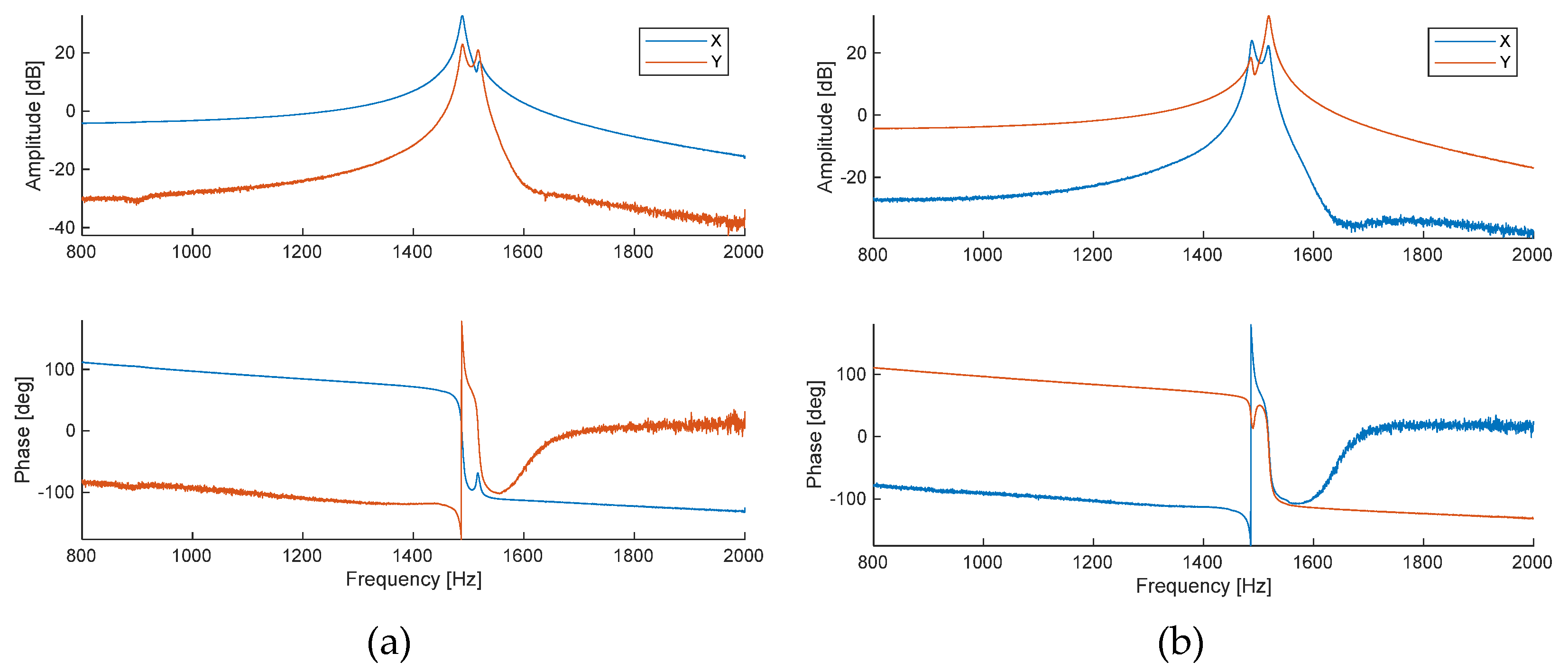
Figure 3.
Linear variation of the actuator voltage from -50 V to +50 V on the X- (top) and Y-axis (bottom). Left half: Time plots (seconds). Right half: Linearity error relative to a +/-20 V reference range.
Figure 3.
Linear variation of the actuator voltage from -50 V to +50 V on the X- (top) and Y-axis (bottom). Left half: Time plots (seconds). Right half: Linearity error relative to a +/-20 V reference range.
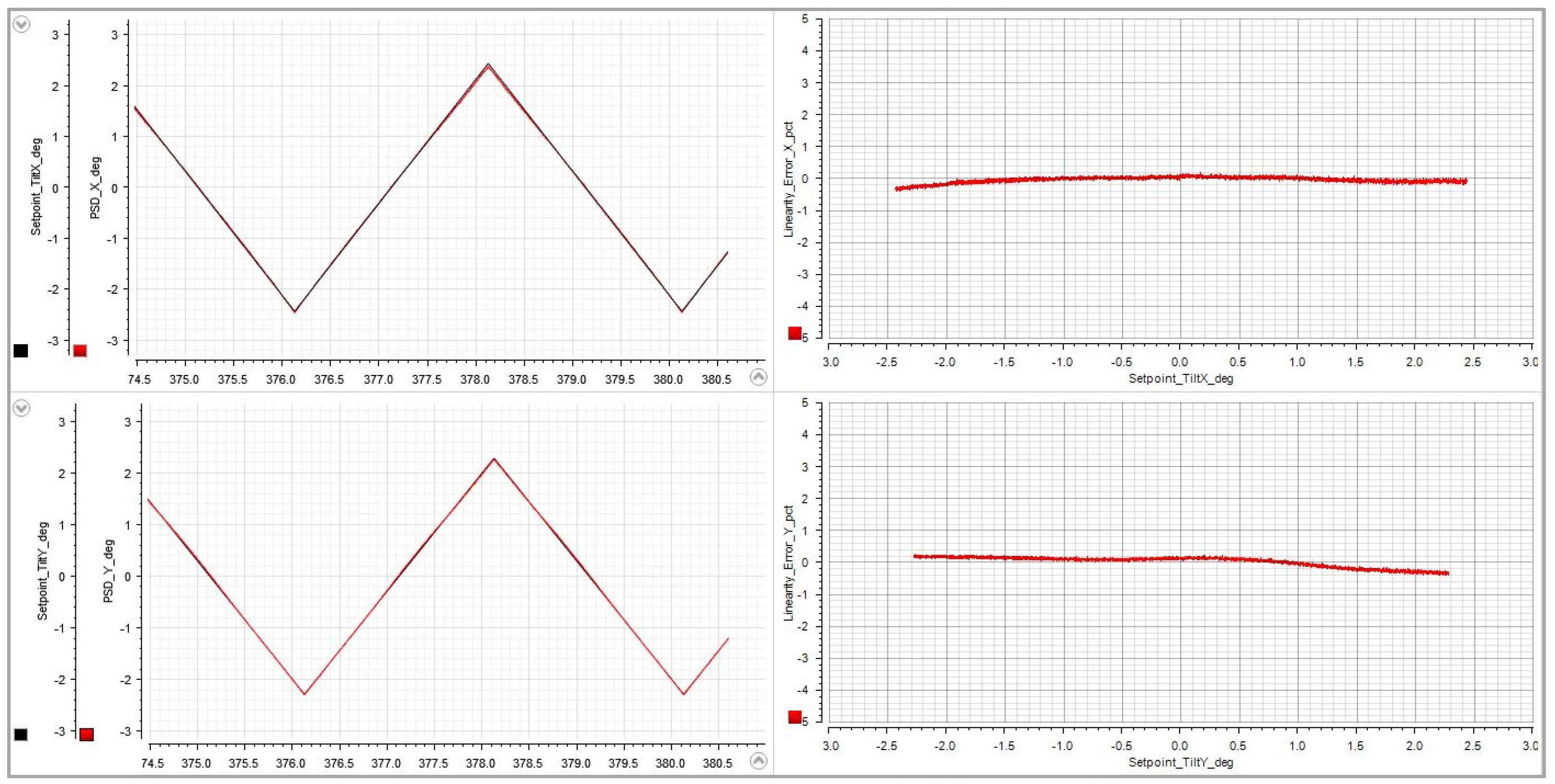
Figure 4.
Step responses without filtering; unidirectional X (top) and Y (bottom) actuation with 50 V are performed simultaneously. X- and Y-axis oscillate at approx. 1580 Hz and 1530 Hz, respectively. Black curves: Control signal. Red curves: Measured optical tilt angle.
Figure 4.
Step responses without filtering; unidirectional X (top) and Y (bottom) actuation with 50 V are performed simultaneously. X- and Y-axis oscillate at approx. 1580 Hz and 1530 Hz, respectively. Black curves: Control signal. Red curves: Measured optical tilt angle.
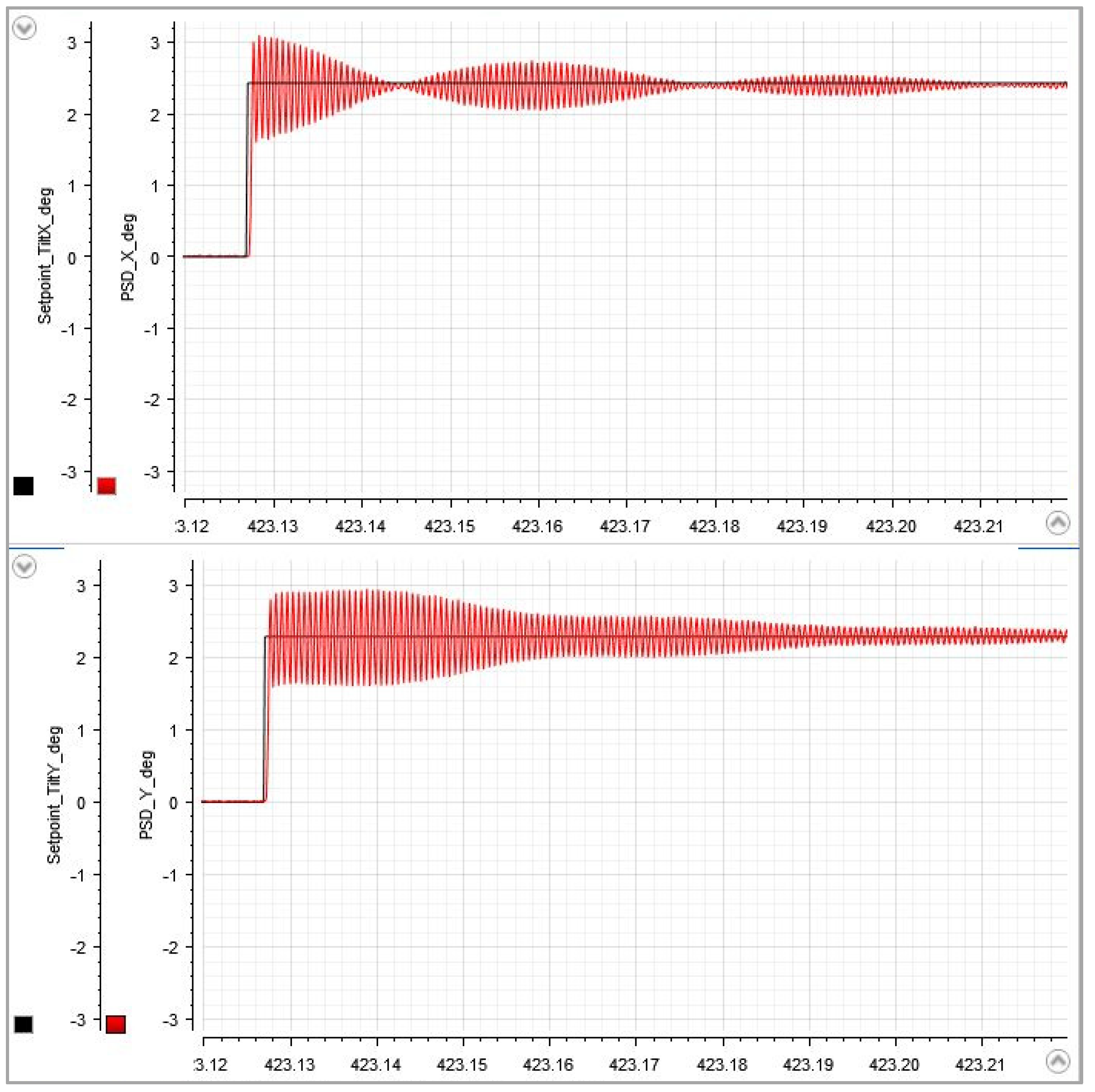
Figure 5.
Step response with activated filter algorithm. The control signals (black) show a characteristic first excitation peak, then smoothly approach the target values. The mirror response (red) absorbs the initial peak and reaches the target deflection angle after approx. 1.5 ms.
Figure 5.
Step response with activated filter algorithm. The control signals (black) show a characteristic first excitation peak, then smoothly approach the target values. The mirror response (red) absorbs the initial peak and reaches the target deflection angle after approx. 1.5 ms.
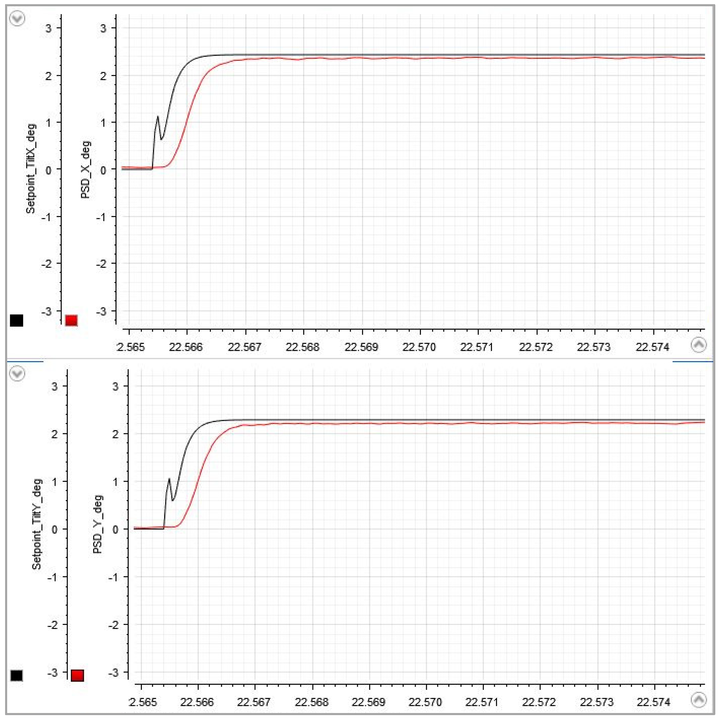
Figure 6.
A periodic stair pattern with a duration of 10 ms for each step. Using a “desired damping” , slight oscillations permanently remain.
Figure 6.
A periodic stair pattern with a duration of 10 ms for each step. Using a “desired damping” , slight oscillations permanently remain.
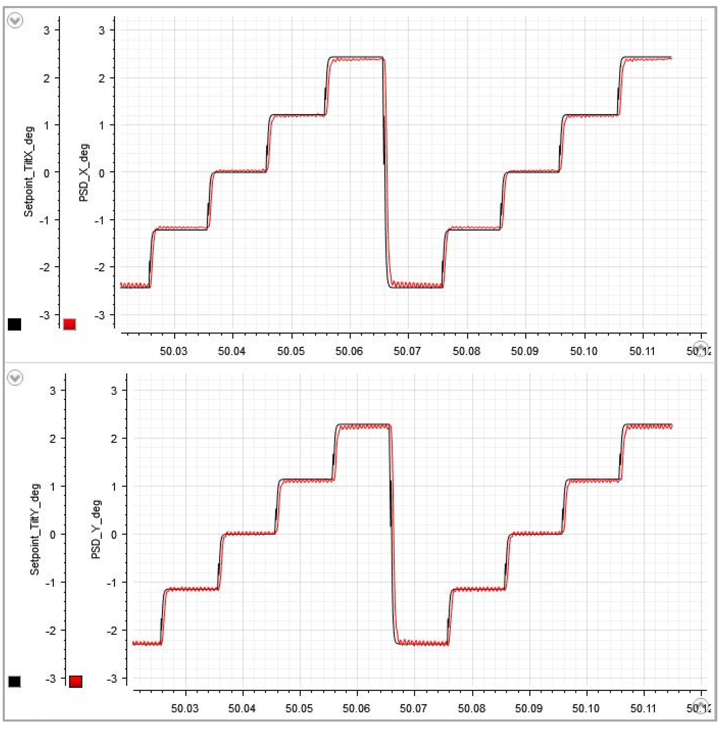
Figure 7.
Changing the “desired damping” to reduces the excitation of undesired oscillations.
Disclaimer/Publisher’s Note: The statements, opinions and data contained in all publications are solely those of the individual author(s) and contributor(s) and not of MDPI and/or the editor(s). MDPI and/or the editor(s) disclaim responsibility for any injury to people or property resulting from any ideas, methods, instructions or products referred to in the content. |
© 2024 by the authors. Licensee MDPI, Basel, Switzerland. This article is an open access article distributed under the terms and conditions of the Creative Commons Attribution (CC BY) license (http://creativecommons.org/licenses/by/4.0/).
Copyright: This open access article is published under a Creative Commons CC BY 4.0 license, which permit the free download, distribution, and reuse, provided that the author and preprint are cited in any reuse.


