Preprint
Article

This version is not peer-reviewed.

Simplified Machine Learning Model as an Intelligent Support for Safe Urban Cycling

A peer-reviewed article of this preprint also exists.

Submitted:

19 December 2024

Posted:

20 December 2024

You are already at the latest version

Abstract

Urban cycling is a sustainable mode of transportation in large cities, and it offers many advantages. It is an eco-friendly means of transport that is accessible to the population and easy to use. Additionally, it is more economical than other means of transportation. Urban cycling is beneficial for physical health and mental well-being. Achieving sustainable mobility and the evolution towards smart cities demands a comprehensive analysis of all the essential aspects that enable their inclusion. Road safety is particularly important, which must be prioritized to ensure safe transportation and reduce the incidence of road accidents. In order to help reduce the number of accidents that urban cyclists are involved in, this work proposes an alternative solution in the form of an intelligent computational assistant that utilizes Simplified Machine Learning (SML) to detect potential risks of unexpected collisions. This technological approach serves as a helpful alternative to the current problem. Through our methodology, we were able to identify the problem involved in the research, design and development of the solution proposal, collect and analyze data, and obtain preliminary results. These results experimentally demonstrate how the proposed model outperforms most state-of-the-art models that use a metric learning layer for small image sets.

Keywords: 
;  ;  ;  ;  

1. Introduction

1.1. Urban Mobility

There is no doubt that population growth is consistent and in Mexico during the last 25 to 30 years, this growth combined with very poor urban planning has caused a problem of vehicle congestion in the nation’s large cities. This situation causes the daily transfer from one point to another and on the outskirts of these large urban cities to take between one and three hours on an average trip, when these trips could normally be made with a duration of between thirty minutes and one hour.
Faced with these circumstances, sustainable mobility became a highly relevant issue for planning urban mobility systems, since it is a model that promotes the use of different means of transport that are friendly to the environment, inclusive and accessible [1]. In this research we are mainly considering three means of mobility that, due to their nature and hierarchy in mobility [2], are considered sustainable: walking, urban cycling and public transport, including this last hierarchy are considered common public transport in Mexico such as the metro, metrobus, light rail, commuter train, trolleybus and cable car. There are multiple benefits that this type of mobility contributes to the environment by not having large amounts of gas emissions, by not having energy waste and even contributing to reducing the carbon dioxide footprint in the atmosphere. With respect to social benefits, since these are collective and individual means of transportation, they significantly promote inclusion and are viable options for making long-distance journeys at a reduced cost.
Within these three means of mobility mentioned above, it is worth highlighting urban cycling, since it is a transportation choice that lightens the load on vehicles in road congestion. It is an ecological option because it promotes the significant reduction of harmful gases such as CO2, it is an accessible means of transportation, easy to use and that, at the same time, contributes to improving both emotional and physical health. However, this alternative requires more attention from the authorities in charge of planning mobility in large cities, since the exclusive lanes are insufficient, the public access systems are limited and high cost for a sector of the population there are not enough spaces to park bicycles or store them, there is also an inequality of spaces to travel and urban cyclists are not given priority in terms of road safety.

1.2. Road Safety for Cyclists

Pedestrians and cyclists head the mobility hierarchy (see Figure 1), which classifies modes of transportation according to the vulnerability they present, as well as both negative and positive peculiarities that they cause as a means of transportation. It is worth mentioning that the negative peculiarities include the possible risks that a certain modality represents for users in other hierarchies.
To promote the use of bicycles, it is necessary to guarantee safety conditions through a focus on preventing road events that cause deaths and injuries. According to the philosophy of the Vision Zero road safety concept [3], which is based on the simple fact that we are all human beings and therefore make mistakes. This is why there is a need to generate systems that support the cyclist during their road trajectory, thereby reducing the possibility that these errors end in injuries and deaths. Institutions such as the World Health Organization (WHO) point out that in the event of a transport accident, the population of cyclists and pedestrians is more vulnerable and their safety is strategic in a global culture that needs to intensify sustainable travel [4].
In Mexico as in other countries we face a great public health challenge as a result of injuries generated by poor road safety. Statistically, it has been reported that traffic injuries are the leading cause of death among children between the ages of 4 and 14 years. Among the highest percentage of deaths are young people between 15 and 30 years old (32.2%), followed by the group between 30 and 44 years old (25.5%) [5], which has a strong impact on the economy and emotional stability of families, as well as society as a whole.

1.3. Intelligent Urban Cycling

Although it is true that the bicycle is in the subconscious of citizens as a pleasant element, associated with a livable city, a majority of citizens would use it when traveling if there were a safe and coherent infrastructure and pleasant environments. In this sense, technology can currently be used as a cyclist’s assistant, which will allow them to travel in a safer way during the trip.
Currently, the aim is to effectively incorporate urban cycling into the transportation networks within the so-called smart cities and promote more modern, clean and safe modes of transportation. This requires establishing an individual mobility model that, through the collection and analysis of various types of data, generate as a result the information that integrates smart mobility [6,7,8].
Correspondingly, the organization of this paper is arranged based on the following sequence:
  • Section 2 is prepared to outline the intuitive information presented by the problem and the main research method adopted to identify the dominant characteristics and advantages of Simplified Machine Learning in achieving unexpected collision risk identification tasks crucial for training and testing procedures for maximize the effectiveness of model classification.
  • Section 3 it is structured to generally explain the methodology used, the essential description of the proposed solution that includes the architecture of the proposed cognitive model as well as its main parts.
  • Section 4 describes the experimental stage used to observe the performance of the model with different datasets and provides comparative tables and graphs that illustrate its performance when using different feature extractors as well as in each of the sample ranges that were used (One-Shot and Five-Shot ).
  • Section 5 provides discussion of notable results related to the evaluation of the proposed model, its generalization capacity and its comparison against other state-of-the-art methods, as well as other particular aspects of its operation and performance.
  • Section 6 expresses the main research conclusions.
Totally, the paper’s contribution is reflected in the following points:
  • Reduce time, effort and costs related to the number of examples or training samples used in conventional Deep Learning (DL) and Machine Learning (ML) models.,
  • This proposal, based on cutting-edge technology, is presented as a novel support option for cyclists, allowing them to travel more safely during trips within urban areas.,
  • Contribution to the area of machine learning with a model that proposes using fewer examples or samples of information for training and being able to resemble the natural learning of human beings.

2. Simplified Machine Learning

2.1. The Challenge of Machine Learning

Increasing safety in urban cycling and its incorporation as a smarter and safer means of transportation towards future smart cities suggests a technologically supported solution to assist the urban cyclist. Intuitively, the problem shows that there is information available and other information that is not. The Table 1 summarizes these two aspects to consider to model a possible solution.
Also intuitively, Figure 2 presents in a general way, the characteristics that a suggested machine learning model should have to be applied to the problem of this research.
The information and intuitive characteristics of the problem to be solved suggest that the proposed solution can be oriented towards the area of artificial intelligence and specifically within the field of machine learning, because to assist the cyclist in identifying the risk of a collision, it must have an accelerated learning process also using previously learned information. Recently, machine learning has been very successful in various tasks, specifically in image and speech classification, pattern recognition or improved searches for information on the web. However, it is also known that these models usually require a large amount of data and training time to have a reliable learning process.
Therefore, the purpose of this research is that based on the approach and description of the problem, a technological solution is proposed that supports the urban cyclist in reducing the risk of collision by focusing on automatic detection within a dynamic environment, so the Research question is defined as follows: Can a machine learning model be used, based on some examples, to learn the concept of unexpected collision risk and detect it in real time?

2.2. Related Work

Reviewing possible technological proposals for solutions to this problem, there are preventive approaches that rely on unsupervised machine learning to explore the circumstances associated with urban cycling safety, such as those exposed by Zhao, H. et al [9], in where large amounts of publicly available data, such as satellite images, neighborhood and city maps, are used to collect information from the environment of cyclist accidents and use machine learning methods, such as Generative Adversarial Networks (GAN) to learn from these data sets and explore the factors associated with cyclist crashes. In this same sense, it is known that work has been carried out in this regard in Spain, such as the one presented by Galán R. et al [10], where the variables that are causes of accidents in bicycle users are studied, with the aim of reducing the number of accidents and thus increase the number of people who use it as a means of transportation with greater safety.
However, in the time in which this research has been carried out, no evidence has been found that a technological proposal that involves a means of transport such as the bicycle and supports the reduction of accidents in this sense has been contemplated. Nor has specific evidence been found of a geospatial analysis of accidents in urban cycling to be able to make a comparison of methodology and results.
It is known that recently machine learning has been very successful in various tasks, such as pattern classification and searching for massive information on the web, as well as image and speech recognition. However, these machine learning models often require, as training input, a large amount of example data to learn. Likewise, the technology known as Deep Learning (DL) [11,12] is booming and has been playing an important role in the advancement of machine learning. However, it also requires large amounts of data.
In addition to this, the large size of the data tends to lead to slow learning, this is mainly due to the parametric aspect of the deep learning algorithm, in which, due to the operating characteristics, the training examples must be learned in parts and gradually. Now, it has been mentioned that one of the characteristics of the Simplified Machine Learning model is that it must be able to learn from very few examples, therefore deep learning would not apply for this purpose. On the other hand, the model should be more similar to the way humans learn, that is, generalize knowledge from a few examples.

2.3. Contrastive Learning

Intuitively we can say that contrastive learning mimics the way humans learn about the world around them. According to many specialists, children learn new concepts more easily, for example by looking at a picture of an owl and trying to find a similar one among a set of images of various animals. In this case, the child has to compare each of the animals by identifying their characteristics, compare them with those of the owl in the original image and then conclude that the image represents a similar animal.
From what was described above, it turns out that it is easier for a person without prior knowledge, like a child, to learn new things by contrasting between similar and different things instead of learning to recognize them one by one. Initially, the child may not be able to identify an owl as such, but after a while the child learns to distinguish common characteristics among owls, such as the shape of their head, their posture, their wings, and the shape of their body.
Within machine learning (ML), contrastive learning is a machine learning paradigm in which unlabeled data is juxtaposed against each other to teach a model which are similar and which are different. That is, as the name suggests, the samples are contrasted against each other and those belonging to the same distribution are pushed towards each other in the same compact Euclidean space. On the contrary, those that belong to different distributions move away from each other [13].
Contrastive learning is a technique that improves the performance of computer vision tasks because it has shown promising results over deep learning, thus gaining importance in the field, by using the principle of contrasting samples with each other to learn the attributes that are common between data classes and the attributes that differentiate one data class from another.
In recent years, there has been a resurgence in the field of contrastive learning which has led to important advances in self-supervised learning [14,15,16,17,18]. The common idea in these works is the following: join an anchor sample and a "positive" sample in the representative space (embedding space) and separate the anchor from many "negative" samples. Since there are no labels available, a positive pair often consists of an increase in sample data, and negative pairs consist of the anchor and samples chosen at random from the small set of images. These concepts are shown by comparing them graphically in Figure 3. Likewise, in [15,16], certain connections are described that exist between contrastive loss and the maximization of similar information when evaluating it between different data samples.

2.4. Approach Overview and Contributions

Contrastive learning as mentioned in Khosla, P. et.al [13] mimics the way humans learn and aims to learn low-dimensional representations of data by contrasting between similar and dissimilar samples. Therefore, humans can learn new things with a small set of examples. When a person is presented with new examples, they are able to understand new concepts quickly and will then recognize variations of those concepts in the future. Just like that, a child can learn to recognize a cat from a single image. However, currently a machine learning system needs many examples to learn the characteristics of a cat and recognize them in the future or in other examples.
We can observe that in standard associative learning, i.e., an animal must repeatedly experience a series of associations between a stimulus and a consequence before it completely learns a particular stimulus. Therefore, learning is inevitably incremental. However, animals sometimes conclude or infer results that they have never even observed before and from which they need to learn quickly to survive. In such cases, animals can learn from a single exposure to the stimulus, in this situation but making an analogy towards machine learning, this is what we have defined as Simplified Machine Learning [19] and that generally It is known in the literature as one-time learning.[20].
Compared to computers, it is a hallmark of human intelligence to be able to learn quickly, whether it is recognizing objects from a few examples or quickly learning new skills after a few minutes of experience. Today it is claimed that artificial intelligence systems should be able to do the same, learn and adapt quickly from a few examples and continue to adapt as these systems are exposed to more and more available data. This type of learning with characteristics of speed and flexibility is a challenge, since the system must integrate its prior knowledge with a small amount of new information, efficiently avoiding overfitting to new data. Likewise, this previous experience and the new data will depend on the task at all times (see Figure 4).
Our solution proposal in terms of being able to support an urban cyclist to ride safely in urban environments is to specify and design the model that can perceive and perform machine learning with few training examples, which assists in risk detection. of collision and thus be able to alert the cyclist of the possible danger.
The main justification behind this Simplified Machine Learning will then be to able to train a cognitive model with one or very few examples, as well as being able to generalize unknown categories without extensive retraining and thus being able to better adapt as a solution to the problem posed in this research.
So far, no concrete evidence of specific work related to the problem has been found, so it is considered that this research is the first attempt to define a machine learning model that allows detecting and evaluating the risk of unexpected collisions in urban cycling.
Some of the work done during our research and presented in this article was inspired by what was developed in [21], which showed how similarity using Euclidean distance ( L 1 ) was superior to similarity using cosine distance presented in [22]. Therefore, it was assumed that adding a combined affinity layer will improve the classification accuracy. With this approach, we proposed to implement this combined affinity layer in our Siamese artificial neural network for One-Shot learning. This is a major contribution to what we have called Simplified Machine Learning, by developing a new type of affinity layer (bi-layer) for deep affinity neural networks, which is the basis of our Siamese Artificial Neural Network.

3. Materials and Methods

Below in this section, a brief general description of the methodology used is presented, the substantial description of the proposed solution that includes the explanation of the architecture of the proposed cognitive model as well as its essential parts such as the Affinity Layers and the Layer Combined Affinity.

3.1. Methodolgy

For the development of this research, the mixed methodology or mixed research route, proposed by Hernández-Sampieri and Mendoza [23] was used as a basis with some variations required for the present work. The main reason for using this mixed methodology is that it does not replace quantitative research or qualitative research, but rather uses the strengths of both types of inquiry, combining them and tries to minimize their potential weaknesses. Likewise, we consider that it harmonizes or is more suited to the problem statement.
Our methodology integrates quantitative and qualitative approaches, and is constituted by the following general stages (see Figure 5):
  • Research problem statement;
  • Design and development of the solution proposal;
  • Data collection and analysis;
  • Preliminary Results.

3.2. Cognitive Model Architecture

The metric learning [24], that is, learning with a distance measure or Similarity learning is a method that performs mapping in the feature space through feature transformation to subsequently form groups within the feature space. Metric learning based methods are widely used to facial recognition and person identification. Metric learning learns the similarity of two images through the distance between them, where similar targets move closer in distance and different targets move further away from each other. Therefore, metric learning requires certain key characteristics of the learning objectives, that is, individualized characteristics of each object.
By distinguishing different objects, the appearance characteristics of similar objects are very similar, these characteristics belong to the common characteristics between almost identical objects. Distinctive characteristics such as shape, color, texture and size are used to distinguish the different characteristics of two or more objects. Metric learning distinguishes different identities by learning key distinguishing features.
The most commonly used methods for measuring efficiency or loss within metric learning include binary cross-entropy loss, contrastive loss, triple loss, and quaternion loss.
As background, contrastive loss was introduced in 2006 by Hadsell, Chopra and LeCun [25] , and is generally described as a learning loss metric function that calculates the Euclidean distance or cosine similarity between pairs of vectors. Assigns a loss value based on a predefined margin threshold. If the distance between two vectors is less than the margin threshold, the loss value is equal to zero. If the distance is greater than the margin threshold, the loss value increases and is greater than zero. Contrast loss plays a crucial role in maintaining the similarity and correlation of latent representations across different information modalities. This ensures that similar cases are represented by similar vectors and different instances are represented by different vectors.
In a simple way, the loss in metric learning can be exemplified as follows: having two input images x 1 and x 2 , extracting their respective characteristic vectors f x 1 , f x 2 , the Euclidean distance can characterize the similarity, that is, the closeness between two objects through the distance in Euclidean space, defined in the Equation 1 (adapted from [25]) as:
D x 1 , x 2 = f x 1 f x 2 2
Formally, a contrastive loss function is used to learn the parameters W of a parameterized function G W , such that matching neighboring objects move together and non-neighbors move away. The prior knowledge will then be used to identify the neighbors in each case for a training data. As exemplified by Hadsell et al. [25] is an energy-based model that given the neighborhood relations, these are used to learn the mapping function. In this context, given a family of functions G (such as a CNN), parameterized by W (weights of a CNN), the objective will then be to find values of W that map a set of high-dimensional input values by means of a comparator, for example the Euclidean distance to perform "semantic similarity" of the entries in the input space, providing a set of neighborhood relations.
Contrastive loss is mainly used to train so-called Siamese neural networks, introduced in the early 1990s by Bromley et al. [26]. The Siamese network is a "connected neural network", and its network structure is shown in Figure 6.
Algorithm 1: Training of generic Siamese neural network.
Require: 
S - Training dataset, f - CNN, z i j - binary label ( z i j 0 , 1 ) , w - Shared weights, η - Learning rate
Ensure: 
L ( x i , x j , z ij )
1:
for S x i , x j , z i j , i , j K do
2:
    h i f ( x i ) Feature vector of x i
3:
    h j f ( x j ) Feature vector of x j
4:
    d h i , h j h i h j 2 Euclidian distance
5:
   Contrastive Loss function L ( x i , x j , z ij ) (Equation 3)
6:
   Total error function to be minimized L ( w ) (Equation 2)
7:
   Optimize and update weights w n + 1 w n η f ( w n )
8:
end for
Here we see that the network has a "connected body" through sharing the set of weights, that is, the weights of the two neural networks are the same. The Siamese network is mainly used to measure the similarity between two inputs, which can be generated from a CNN or an LSTM [27]. For example, when two images are input, the two inputs are fed into two neural networks, these two neural networks map the inputs to the new representation space separately, allowing the input to be represented as a value within the new space. The similarity or dissimilarity between both inputs is evaluated by calculating the loss value itself.
Let’s say that each pair of training images intrinsically has a binary label Y assigned to this pair. If Y = 0 , x 1 and x 2 are considered similar; otherwise if Y = 1 . Then the contrastive loss function in its general form can be defined as:
L ( W ) = i = 1 p L ( W , ( Y , X 1 , X 2 ) i )
L ( W , ( Y , X 1 , X 2 ) i ) = ( 1 Y ) L S ( D i ) + Y L D ( D i )
where X 1 and X 2 are a pair of input vectors shown to the system, in our case, they are the feature vectors of the input images, ( Y , X 1 , X 2 ) i ) is the i t h labeled pair of samples, L S is the partial loss function for a pair of similar points, L D is the partial loss function for a pair of different points and D to shorten the Euclidean distance notation D X 1 , X 2 . Finally P is the number of training pairs. Both the function L S and the function L D must be designed such that by minimizing L with respect to W results in low values of D for similar pairs and high values for D in different pairs.
Specifying then, the exact loss function will be the Equation 4:
L c ( W , ( Y , X 1 , X 2 ) i ) = ( 1 Y ) 1 2 ( D ) 2 + Y 1 2 m a x ( 0 , m D ) 2
where m > 0 is a margin. The margin defines a radius around G W ( X ) , which is a set threshold. It can be known from the contrastive loss that the loss function can be used both to express the coincidence of pairs of samples and to train the model with the extracted features effectively. With all this, through the continuous reduction of the loss value, the distance between pairs of similar samples is continuously reduced, while the distance between pairs of dissimilar samples is continuously increased.
The general description of the architecture of the proposed Siamese cognitive model is presented in Figure 7. We established as a basis for our Siamese network model an approach similar to the one shown in [27], but adjusting the Convolutional Neural Networks (CNNs) to generate 1024 features instead of 4096, they will also share the same parameters since they are copies of the same CNN. The neural network architecture that learns image embeddings and attribute vectors in the same vector space (embedding space) was used in the implementation of the feature extractor, in this way the distances between affinity features can be calculated. The two input images ( x i , x j ) feed the CNNs, where the two fixed-length feature vectors, f ( x i ) and f ( x j ) are obtained. Since both feature extraction networks are the same, f ( x i ) f ( x j ) if the two images are affine and f ( x i ) f ( x j ) otherwise.
As main feature extractors, the standard CNNs in the state of the art (ResNet-18 [28] and EfficientNet-B0 [29]) were used, which helped to accelerate the training time of the proposed model when generating fewer parameters on the network. Subsequently, these results will feed the affinity layers as detailed in the following section.

3.3. Affinity Layer Overview

In the design and specification of the affinity layer, these are calculated using for A 1 the Euclidean distance, shown in Equation 5 and for A 2 the Manhattan distance, as seen in Equation 6, where u and v are the feature vectors. We adapt for the proposed model, a perspective shown in [27,30] to integrate as the layers in an artificial learning neural network. In this way, a one-to-one operation is performed on each element of the feature vectors and to finally generate a new one.
δ e ( u , v ) = i = 1 n u i v i 2
δ m ( u , v ) = i = 1 n u i v i

3.4. Combined Affinity Layer Overview

The basis of our Siamese artificial neural network is the so-called combined affinity layer C that unifies the feature vectors of the Euclidean ( A 1 ) and Manhattan ( A 2 ) layers to form a single one that will evaluate similarity or dissimilarity of the input images.
The combined affinity layer A m a x works as follows, we take the element-wise maxima of the two affinity layers ( A 1 and A 2 ). Assuming that A = ( A i k ) is the affinity layer, for 1 i m and 1 k n , where m is the total number of affinity layers , and n is the size (number of rows) of each affinity layer, then the corresponding maximum of elements in each row of the two layers are taken to form a layer of size n, which is defined by Equation 7.
A m a x ( k ) = max ( A i k ) , 1 i m
In the design and implementation of the combined layers, the 1024 output of the CNNs was conditioned with a ReLU activation function, a kernel regularizer to prevent overfitting, and a bias initializer. The regularizer works with a mean of 0, while the bias initializer had a mean of 0.5 and a standard deviation of 0.01. Having two inputs to compare each of the model’s feature extractors produces a vector of 1024 features. Those outputs then become the inputs for the two separate layers to calculate the corresponding affinities. The layer A 1 (Euclidean distance, L 1 ) and the layer A 2 (Manhattan distance, L 2 ). In each of these affinity layers an output of 1024 features is produced. Subsequently, it is passed through the Maximum Affinity Layer A m a x ( k ) , which finds the maximum number of elements of the two layers and generates a maximum vector of 1024 features. As a last step, a sigmoid activation function is applied on a layer with a filter, which will produce a value between 0 and 1, which establishes the probability of affinity between the input images.

3.5. Dataset Overview

In the area of One-Shot learning, much of the research evaluating models for image categorization commonly uses the MiniImageNet [22] and CIFAR-100 [31] datasets. For this reason, we used both data sets in the experimental phase, which allowed us to compare them with other state-of-the-art methods that have also used them. Furthermore, we also added the CUB-200-2011 (Caltech-UCSD Birds-200-2011) dataset [32] which has recently been the dataset for comparing Few-Shot Learning tasks, as well as being the most used dataset for fine-grained visual categorization tasks. We also incorporated the DroNet dataset [33] to establish a comparison with a proposed autonomous drone driving approach for obstacle avoidance and make our evaluation and comparison more comprehensive.
As a common practice in the area of machine learning, each dataset was divided into three subsets for One-Shot learning: the training set ( T s ), the validation set ( V s ) and the search/query set ( Q s ). T s is a disjoint set of the sets Q s and V s , but V s and Q s belong to the same category or class. Suppose there are a number i of categories in the training set, a number j of categories in the validation set, and a number k of categories in the search set. The set of category labels in T s , V s , and Q s would then be C i ; C j and C k , respectively.
Therefore, the label pairs for the images in the training set would be set by Equation 8.
T s = x i , x j , A x i , x j i , j = 1 . . n
For which ( x i , x j ) are the image pairs in the training set and A ( x i , x j ) will be the affinity score of the image pair. Therefore, if x i and x j are equal, then the score will have a value of 1 and otherwise it will have a value of 0. It is set to n as the number of training samples or examples.
Continuing with the label specification, Equation 9 names the image label pairs in the validation set.
V s = x k , x l , A x k , x l k , l = 1 . . m
For which ( x k , x l ) are the image pairs in the validation set and A ( x k , x l ) is the affinity score of the image pair. Therefore, if x k and x l are equal, then the score will take a value of 1 and otherwise it will have a value of 0. m is the number of samples or examples for validation.
Finally, the images that form the query set are specified in Equation 10:
Q s = x k k = 1 . . n
For which x k are image samples from categories in the validation set. The final objective sought in this learning is to classify samples in the search/query set given some examples in the validation set meeting the following restrictions: C i C j ; T s V s = ; T s Q s = and Q s V s . Therefore, the categories in the training versus validation set are disjoint, but those classes in the validation and query set are intersecting sets.
The segmentation of the data sets used for the experimental phase of this study are briefly presented below:
  • The MiniImageNet dataset as stated in Vinyals et al. [22] contains 100 classes chosen randomly from the original ImageNet dataset and each of those classes is itself composed of 600 images. The data set was divided following what was presented in [30,34,35,36], into 64, 16 and 20 training, validation and test classes, respectively. The main reason for using this data set is due to its complexity and its repeated use to test many other One-Shot learning tasks.
  • The CIFAR-100 dataset as stated in [31] contains 100 classes with 600 images each. The data set was divided as suggested in [22,34,35,37] into 64, 16 and 20 training, validation and test classes, respectively. This division is in line with other research that evaluated one-shot learning models with this dataset.
  • The CUB-200–2011 dataset defined in [32], as previously mentioned, is a fine-grained dataset consisting of 200 classes and 11 , 788 images. A split was applied to the dataset similar to the one proposed in [34] of 100, 50, and 50 classes for training, validation, and testing, respectively, which in turn is in line with the splits also established in [14,21,22,35,37,38,39].
  • The DroNet dataset as described in Loquercio et al. [33], contains 32,000 images distributed in 137 classes for a diverse set of obstacles. The data set was divided into 88, 22 and 27 training, validation and testing classes, using a data set division similar to that proposed in [22,34,35,37].

4. Results

4.1. Experimental Setup

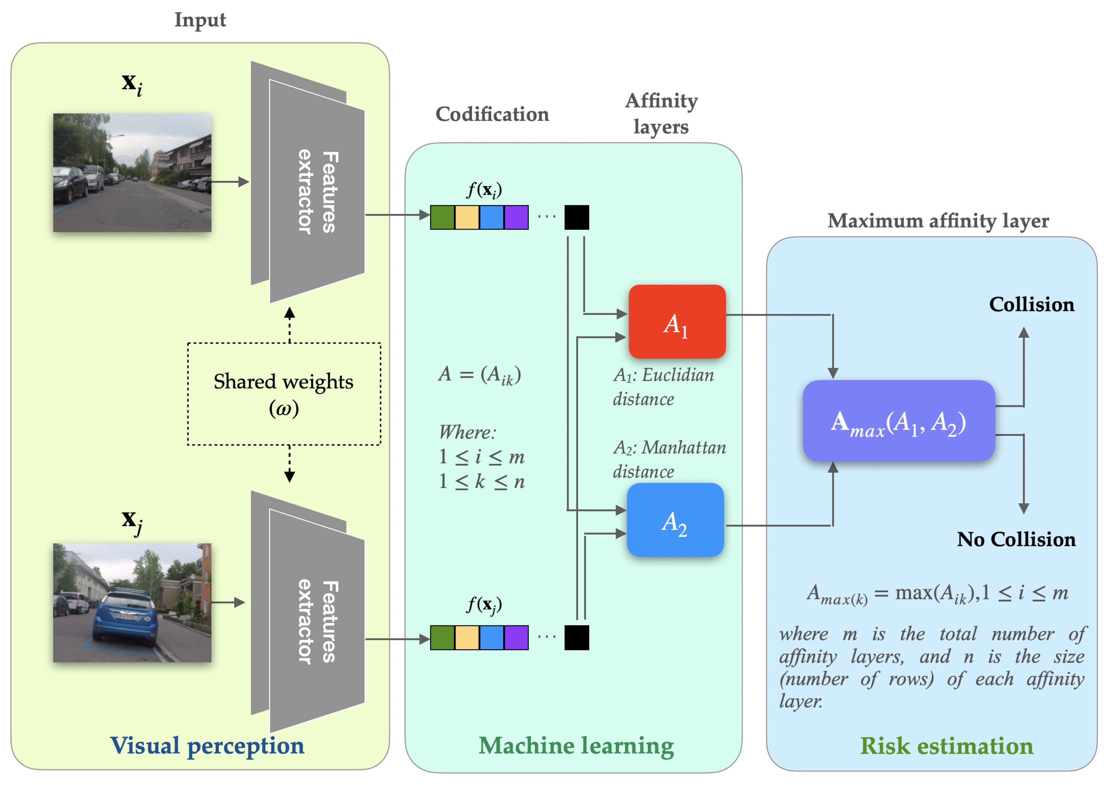
In our experimental phase, two CNN networks were used: EfficientNet-B0 and ResNet-18. These two neural networks were chosen mainly for their characteristics as feature extractors, generalized use in other One-Shot learning models and to be able to compare our results against those in the state of the art. For our model, the ResNet-18 implementation was similar to the one shown in [28], except that the input image size was set to 100 x 100. On the other hand, the EfficientNet-B0 network implementation is similar to the one presented by [29], except also that the input image size was also set to 100 x 100. The outputs are then passed through the proposed combined affinity layer with a sigmoid activation to determine similarity or dissimilarity.
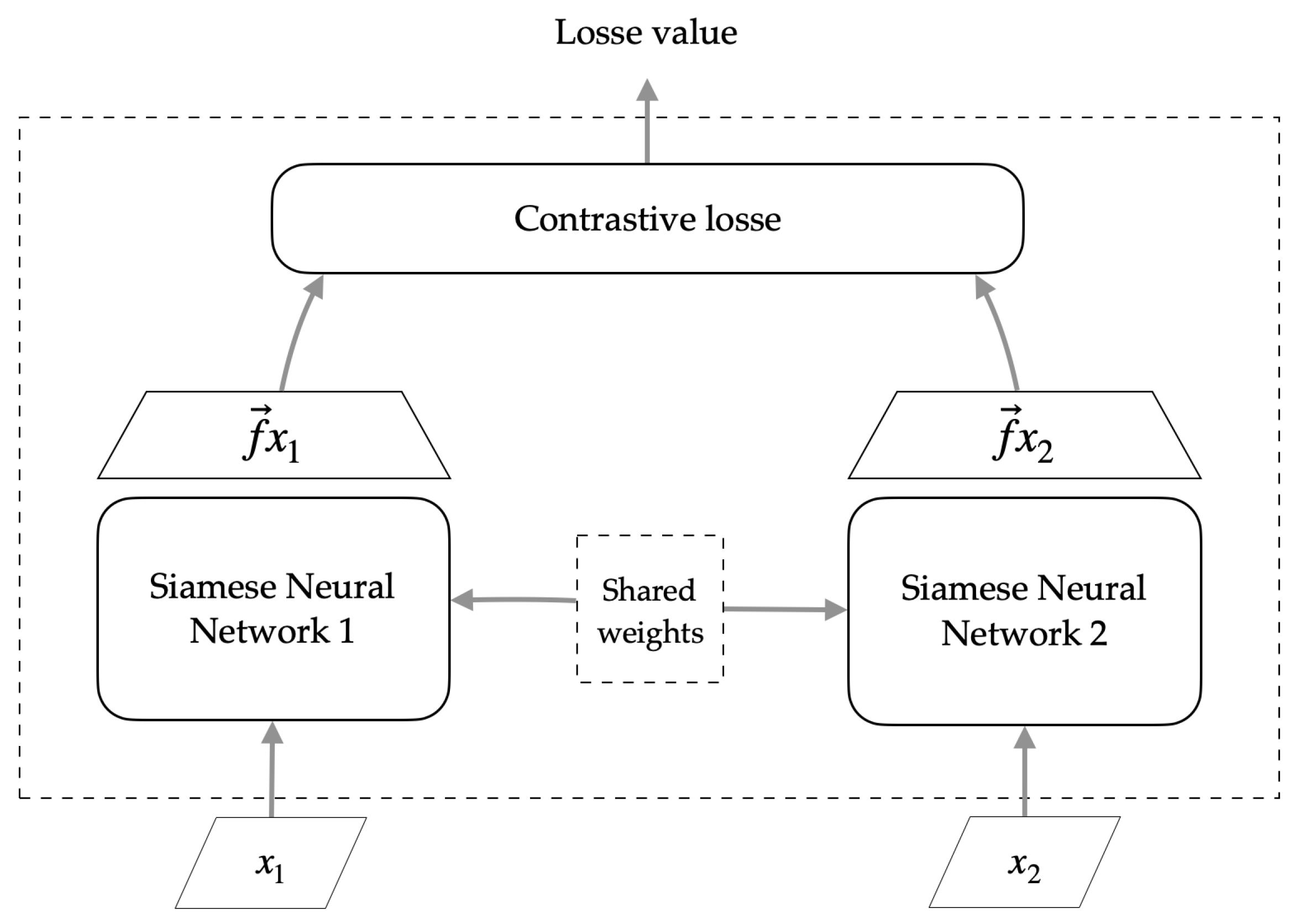
In the experimental design, the number of epochs was established as 200, as well as the size of the processing block was defined as 18. For the training part of the Siamese network, the contrastive loss function (Equation 4) was used as an objective function. Likewise, an Adam Optimiser was also used with an initial learning rate set to 0.0005.
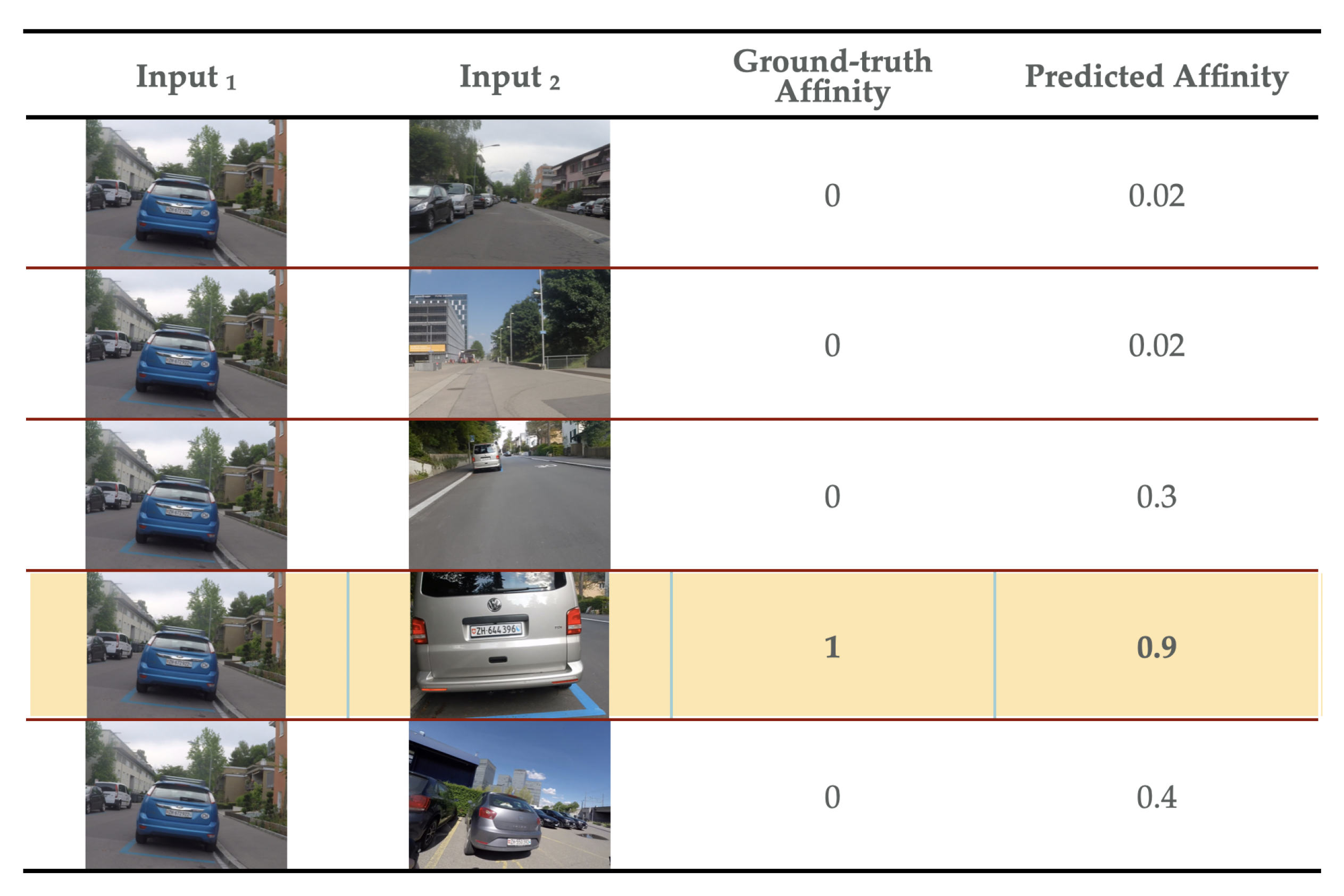
A comparison was made with the current reference models in the literature, which are based on the cosine, Manhattan and Euclidean similarity layers, with the combined affinity layers proposed for the four datasets MiniImageNet, CIFAR-100, CUB-200–2011 and DroNET detailed in previous section. The evaluation was specifically performed on the accuracy of five random example images in 1-Shot mode and five random example images in 5-Shot mode. The above described is exemplified below in Figure 8
The following section presents a comparison of our experimental results in a descriptive and detailed manner, using representative tables and figures.

4.2. Comparison of the Model Against Reference Data

Once the experimental phase has been carried out, the results obtained with each of the data sets used to evaluate the behavior, performance and efficiency of the model are presented below. Likewise, a comparison is made of the model developed in this research against the various models present in the state of the art to also observe its performance and efficiency.
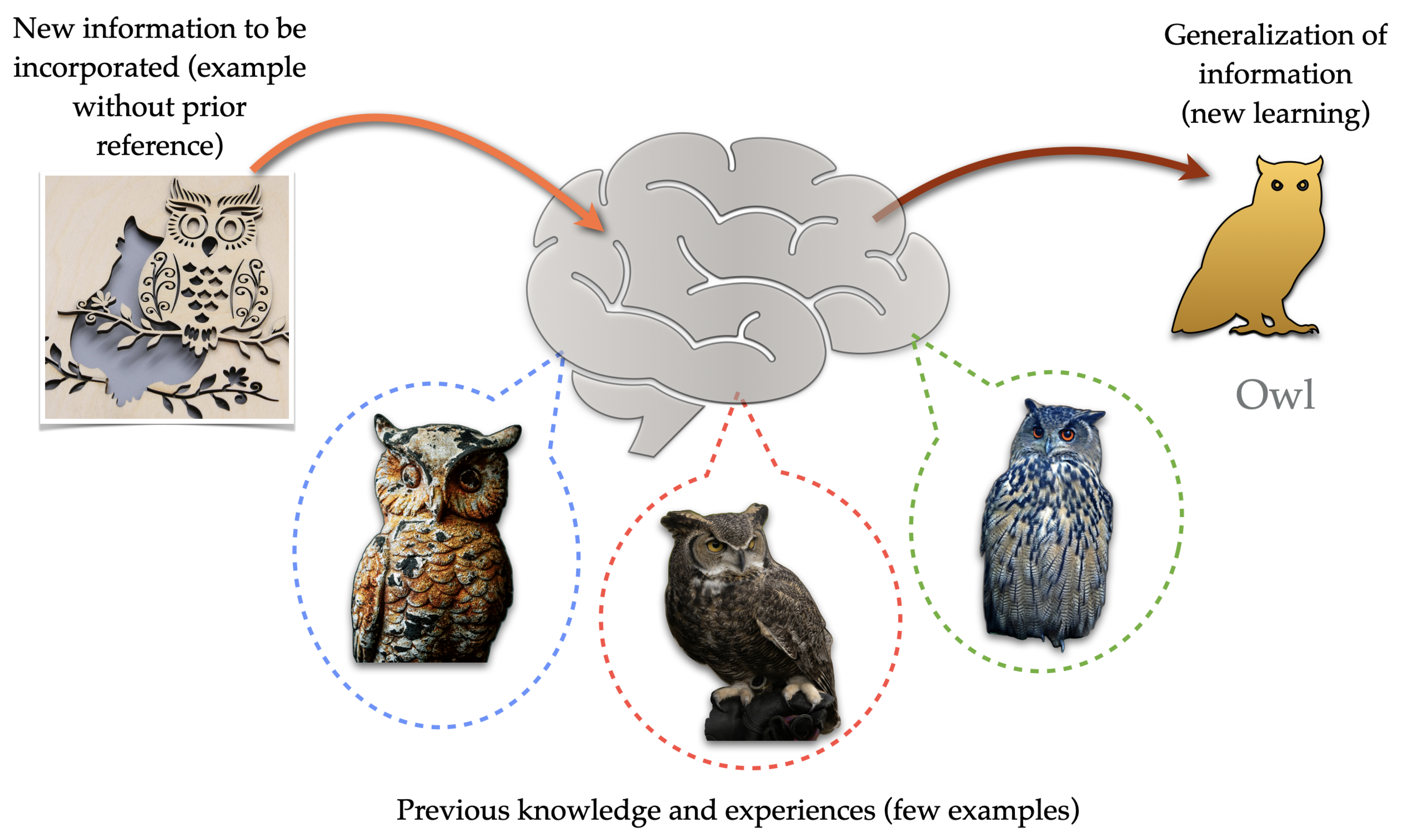
The main objective of the present research focused on developing a biologically inspired computational model, which would allow simplified machine learning using few examples to detect a possible risk of unexpected collision and thereby assist the cyclist in driving within an urban environment. Therefore, the model was specifically evaluated in the accuracy in the identification of perceived information (images) using the single example mode (1-Shot) and for the five-example mode (5-Shot), likewise a comparison with the data sets, using the two feature extractors indicated.
Table 2 and Table 3 shows the average accuracy with 95% confidence when performing image classification using the four data sets, the affinity methods separately, and the proposed SML model ( A m a x layer). Training was performed using the MiniImageNet dataset and the ResNet-18 and EfficientNet-b0 CNNs as feature extractors.
The results show that for all datasets and feature extractor networks our SML model outperformed one-shot mode learning methods (1-shot classification accuracy) using separate similarity layers A 1 (Euclidean), A 2 (Manhattan). Therefore, our SML model using both the ResNet-18 and EfficientNet-B0 feature extractors had the best performance in all cases.
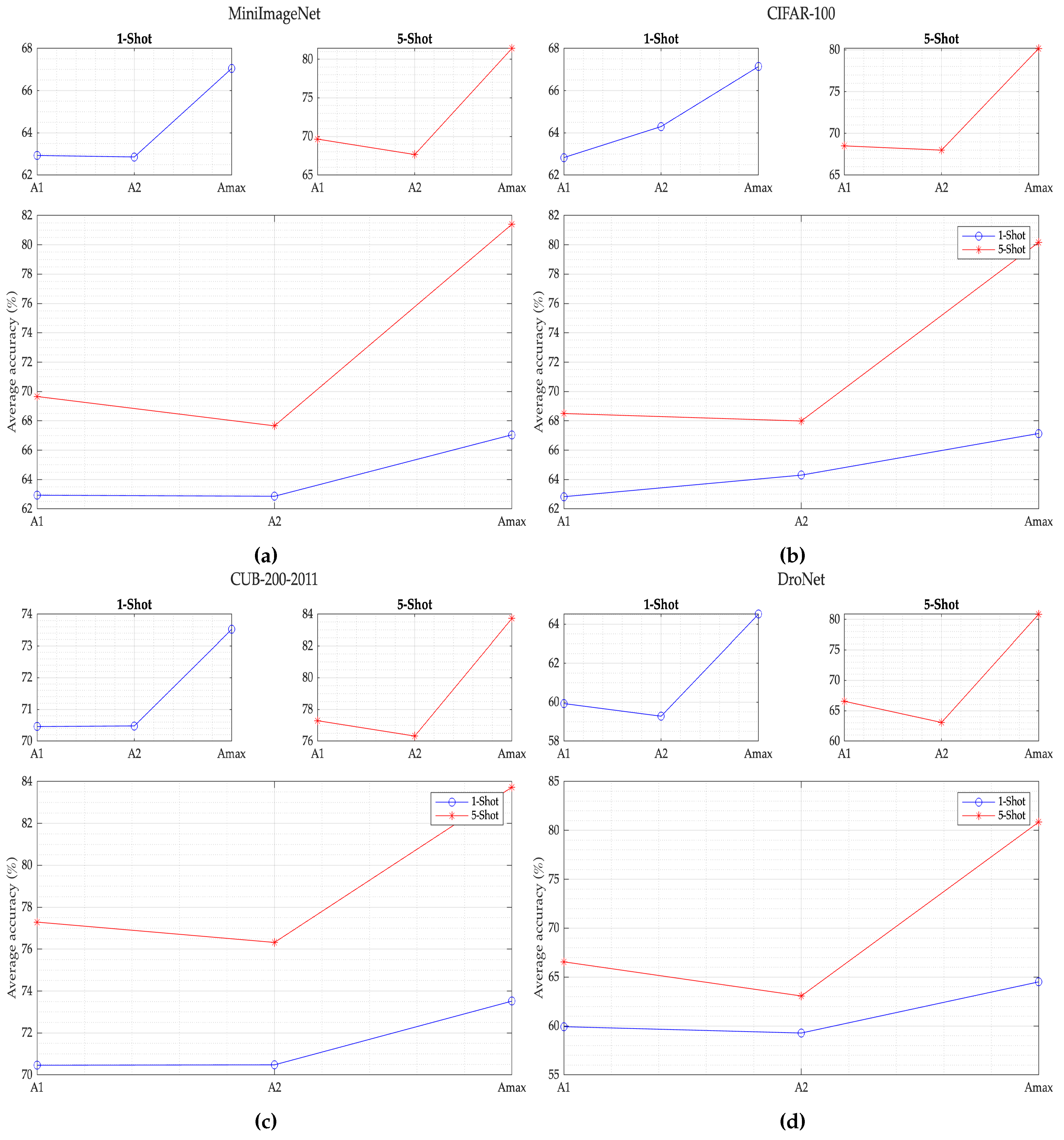
As can be seen in Figure 9, the proposed SML model for the MiniImageNet dataset, with ResNet-18 feature extractor, in 5-Shot mode, performs better by 16.85 % compared to the best result which is similarity layer A1. On the other hand, in the 1-Shot mode, the model performs only 6.55 % better compared to the best result for this mode which is the similarity layer A1.
Next for the CIFAR-100 dataset dataset as shown in Figure 9, the SML model with the same feature extractor ResNet-18, in 5-Shot mode, performs better by 17.04 % compared to the best result which is the similarity layer A1. Likewise, in the 1-Shot mode, the model performs better only by 4.41 % compared to the best result for this mode which is the similarity layer A2.
Continuing with the analysis, as shown in Figure 9, the proposed SML model using CUB-200–2011 dataset, with ResNet-18 feature extractor in 5-Shot mode, performs better by 8.33 % compared to the best result which is similarity layer A1. Now in the 1-Shot mode, the model performs only 4.31 % better compared to the best result for this mode which is the similarity layer A2.
Finally, as seen in Figure 9, for the DroNet dataset the SML model with a similar feature extractor (ResNet-18), in 5-Shot mode, performs better by 21.46 % compared to the best result which is the similarity layer A1, being the best performance within the four datasets used for the 5-Shot mode. Similarly, in the 1-Shot mode, the model performs better by 7.64 % compared to the best result for this mode which is also the similarity layer A1, this being also the best performance within the four datasets used for 1-Shot mode.
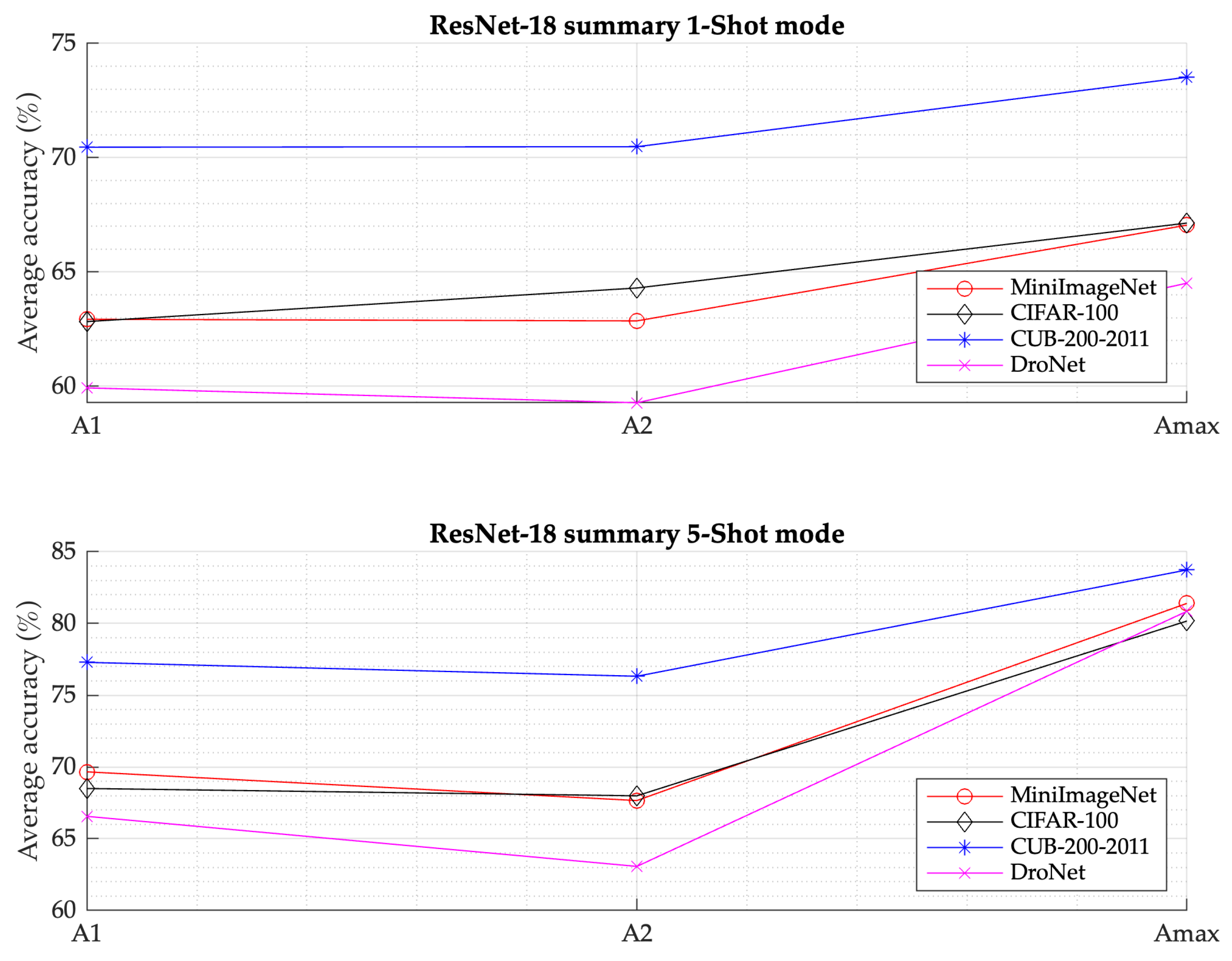
Figure 10 summarizes the previous results comparatively, as well as the behavior of the four datasets using the ResNet-18 convolutional network as a feature extractor, as well as the affinity layers ( A 1 , A 2 and A m a x , used in the comparative.
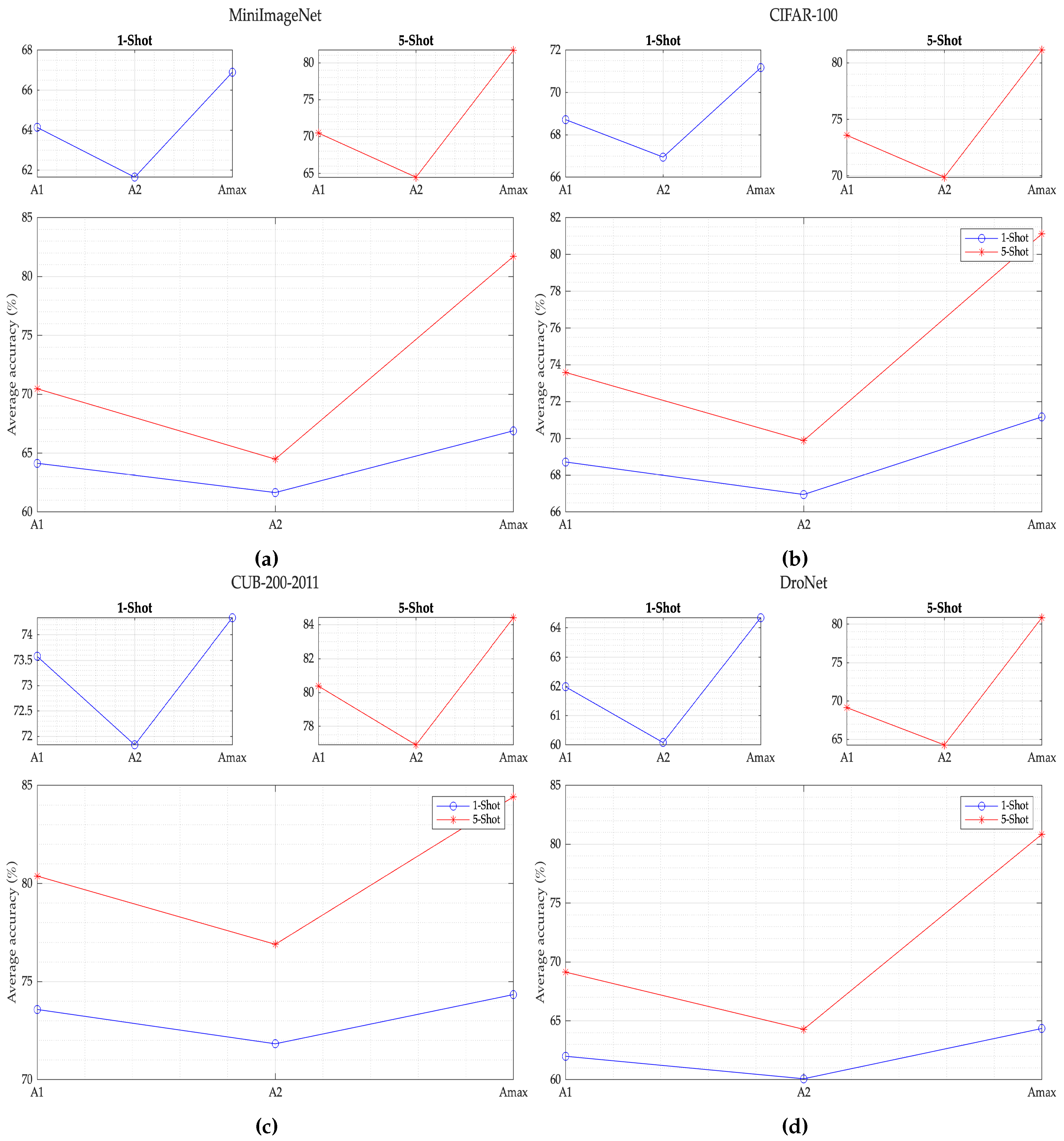
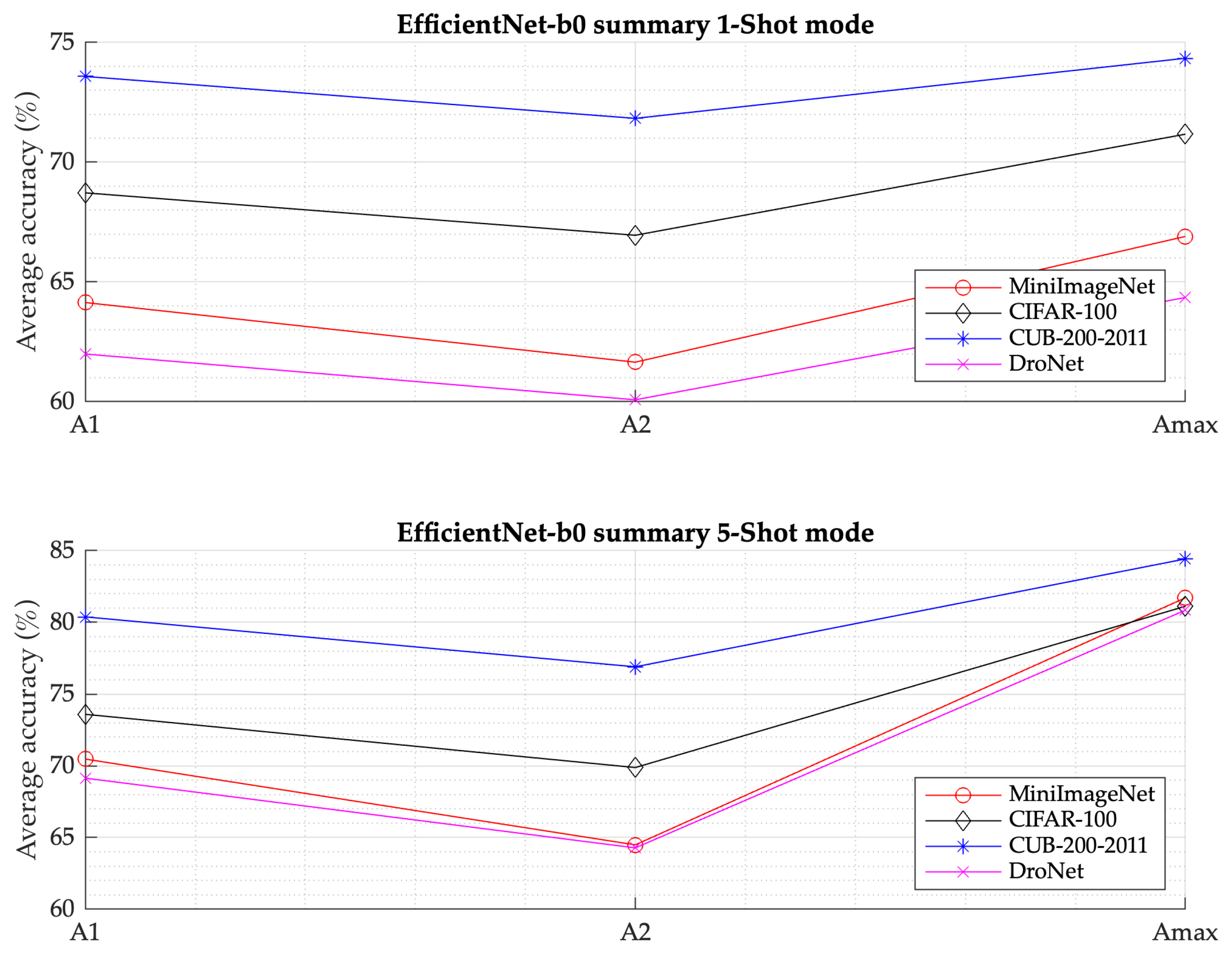
Continuing with the analysis of the results, it can be seen in Figure 11 that the proposed SML model for the MiniImageNet dataset, the SML model with the EfficientNet-b0 as a feature extractor, in 5-Shot mode performs best way with 15.95 % compared to the best result which is the similarity layer A1 . Likewise, in the 1-Shot mode, the model performs better by 4.30 % compared to the best result for this mode, which is the similarity layer A1. It should be noted that this is the best performance among the four data sets used in 1-Shot mode.
Now, for the CIFAR-100 dataset as shown in Figure 11 the SML model with the same EfficientNet-b0 feature extractor, in the 5-Shot mode it performs better by 10.23 % compared to the best result which is the A1 similarity layer. On the other hand, in the 1-Shot mode, the model performs only 3.57 % better compared to the best result for this mode which is the similarity layer A1.
Continuing with the analysis, as shown in Figure 11, the proposed SML model using CUB-200–2011 dataset, with EfficientNet-b0 feature extractor in 5-Shot mode, performs better by 5.03 % compared to the best result which is similarity layer A1. Instead in the 1-Shot mode, the model performs only 1.03 % better compared to the best result for this mode which is the similarity layer A1.
Finally, as seen in Figure 11, for the DroNet dataset, the SML model with EfficientNet-b0 as a feature extractor, in 5-Shot mode, performs best way by 16.94 % compared to the best result which is the similarity layer A1, being the best performance within the three data sets used for the 5-Shot mode. Besides in the 1-Shot mode, the model performs better by 3.81 % compared to the best result for this mode which is also the similarity layer A1.
Figure 12 summarizes the previous results comparatively, as well as the behavior of the four datasets using the EfficientNet-B0 convolutional network as a feature extractor, as well as the affinity layers ( A 1 , A 2 and A m a x , used in the comparative.
As a summary on the performance of the SML model, evaluating both feature extractors and the datasets in each of the similarity layers, we can state that the model has the best average accuracy with the ResNet-18 feature extractor for the DroNet dataset both in the 1-Shot mode and for the 5-Shot mode, achieving the best percentages of 21.46 % and 7.64 % respectively.

4.3. Performance and Generalization in the State-of-the-Art

When classifying new data with state-of-the-art reference models, the accuracy tends to decrease due to the change in data distribution as they could demonstrate in Li et al. [30], where all the data have the same statistical distribution even if they come from different classified groups. Our Siamese network, being the basis of the SML model, used the ResNet-18 and EfficientNet-B0 networks as feature extractors, was trained with the MiniImagenet data set and was also validated with the CIFAR-100, CUB-200–2011 and DroNet data sets. For the state-of-the-art models used in the comparison, very similar networks and datasets and CNNs were used, thus allowing the results to be evaluated using their classification accuracies in the two modes, 1-Shot and 5-Shot, with a 95 % trusted. Below on the Table 4, Table 5, Table 6 and Table 7 we present the results about what we have described.
The results presented in the Table 4, Table 5, Table 6 and Table 7 allow us to observe the comparison of accuracy in the average classification, which includes the models selected in the state of the art and the proposed SML model. Models using very similar feature extractors and datasets were explored and considered, allowing us to evaluate our SML model results with classification accuracy in both modes (1-Shot and 5-Shot) at 95 % trustworthy. Training for the SML model was performed with the MiniImageNet dataset and the ResNet-18 and EfficientNet-B0 CNNs as feature extractors.
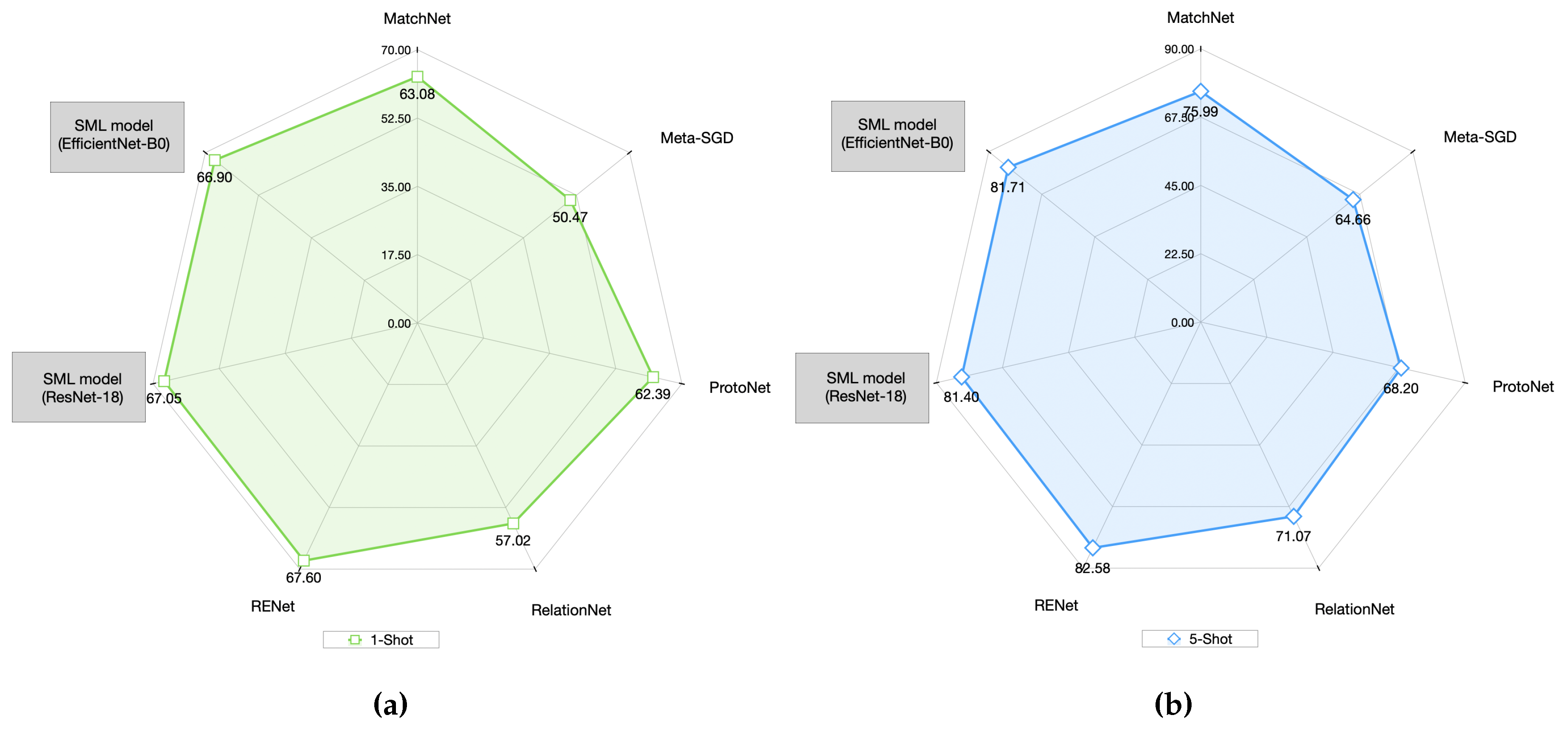
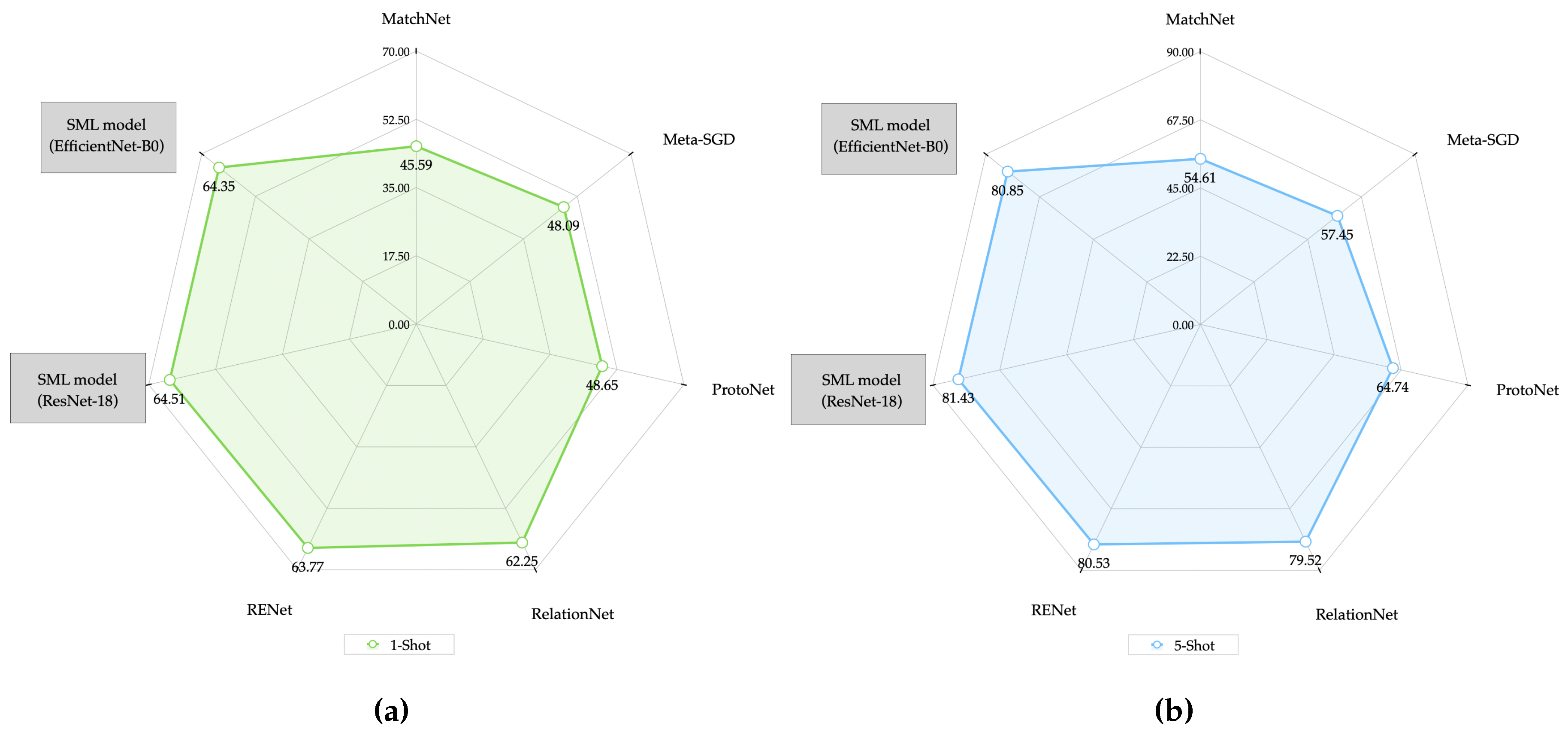
Graphically in Figure 13 it can be seen that the proposed SML model for the MiniImageNet dataset in 1-Shot mode and as an EfficientNet-B0 feature extractor, performs better than all models except RENet, which was better by 1.04 % . Similarly in performance for the 5-Shot mode (Figure 13), the model RENet was also 1.06 % better than the SML model. Therefore, RENet was the model that presented the best result for both modes (1-Shot and 5-Shot) of the comparative models using the MiniImageNet dataset.
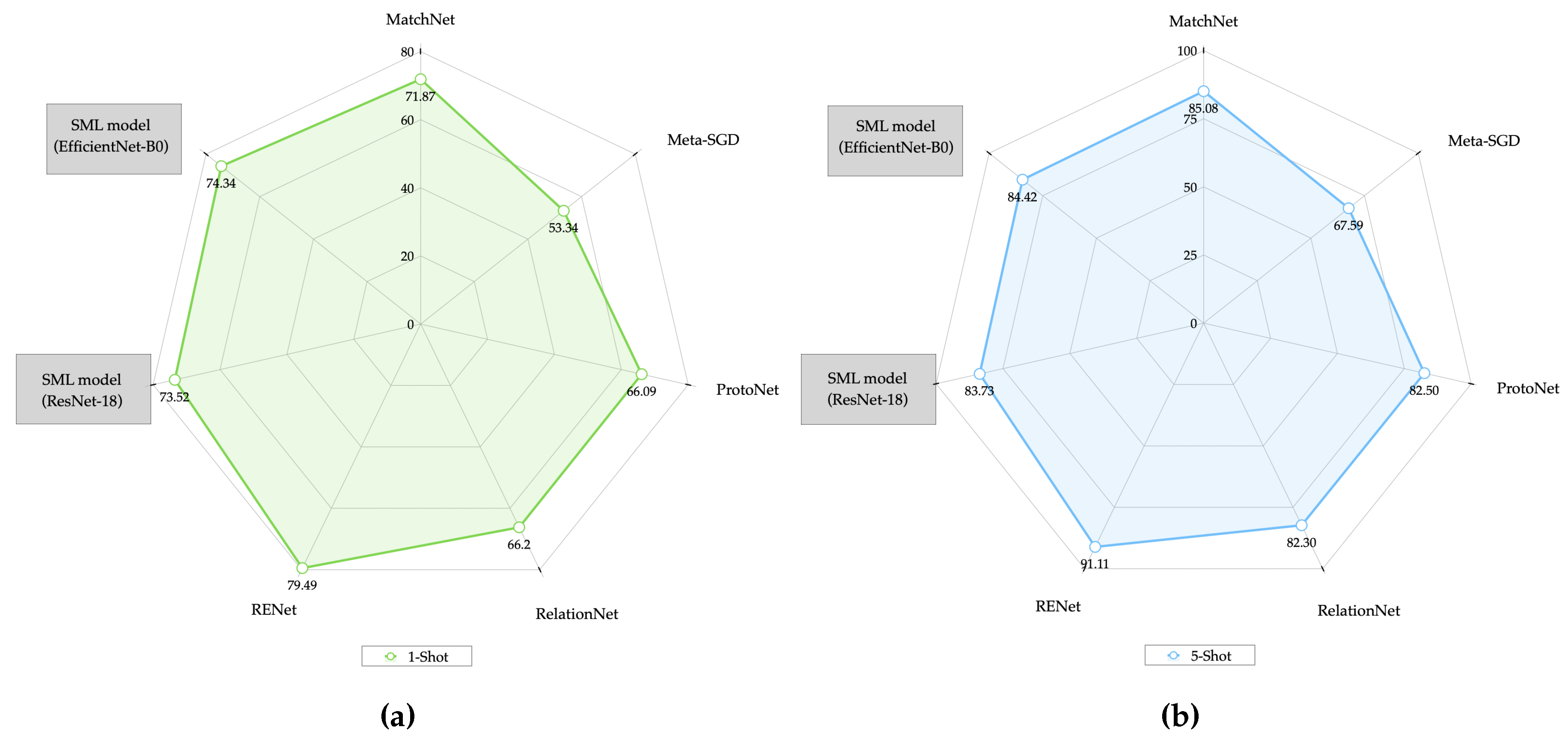
Similarly, in Figure 14b,b it can be observed that for the CUB-200-2011 dataset, the SML model in both modes (1-Shot and 5-Shot) did not have an average precision as close to the RENet model, since the latter was better by 6.93 % and 7.92 % for the 1-Shot and 5-Shot modes respectively.
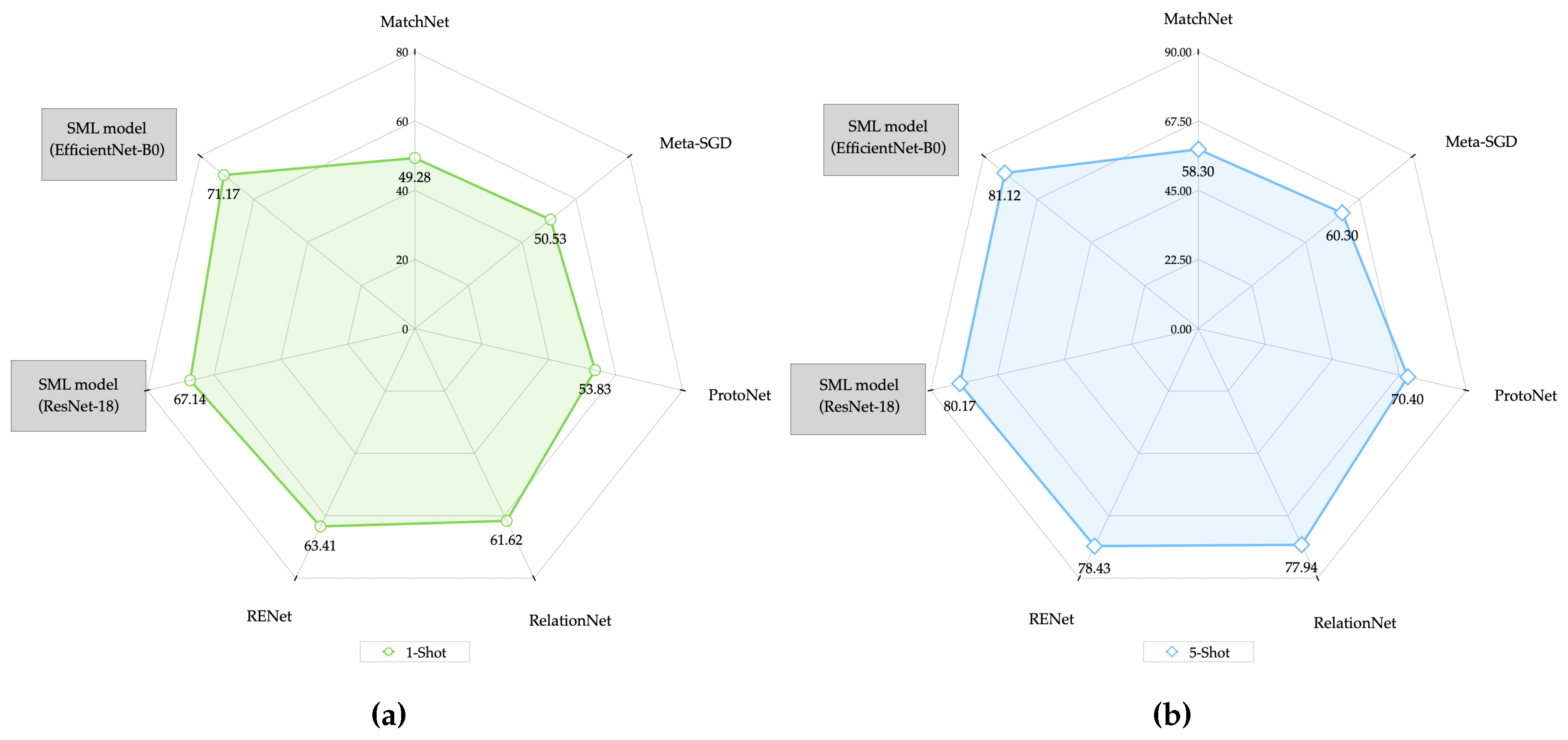
Continuing with the results obtained, Figure 15a,b show us how the SML model using the CIFAR-100 dataset and when compared with the state-of-the-art models, surpassed the Dual Trinet model on average in accuracy by 12.24 % in 1-Shot mode and by 3.43 % in 5-Shot mode to the model, whose results had been the best as observed in Table 6.
Finally, for the DroNet dataset, as can be seen in Figure 16, the SML model using the 1-Shot mode outperforms the Dual Trinet model by only 0.91 % , the latter being the model that presented the best average accuracy of the analyzed models for that particular mode. Similarly, the Dual Trinet model for the 5-Shot mode was outperformed by our SML model in average accuracy but only by 0.40 % as seen in Figure 16.
The above results allow us to conclude that our SML model compared to the state-of-the-art models, using two of the data sets (CIFAR-100 and DroNet), has a better performance and generalization in the 1-Shot and 5-Shot mode using both the ResNet-18 and EfficientNet-B0 feature extractors. However, for the MiniImageNet and CUB-200-2011 data sets, results close to the RENet model were obtained, which was the one that obtained the best results in terms of average accuracy.

5. Discussion

As shown in this previous section, in the experiments carried out with the described data sets and the CNN networks, the proposed Siamese network model was able to perform better in the One-Shot and 5-Shot learning methods. Because the ResNet-18 CNN learns from residuals and as shown in [34], it is a practical feature extractor for one-shot learning tasks. It could also be seen that its demonstrated classification accuracy was very close to EfficientNet-B0 and was consistent with the CNNs that have been used for comparison.
It can also be observed that when classifying new data with the experimental models, the accuracy within the classification decreases and this is due to the change in the distribution of the data present in the dataset. Although the data used in One-Shot learning comes from disjoint classes, they all present and come from the same data distribution. Likewise, based on the work presented in [30], we present that the accuracy demonstrated in the classification of our model using the CNNs ResNet-18 CNN and EfficientNet-B0, which have been trained with the MiniImagenet dataset and validated with the CIFAR-100 and DroNet data sets, and the classification accuracy is presented in Table 6 and Table 7 with 95% confidence.
Our experimental phase with the datasets and CNNs networks resulted in our proposed model performing better in classification accuracy than other 1-Shot learning methods that use the cosine function as a similarity layer. As shown in particular, our Siamese network model when using the ResNet-18 feature extractor had better performance than when using EfficientNet-B0 for the MiniImageNet dataset. Architectures with fewer parameters were used, similar to those used in [34] and [22]. It should be noted that the performance of our model is due to the fused affinity layer (bi-layer) that was developed and it is also emphasized that the careful combination of the affinity layers allowed us to have a significant improvement in the classification accuracy in 1-Shot and 5-Shot learning tasks.

6. Conclusions

Feature detection, accuracy, and learning speed represent three of the most important problems in the field of machine learning systems. These systems, in many real-world scenarios, will operate in unstructured environments and will therefore require architectures that can adapt to variations and perturbations in those environments.
The Siamese artificial neural network model that is proposed as a solution to automatically recognize a possible collision risk for a cyclist within the urban environment is basically based on two layers of affinity, resembling human contrastive learning, to perform the Few-Shot learning task. The results generated experimentally demonstrate that the proposed model performs better and above the baseline set by almost all models in the state of the art using the aforementioned data sets.
It was also observed that our Siamese artificial neural network model produces results whose consistency is compared to other feature extraction networks, but using a smaller size in the example data set for training. One of the main results has been to demonstrate that the proposed SML model works in a comparable manner and in some cases above the baseline established by the Siamese network models in the state of the art, using similar data sets as well as specific data for the problem at hand. This allows us to infer that the technological tool developed in this research can be considered as an applicable partial solution.
Finally we can mention that this is a work in progress whose usefulness can be extended to various fields of application and whose components can be improved as the research advances, such as feature extractors with better performance, faster and greater precision.

Funding

The authors are thankful for the financial support of the projects to the Secretería de Investigación y Posgrado del Instituto Politécnico Nacional with grant numbers: 20220268, 20232264, 20221089 and 20232570, as well as the support from Comisión de Operación y Fomento de Actividades Académicas, BEIFI Program and Consejo Nacional de Humanidades Ciencia y Tecnología (CONAHCYT).

Conflicts of Interest

The authors declare no conflicts of interest.

Abbreviations

The following abbreviations are used in this manuscript:
CNN Convolutional Neural Network
CNNs Convolutional Neural Networks
DL Deep Learning
LSTM Long Short-Term Memory
ML Machine Learning
SML Simplified Machine Learning

References

  1. López Gómez, L. La bicicleta como medio de transporte en la movilidad sustentable. Technical report, Dirección General de Análisis Legislativo, Senado de la República, México, 2018.
  2. ITDP. Manual Ciclociudades I. La Movilidad en Bicicleta como Política Pública. In Manual Ciclociudades; Instituto de Políticas para el Transporte y el Desarrollo: México D.F., 2011; Vol. I, p. 62.
  3. Vision Zero Network. What is Vision Zero? 2022. Available online: https://visionzeronetwork.org/about/what-is-vision-zero/.
  4. WHO. Global status report on road safety 2018. Technical report, World Health Organization, Geneva, 2018.
  5. INEGI. Estadísticas a propósito del Día de Muertos, DATOS NACIONALES. Technical report, Instituto Nacional de Estadística y Geografía, México, 2019.
  6. Hilmkil, A.; Ivarsson, O.; Johansson, M.; Kuylenstierna, D.; van Erp, T. Towards Machine Learning on data from Professional Cyclists. 2018; arXiv:cs.LG/1808.00198]. [Google Scholar]
  7. Ngiam, J.; Khosla, A.; Kim, M.; Nam, J.; Lee, H.; Ng, A.Y. Multimodal Deep Learning. In Proceedings of the Proceedings of the 28th International Conference on Machine Learning, ICML 2011, Bellevue, Washington, USA, June 28 - July 2, 2011; Getoor, L.; Scheffer, T., Eds. Omnipress. 2011; 689–696. [Google Scholar]
  8. Srivastava, N.; Salakhutdinov, R. Multimodal Learning with Deep Boltzmann Machines. J. Mach. Learn. Res. 2014, 15, 2949–2980. [Google Scholar]
  9. Zhao, H.; Wijnands, J.S.; Nice, K.A.; Thompson, J.; Aschwanden, G.D.P.A.; Stevenson, M.; Guo, J. Unsupervised Deep Learning to Explore Streetscape Factors Associated with Urban Cyclist Safety. In Proceedings of the Smart Transportation Systems 2019; Qu, X.; Zhen, L.; Howlett, R.J.; Jain, L.C., Eds., Singapore. 2019; pp. 155–164. [Google Scholar]
  10. Galán, R.; Calle, M. García., J.M. Análisis de variables que influencian la accidentalidad ciclista: desarrollo de modelos y diseño de una herramienta de ayuda. In Proceedings of the XIII Congreso de Ingeniería de Organización Barcelona-Terrassa, September 2nd-4th 2009. Asociación para el Desarrollo de la Ingeniería de Organización - ADINGOR. 2009; 696–703. [Google Scholar]
  11. Caterini, A.L.; Chang, D.E. Deep Neural Networks in a Mathematical Framework, 1st ed.; Springer Publishing Company, Incorporated, 2018.
  12. Cuomo, S.; Di Cola, V.S.; Giampaolo, F.; Rozza, G.; Raissi, M.; Piccialli, F. Scientific Machine Learning Through Physics–Informed Neural Networks: Where we are and What’s Next. Journal of Scientific Computing 2022, 92, 88. [Google Scholar] [CrossRef]
  13. Khosla, P.; Teterwak, P.; Wang, C.; Sarna, A.; Tian, Y.; Isola, P.; Maschinot, A.; Liu, C.; Krishnan, D. Supervised Contrastive Learning. 2021; arXiv:cs.LG/2004.11362. [Google Scholar]
  14. Chen, T.; Kornblith, S.; Norouzi, M.; Hinton, G. A Simple Framework for Contrastive Learning of Visual Representations. In Proceedings of the Proceedings of the 37th International Conference on Machine Learning; III, H.D.; Singh, A., Eds. PMLR, 13–18 Jul 2020, Vol. 119, Proceedings of Machine Learning Research. 1597–1607.
  15. van den Oord, A.; Li, Y.; Vinyals, O. Representation Learning with Contrastive Predictive Coding. 2019; arXiv:cs.LG/1807.03748. [Google Scholar]
  16. Tian, Y.; Krishnan, D.; Isola, P. Contrastive Multiview Coding. 2020; arXiv:cs.CV/1906.05849. [Google Scholar]
  17. Hjelm, R.D.; Fedorov, A.; Lavoie-Marchildon, S.; Grewal, K.; Bachman, P.; Trischler, A.; Bengio, Y. Learning deep representations by mutual information estimation and maximization. In Proceedings of the International Conference on Learning Representations. 2019. [Google Scholar]
  18. He, K.; Fan, H.; Wu, Y.; Xie, S.; Girshick, R. Momentum Contrast for Unsupervised Visual Representation Learning. In Proceedings of the 2020 IEEE/CVF Conference on Computer Vision and Pattern Recognition (CVPR). 2020; 9726–9735. [Google Scholar] [CrossRef]
  19. Hernández-Herrera, A.; Espino, E.R.; Álvarez Vargas, R.; Ponce, V.H.P. Una Exploración Sobre el Aprendizaje Automático Simplificado: Generalización a partir de Algunos Ejemplos. Komputer Sapiens 2021, 3, 36–41. [Google Scholar]
  20. Lee, S.W.; O’Doherty, J.P.; Shimojo, S. Neural Computations Mediating One-Shot Learning in the Human Brain. PLOS Biology 2015, 13, 1–36. [Google Scholar] [CrossRef] [PubMed]
  21. Snell, J.; Swersky, K.; Zemel, R. Prototypical Networks for Few-shot Learning. In Proceedings of the Advances in Neural Information Processing Systems; Guyon, I.; Luxburg, U.V.; Bengio, S.; Wallach, H.; Fergus, R.; Vishwanathan, S.; Garnett, R., Eds. Curran Associates, Inc. 2017; 30. [Google Scholar]
  22. Vinyals, O.; Blundell, C.; Lillicrap, T.; kavukcuoglu, k.; Wierstra, D. Matching Networks for One Shot Learning. In Proceedings of the Advances in Neural Information Processing Systems; Lee, D.; Sugiyama, M.; Luxburg, U.; Guyon, I.; Garnett, R., Eds. Curran Associates, Inc. 2016; 29. [Google Scholar]
  23. y Christian Paulina Mendoza Torres, R.H.S. Metodología de la Investigación: Las rutas cuantitativa, cualitativa y mixta; McGraw-Hill Interamericana, 2018.
  24. Xing, E.; Jordan, M.; Russell, S.J.; Ng, A. Distance Metric Learning with Application to Clustering with Side-Information. In Proceedings of the Advances in Neural Information Processing Systems; Becker, S.; Thrun, S.; Obermayer, K., Eds. MIT Press. 2002; 15. [Google Scholar]
  25. Hadsell, R.; Chopra, S.; LeCun, Y. Dimensionality Reduction by Learning an Invariant Mapping. In Proceedings of the 2006 IEEE Computer Society Conference on Computer Vision and Pattern Recognition (CVPR’06). 2006; 2, 1735–1742. [Google Scholar] [CrossRef]
  26. Bromley, J.; Bentz, J.W.; Bottou, L.; Guyon, I.M.; LeCun, Y.; Moore, C.; Säckinger, E.; Shah, R. Signature Verification Using A "Siamese" Time Delay Neural Network. Int. J. Pattern Recognit. Artif. Intell. 1993, 7, 669–688. [Google Scholar] [CrossRef]
  27. Koch, G.R. Siamese Neural Networks for One-Shot Image Recognition. In Proceedings of the Proceedings of the 32nd International Conference on Machine Learning; 2015. [Google Scholar]
  28. He, K.; Zhang, X.; Ren, S.; Sun, J. Deep residual learning for image recognition. In Proceedings of the Proceedings of the IEEE conference on computer vision and pattern recognition. 2016; pp. 770–778. [Google Scholar]
  29. Tan, M.; Le, Q. Efficientnet: Rethinking model scaling for convolutional neural networks. In Proceedings of the International conference on machine learning. PMLR. 2019; pp. 6105–6114. [Google Scholar]
  30. Li, X.; Yu, L.; Fu, C.W.; Fang, M.; Heng, P.A. Revisiting metric learning for few-shot image classification. Neurocomputing 2020, 406, 49–58. [Google Scholar] [CrossRef]
  31. Krizhevsky, A.; Hinton, G. Learning multiple layers of features from tiny images. Technical Report 0, University of Toronto, Toronto, Ontario, 2009.
  32. Wah, C.; Branson, S.; Welinder, P.; Perona, P.; Belongie, S. The Caltech-UCSD Birds-200-2011 Dataset; 2011.
  33. Loquercio, A.; Maqueda, A.I.; del Blanco, C.R.; Scaramuzza, D. DroNet: Learning to Fly by Driving. IEEE Robotics and Automation Letters 2018, 3, 1088–1095. [Google Scholar] [CrossRef]
  34. Chen, Z.; Fu, Y.; Zhang, Y.; Jiang, Y.G.; Xue, X.; Sigal, L. Multi-Level Semantic Feature Augmentation for One-Shot Learning. IEEE Transactions on Image Processing 2019, 28, 4594–4605. [Google Scholar] [CrossRef]
  35. Sung, F.; Yang, Y.; Zhang, L.; Xiang, T.; Torr, P.H.; Hospedales, T.M. Learning to Compare: Relation Network for Few-Shot Learning. In Proceedings of the 2018 IEEE/CVF Conference on Computer Vision and Pattern Recognition; 2018; pp. 1199–1208. [Google Scholar] [CrossRef]
  36. Hilliard, N.; Phillips, L.; Howland, S.; Yankov, A.; Corley, C.D.; Hodas, N.O. Few-Shot Learning with Metric-Agnostic Conditional Embeddings. 2018; arXiv:cs.LG/1802.04376. [Google Scholar]
  37. Zhou, F.; Wu, B.; Li, Z. Deep Meta-Learning: Learning to Learn in the Concept Space. ArXiv 2018, abs/1802.03596.
  38. Mangla, P.; Kumari, N.; Sinha, A.; Singh, M.; Krishnamurthy, B.; Balasubramanian, V.N. Charting the Right Manifold: Manifold Mixup for Few-shot Learning. In Proceedings of the Proceedings of the IEEE/CVF Winter Conference on Applications of Computer Vision (WACV), March 2020.
  39. Kang, D.; Kwon, H.; Min, J.; Cho, M. Relational Embedding for Few-Shot Classification. In Proceedings of the Proceedings of the IEEE/CVF International Conference on Computer Vision (ICCV), October. 2021; 8822–8833. [Google Scholar]
  40. Li, Z.; Zhou, F.; Chen, F.; Li, H. Meta-SGD: Learning to Learn Quickly for Few-Shot Learning. 2017; arXiv:cs.LG/1707.09835. [Google Scholar]
  41. Finn, C.; Abbeel, P.; Levine, S. Model-Agnostic Meta-Learning for Fast Adaptation of Deep Networks. In Proceedings of the Proceedings of the 34th International Conference on Machine Learning; Precup, D.; Teh, Y.W., Eds. PMLR, 06–11 Aug 2017, Vol. 70, Proceedings of Machine Learning Research. pp. 1126–1135.
Figure 1. Urban mobility hierarchy (adapted from [2]).
Preprints 143477 g001
Figure 2. Intuitive features that proposed machine learning model should be able to handle.
Preprints 143477 g002
Figure 3. Contrast Losses. Self-supervised contrast loss contrasts a single positive image for each anchor (i.e., a magnified version of the same image) with a set of negative images from the sample set (Figure 3). However, the supervised contrast loss (Figure 3) considered in this article, contrasts the set of all samples of the same class as positive with the negative ones of the rest of the set of images. As the condor photo demonstrates, taking the class label information into account results in a representation space (embedding space) where elements of the same class are more aligned than in the self-supervised case.
Preprints 143477 g003
Figure 4. Learn new information based on some prior knowledge.
Preprints 143477 g004
Figure 5. General methodology and research development.
Preprints 143477 g005
Figure 6. Schematic diagram of the Siamese network.
Preprints 143477 g006
Figure 7. The architecture of the Siamese Cognitive Model. The model feeds, through the input images, the extraction of features using CNNs. The outputs are two feature vectors that are passed to the affinity layers A 1 and A 2 . They are then integrated into the combined affinity layer (bi-layer), where the maximum affinity is calculated. The output of the combined affinity layer is passed through the activation function to determine the similarity or dissimilarity between the inputs.
Preprints 143477 g007
Figure 8. An example about the precision of five random sample images in single example (1-Shot) mode. The maximum predicted affinity score is indicated in the fourth row (boxed), which approximates the correct prediction of a value equal to 1 (affinity images), therefore, this would represent a correct prediction of the model.
Preprints 143477 g008
Figure 9. Comparison with reference data. Performance results with different datasets using ResNet-18 feature extractor.
Preprints 143477 g009
Figure 10. ResNet-18 Summary. Comparative summary of average accuracy with the different datasets.
Preprints 143477 g010
Figure 11. Comparison with reference data. Performance results with different datasets using the EfficientNet-B0 feature extractor.
Preprints 143477 g011
Figure 12. EfficientNet-B0 Summary. Comparative summary of average accuracy with the different datasets.
Preprints 143477 g012
Figure 13. Performance between the state-of-the-art models and the proposed model (SML) using the MiniImageNet dataset. In 1-Shot (Figure 13) and 5-Shot mode (Figure 13).
Preprints 143477 g013
Figure 14. Performance between the state-of-the-art models and the proposed model (SML) using the CUB-200-2011 dataset. In 1-Shot (Figure 14) and 5-Shot mode (Figure 14).
Preprints 143477 g014
Figure 15. Performance between the state-of-the-art models and the proposed model (SML) using the CIFAR-100 dataset. In 1-Shot (Figure 15) and 5-Shot mode (Figure 15).
Preprints 143477 g015
Figure 16. Performance between the state-of-the-art models and the proposed model (SML) using the DroNet dataset. In 1-Shot (Figure 16) and 5-Shot mode (Figure 16).
Preprints 143477 g016
Table 1. Intuitive information that is observed in the problem analysis.
Available Not Available
Position Types of possible moving obstacles
Orientation Number of moving obstacles
Velocity Position of moving obstacles
Aceleration Known data set according to the problem for analysis and testing.
Image / Video
Table 2. Identification accuracy. Average accuracy results with 95% confidence of the four datasets against three different affinity methods ( A 1 , A 2 and proposed SML model) using ResNet-18 as feature extractor. All experiments with the proposed model with maximum affinity layer A m a x are highlighted in bold.
Feature extractor Dataset A1 A2 SML model ( A max )
    1-Shot 5-Shot 1-Shot 5-Shot 1-Shot 5-Shot
ResNet-18 MiniImageNet 62.93 69.66 62.86 67.66 67.05 81.40
  CIFAR-100 62.83 68.50 64.30 67.99 67.14 80.17
  CUB-200–2011 70.46 77.29 70.48 76.32 73.52 83.73
  DroNet 59.93 66.56 59.28 63.07 64.51 80.85
Table 3. Identification accuracy. Average accuracy results with 95% confidence of the four datasets against three different affinity methods ( A 1 , A 2 and proposed SML model) using EfficientNet-b0 as feature extractor. All experiments with maximum affinity layer A m a x are highlighted in bold.
Feature extractor Dataset A1 A2 SML model ( A max )
    1-Shot 5-Shot 1-Shot 5-Shot 1-Shot 5-Shot
EfficientNet-b0 MiniImageNet 64.14 70.47 61.65 64.49 66.90 81.71
  CIFAR-100 68.72 73.59 66.95 68.99 71.17 79.12
  CUB-200–2011 73.58 80.38 71.83 76.90 74.34 84.42
  DroNet 61.99 69.14 60.08 64.28 64.35 80.85
Table 4. Comparison with the state of the art using MiniImageNet. The accuracy between the state-of-the-art models and the SML proposed model is presented using the MiniImageNet dataset. Columns show the name of the model used, the feature extractor, the dataset, and the two k-shot learning modes used. The best results with our model are highlighted in bold.
Model Feature extractor MiniImageNet
    1-Shot 5-Shot
[22] MatchNet ResNet-12 63.08 75.99
[40] Meta-SGD ResNet-50 50.47 64.66
[21] ProtoNet ResNet-12 62.39 68.20
[35] RelationNet ResNet-34 57.02 71.07
[39] RENet ResNet-12 67.60 82.58
SML (Our model) ResNet-18 67.05 81.40
SML (Our model) EfficientNet-B0 66.90 81.71
Table 5. Comparison with the state of the art using CUB-200–2011. The accuracy between the state-of-the-art models and the SML proposed model is presented using the MiniImageNet dataset. Columns show the name of the model used, the feature extractor, the dataset, and the two k-shot learning modes used. The best results with our model are highlighted in bold.
Model Feature extractor CUB-200–2011
    1-Shot 5-Shot
[22] MatchNet ResNet-12 71.87 85.08
[40] Meta-SGD ResNet-50 53.34 67.59
[21] ProtoNet ResNet-12 66.09 82.50
[35] RelationNet ResNet-34 66.20 82.30
[39] RENet ResNet-12 79.49 91.11
SML (Our model) ResNet-18 73.52 83.73
SML (Our model) EfficientNet-B0 74.34 84.42
Table 6. Comparison with the state of the art using CIFAR-100. The accuracy between the state-of-the-art models and the SML proposed model is presented using the MiniImageNet dataset. Columns show the name of the model used, the feature extractor, the dataset, and the two k-shot learning modes used. The best results with our model are highlighted in bold.
Model Feature extractor CIFAR-100
    1-Shot 5-Shot
[41] MAML ResNet-12 49.28 58.30
[22] MatchNet ResNet-12 50.53 60.30
[40]Meta-SGD ResNet-50 53.83 70.40
[37]DEML+Meta-SGD ResNet-50 61.62 77.94
[34]Dual TriNet ResNet-18 63.41 78.43
SML (Our model) ResNet-18 67.14 80.17
SML (Our model) EfficientNet-B0 71.17 81.12
Table 7. Comparison with the state of the art using DroNet. The accuracy between the state-of-the-art models and the SML proposed model is presented using the MiniImageNet dataset. Columns show the name of the model used, the feature extractor, the dataset, and the two k-shot learning modes used. The best results with our model are highlighted in bold.
Model Feature extractor DroNet
    1-Shot 5-Shot
[41] MAML ResNet-12 45.59 54.61
[22] MatchNet ResNet-12 48.09 57.45
[40]Meta-SGD ResNet-50 48.65 64.74
[37]DEML+Meta-SGD ResNet-50 62.25 79.52
[34]Dual TriNet ResNet-18 63.77 80.53
SML (Our model) ResNet-18 64.51 81.43
SML (Our model) EfficientNet-B0 64.35 80.85
Disclaimer/Publisher’s Note: The statements, opinions and data contained in all publications are solely those of the individual author(s) and contributor(s) and not of MDPI and/or the editor(s). MDPI and/or the editor(s) disclaim responsibility for any injury to people or property resulting from any ideas, methods, instructions or products referred to in the content.
Copyright: This open access article is published under a Creative Commons CC BY 4.0 license, which permit the free download, distribution, and reuse, provided that the author and preprint are cited in any reuse.
Prerpints.org logo

Preprints.org is a free preprint server supported by MDPI in Basel, Switzerland.

Subscribe

Disclaimer

Terms of Use

Privacy Policy

Privacy Settings

© 2025 MDPI (Basel, Switzerland) unless otherwise stated