Submitted:
12 May 2025
Posted:
12 May 2025
Read the latest preprint version here
Abstract
Conditional Value-at-Risk (CVaR) is one of the most popular risk measures in finance, used in risk management as a complementary measure to Value-at-Risk (VaR). VaR estimates potential losses within a given confidence level, such as 95% or 99%, but does not account for tail risks. CVaR addresses this gap by calculating the expected losses exceeding the VaR threshold, providing a more comprehensive risk assessment for extreme events. This research explores the application of Denoising Diffusion Probabilistic Models (DDPM) to enhance CVaR calculations. Traditional CVaR methods often fail to capture tail events accurately, whereas DDPMs generate a wider range of market scenarios, improving the estimation of extreme risks. However, these models require significant computational resources and may present interpretability challenges.
Keywords:
CVaR
; finance
; risk management
; VaR
; deep learning
; generative models
; denoising diffusion probabilistic models
1. Introduction
In modern financial industry, management of financial risk is one of the key tasks for companies, banks and investors. To estimate how big losses could be dangerous, tools like Conditional Value at Risk and Values at Risk have been used for a long time. They are the most popular, because could give understandable number type risk assess.
The last crisis events - like crisis in 2008 and economic shock of Covid-19 showed that the traditional methods cannot be safe. Most hard they cannot calculate unstable situations, when situation on the market is out of control.
Conditional Value at Risk(CVaR) - more deep version of VaR. If VaR tells, what loss will not be more than some amount of confidence, so CVaR answers, what if will we have the extreme situation, how many we will lose. That is why CVaR more usable in tasks, where need to count extreme risks, not only average loss.
Problem of the traditional methods of calculating of CVaR - like Historical Simulation and Monte-Carlo modelling are built on assumption, which are not always being on real life. For example, often assumed, that distribution of returns are normal and not effect to each other. On practice the market being more difficult.
With the development of machine learning opens new ability to modelling financial data. Especially interesting is Diffusion Probabilistic Models(DDPM). These models are able to step by step unlearn the process of data noise and restore complex patterns to the original data.
On the start DDPM mostly used for generating image, but their idea more useful also in finance. They can create artificial returns, which is better can show rear events and extreme losses.
In this work we will discuss, how we could use DDPM for calculating CVaR, by comparing result with traditional methods. Our goal - show, that the modern generative models could calculate risks more accurate, especially in volatile markets.
2. Literature Review
A lot of years financial risk assessment use metrics like Value-at-Risk(VaR) and Conditional Value at Risk(CVaR). But traditional methods of calculating often work bad, especially when market is unstable - for example crisis time. It depends on that they rely on simplified assumptions, like the profit conditions are normal, but in real that is not.
In Cont’s(2001) work deeply discussed about real features of returns - that called “stylized facts”: tail risks, autocorrelation, high volatility and others. These characteristics are interfere to use standard models, because they not include, how market could be unstable[10]. So, to solve that problems, started to use machine learning. For example, Fatouros et al.(2022) offered DeepVar model - it is neural network, which could predict VaR for the portfolio. Their results shows, their way could get more accurate risk assess, especially volatility time[4].
Other interested idea - use quantile regression with generative models. In Wang et al.(2024) firstly calculate VaR with regression, then with LSGAN(one of the GAN type) creating possible negative scenarios, for calculate ES. Result was better, than classical methods.[1].
Other way, starts to use Variational Autoencoder(VAE). In Sicks(2021) and Buch’s(2023) works shows, how VAE could be use for VaR assess, if consider time series. They teach the model on real data and show, that the model can generate possible scenarios, including rare events[2,3].
Later created Diffusion Models, as Denoising Diffusion Probabilistic Models(DDPM). It is models which teaches “cancel the noise”, step by step restore the data, then Rasul et al.(2021) adapted ut under the time series - TimeGrad model[5,6]. Comparing these methods shows in Bond-Taylor et al(2021) review. It discussed, that the DDPM is one of the more accurate and stable generative method. It better than GAN and VAE, in tail distribution work, that is with rare and dangerous events[7].
Also Tobjork(2021) have interesting work, where he tried to use GAN for VaR assessment. He showed, that is work, but that models not always stable and may get stuck in the same scenario[8].
For check the result of risk assessment and how the model is working we have a special tests. One of the most popular - test of Acerbi and Szekely(2014). It helps understand, how good and correct models calculate not only VaR and also CVaR(losses in worst situations)
2.1. Difference of My Work
Much models required to do hard assumptions about market or have a bad deal with rare situations. In my work i use Diffusion Model, which adapted under a financial data. It does not rely on fixed assumption and could generate scenarios with rare, but important events. Difference of my method with other that my method aims to accurate CVaR calculation, not just generate data and calculate quantile. It makes the method more safe in stressful situation.
2.2. Features of the Project
This project explores a data-driven approach to risk estimation using generative models, and in particular, for CVaR estimation. Unlike more traditional methods relying on pre-specified statistical formulas or hypotheses about return distribution shapes, this model learns from data directly and generates realistic future scenarios. One of the advantages is that it does not assume returns must be normally distributed — it builds its forecasts from what is actually seen.
The method is based on a diffusion model (DDPM), adapted to work with time series. That allows it to generate not only random samples, but entire return paths given history. That makes the model closer to the way real financial data actually does behave over time. Specific attention is paid to the detection and reproduction of unusual and rare occurrences — the kind of occurrence the usual models are likely to miss but which can lead to the largest losses.
To assess the effectiveness of the model, its performance is compared against two popular baseline techniques: historical simulation and Monte Carlo. This comparison indicates where the generative method provides enhancements, especially in terms of tail risk capture. The internal parameters of the model (such as the number of diffusion steps or learning rate) are optimized with automated search algorithms like Optuna, ensuring efficiency and reproducibility.
Finally, to facilitate easier interpretation of the findings, the project includes simple visualizations — showing return distributions, VaR and CVaR levels, and frequencies at which actual outcomes fall outside expected ranges. These graphs provide a way to make the technical work reflect useful insights that can be transferred in practical financial risk analysis.
2.3. Goal of the Project
The main goal of this project is to improve the way financial risk is assessed by using modern generative models. More specifically, the project focuses on estimating Conditional Value-at-Risk (CVaR) with the help of a diffusion-based neural network. Traditional methods often rely on simplified assumptions about market behavior, which can lead to inaccurate estimates, especially during periods of high volatility or extreme market events.
By generating possible future return scenarios rather than just forecasting single-point values, the model aims to better capture tail risks — the rare but impactful outcomes that are crucial for decision-making in finance. The project also compares this approach with established methods like historical simulation and Monte Carlo, to highlight the advantages and limitations of each.
The long-term objective is to offer a more flexible, data-driven alternative for risk analysis — one that adapts to real-world financial data without depending on fixed distributional assumptions.
3. Technical and Analytical Evaluation
3.1. Data Preprocessing
For this work were used historical data of S&P500 assets, data was taken from open source platform(Kaggle). From all pack of tickets has chosen only 3 companies: Apple(AAPL), Microsoft(MSFT),Amazon(AMZN). All of this companies have a high level of correlation because they are technical giants. After upload the data, it will be sorted by data and ticker. The main variable that was used was the logarithmic daily income. It was calculated using the formula:
This form better reflects relative price changes and eliminates large-scale difference between stocks. Then needed to change the format for easy to work in multidimensional time series, changes: rows - data, columns - tickers, values - counted returns. In result the table, where every rows are the vector of the return on four assets for given day.
Then were deleted with passed values. It is important, on all assets for the every moment of the time data will be synchronized and full.
To speed up and simplify model’s learning, data was reduced to a single scale using standard z-transform. It deleted the bias toward assets with more volatility.
To feed the data into the model, the data was split into overlapping 30-day windows. Each such window represents a multidimensional time slice that includes returns on all assets. These windows are used in training as single examples, allowing the model to capture time dependencies and dynamics within each sequence.
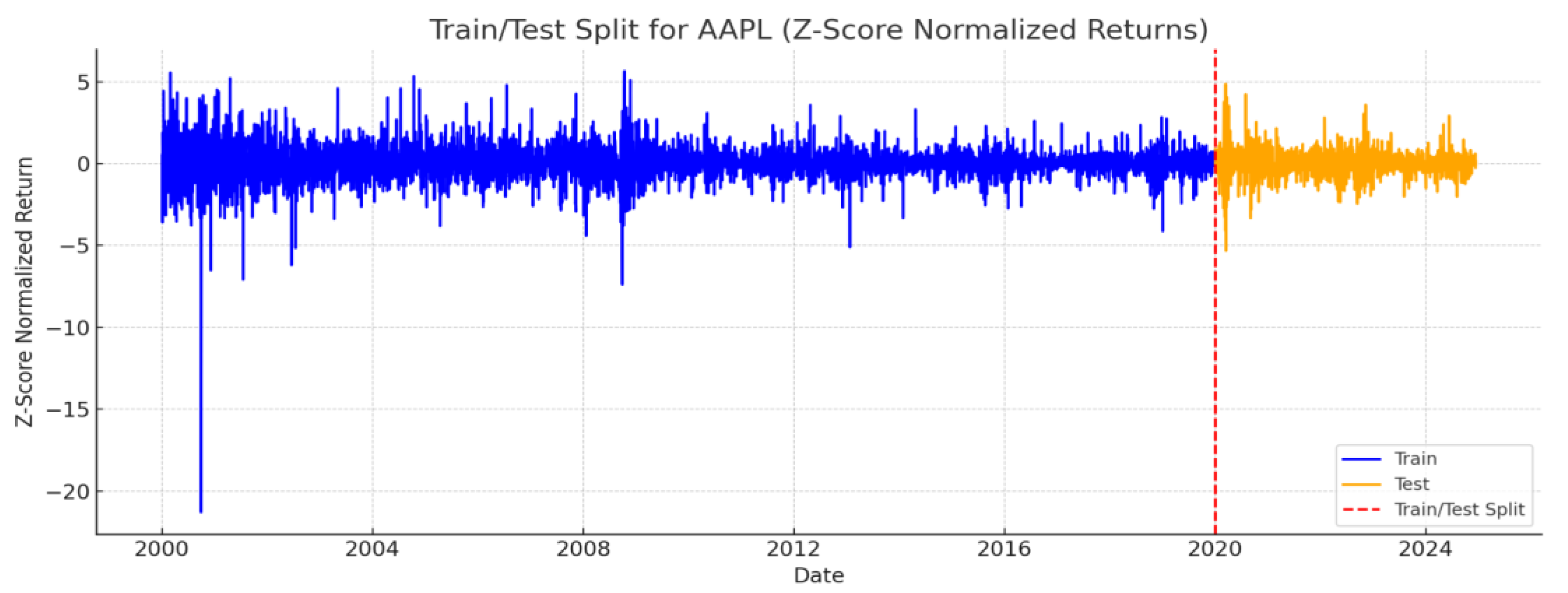
The data was split in an 80/20 ratio. At the same time, the chronology was observed.: first the training part, then the test part.
3.2. Model Architecture
This study employs a denoising diffusion model to generate possible future paths of asset returns. The model is trained on brief time series of daily return data and learns the impact that noise has upon them over time. More importantly, it learns the reversal of that process — taking random noise and converting it back into data that closely resembles previous market activity.
The model receives input as 30-day sequences of returns for three specified stocks: Apple (AAPL), Google (GOOG), and Amazon (AMZN). Thus, each sample has a shape of 30 time steps and 3 features. These sequences are preprocessed and normalized before training.
To handle temporal dependencies, the model uses a Gated Recurrent Unit (GRU) network. This allows it to better capture the dynamics in sequences than a standard feedforward network.
Every input sequence is concatenated with a numeric representation of the present noise level, a method that is also known as "time embedding." The embedding is applied at each time step, enabling the model to adjust in its predictions based on where it is in the diffusion process.
The noise is added with a linear schedule that ramps up noise from a small starting value incrementally over steps. The procedure runs for 1000 steps, where the noise coefficients β range from 0.0001 to 0.02. Incrementally ramping up noise guarantees the model has the ability to learn to denoise even highly degraded inputs.
Traditional models typically make the assumption of a normal distribution for returns or are founded on familiar statistical structures. Diffusion-based models, however, enable: more realistic distributions, such as asymmetry and extreme tails adaptable restoration of uncommon or significant occurrences, and no strong assumptions regarding the form of the data distribution. This positions them favorably for risk modeling, where it is necessary to capture infrequent but significant outcomes.
3.3. Theoretical Background
Short review of key tools:
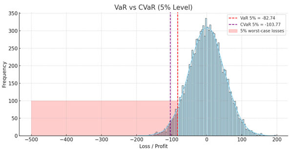
Value-at-Risk(VaR) shows, what losses possible in some of bad X% of cases.
For example: if , that means, in 5% of cases, looses will be worst than 100.
Conditional Value at Risk(CVaR) - it is average losses in worst case scenarios, when the value already exceeded VaR.
Backtesting - it is checking of risk model’s accuracy. For example: compare, how many real losses were higher, than VaR predicted.
Denoising Diffusion Probabilistic Model(DDPM) - generative model, which teaches change a noise to real data, as a daily returns.
TimeGrad - version of DDPM, which knows how to generate sequences(Time Series), it makes it useful in risk assessment tasks
VaR and CVaR definition
VaR in some of confidence level (example: 95%) - it is a number, that with a probability losses will not exceed value. And reverse cases losses will be worst.
The formula (in terms of quantile):
Simplified:
Where X is random value(losses), - level of quantile.
If , so in 5% of worst case scenarios losses will be worse than 100.
CVaR - is average value of losses, in condition, that they already exceeded VaR. That means CVaR looking to the “tail” of assumption and give an expectation in worst case ()% situations.
Formula:
Or, if X - continuous value:
Why CVaR better than VaR:
VaR do not say, how big could be losses, if exceed it.
CVaR takes into account the entire tail of the distribution, and is therefore more reliable.
CVaR often use in regulations, including Basel III.
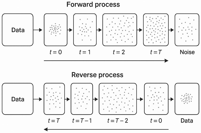
Basics of Diffusion Models(DDPM)
DDPM - is a model, which could step by step add a noise to the data, then teaches to remove it, restoring the initial values.
Forward process(adding a noise):
Reverse process(reverse generation):
Loss-function:
TimeGrad: adaptation DDPM to time series
TimeGrad could generate future values of time series based on previous.
Models works:
- Looks to last k days(example: 90);
- Generates one or couple of possible next values;
- Repeats the process many times(example: 500 times);
-
The obtained trajectories are calculated:
- a.
- VaR - quantile;
- b.
- CVaR - average all values which under the VaR.
4. System Architecture and Design
This section will provide the overall structure of the system used to the model and assess financial risk using DDPM modelling. The system is composed of several key components, from data ingestion to model training, scenario generation and risk evaluation.
4.1. Workflow Overview
The system has a linear pipeline architecture:
Data Acquisition: Historical price data for AAPL, GOOG, and AMZN is retrieved from a structured CSV file.
Preprocessing: Prices are transformed into daily returns and normalized using standard scaling.
Training: A denoising diffusion model based on GRU layers is trained to learn how to denoise return sequences.
Sampling: Once trained, the model is used to generate new return paths by inverting the noise process.
Risk Analysis: The pathways generated are used to estimate the Conditional Value-at-Risk (CVaR) and compared with classical methods.
This arrangement enables the generation of realistic data-based scenarios, which can be utilized for enhanced risk assessment.
4.2. Data Analysis
Taken from open-source platform “Kaggle” dataset of prices of assets from S&P500. Have chosen 3 companies who have a high-level of correlation between each other and have a similar problems in crisis time like COVID-19.
4.3. Return Calculation and Data Cleaning
Asset returns were calculated using this formula:
where is the return at time t and is the adjusted closing price at time .
Data was cleaning using dropna function to delete all empty or NaN values.
4.4. Analysing Dataset
Before proceeding with the development of the models, the dataset was examined closely to determine the overall trends concerning the selected stocks—AAPL, GOOG, and AMZN. As an initial step, I calculated the daily returns using the adjusted closing prices. The computation facilitated the ease of transforming raw price data into percentage change over time, which is more suitable for model development and risk ascertainment.
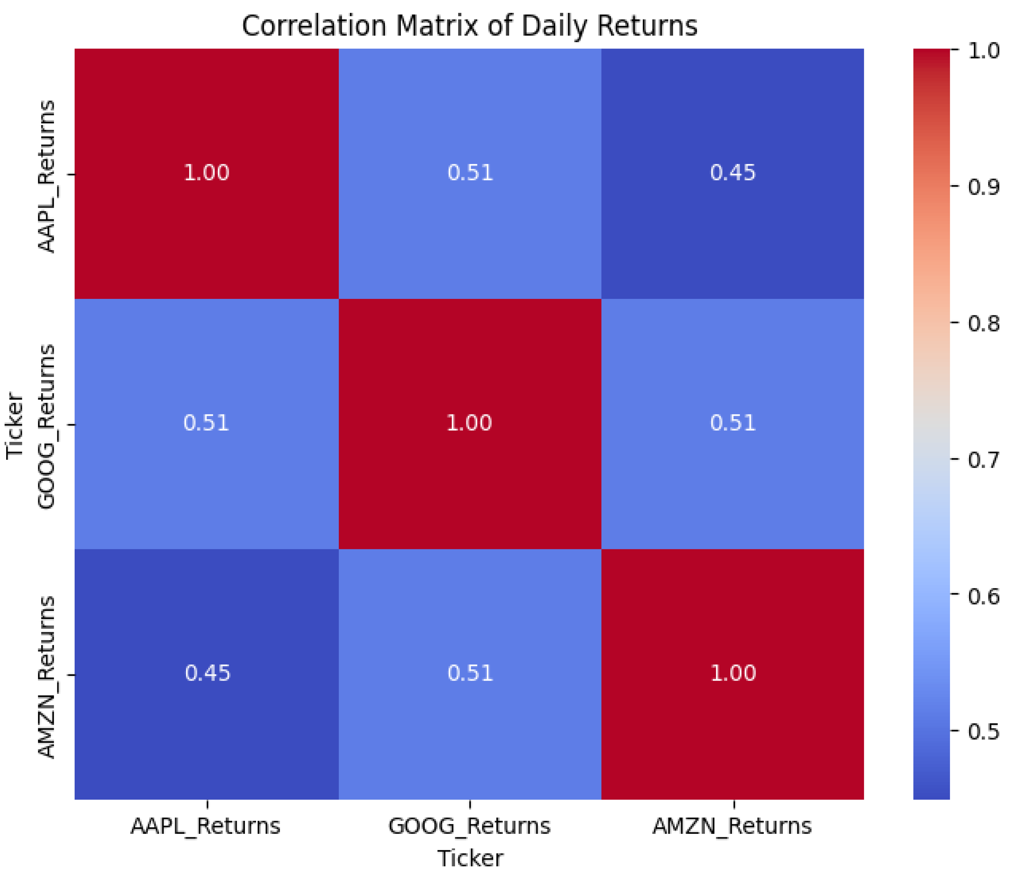
In order to investigate the interdependencies between the assets, I estimated the correlation matrix of the daily returns. In this way, I could analyze to what extent the stocks move together in times of calm market conditions and in times of market volatility. The findings indicated that, although the assets have a general correlation, the intensity of the correlation varies across various periods—most notably for the pre-COVID-19 market crash period.
I also compared the return distributions of both stocks. Histograms and KDE plots such as the ones shown above indicated that the data is not normally distributed and fat-tailed — a common property of financial returns that justifies the use of generative models like diffusion-based methods.
The first analysis furnished the foundation for the modeling stage and enabled the architectural choices that had been made during the model's design process.
Figure 1.
Daily returns of APPLE, GOOGLE and AMAZON.
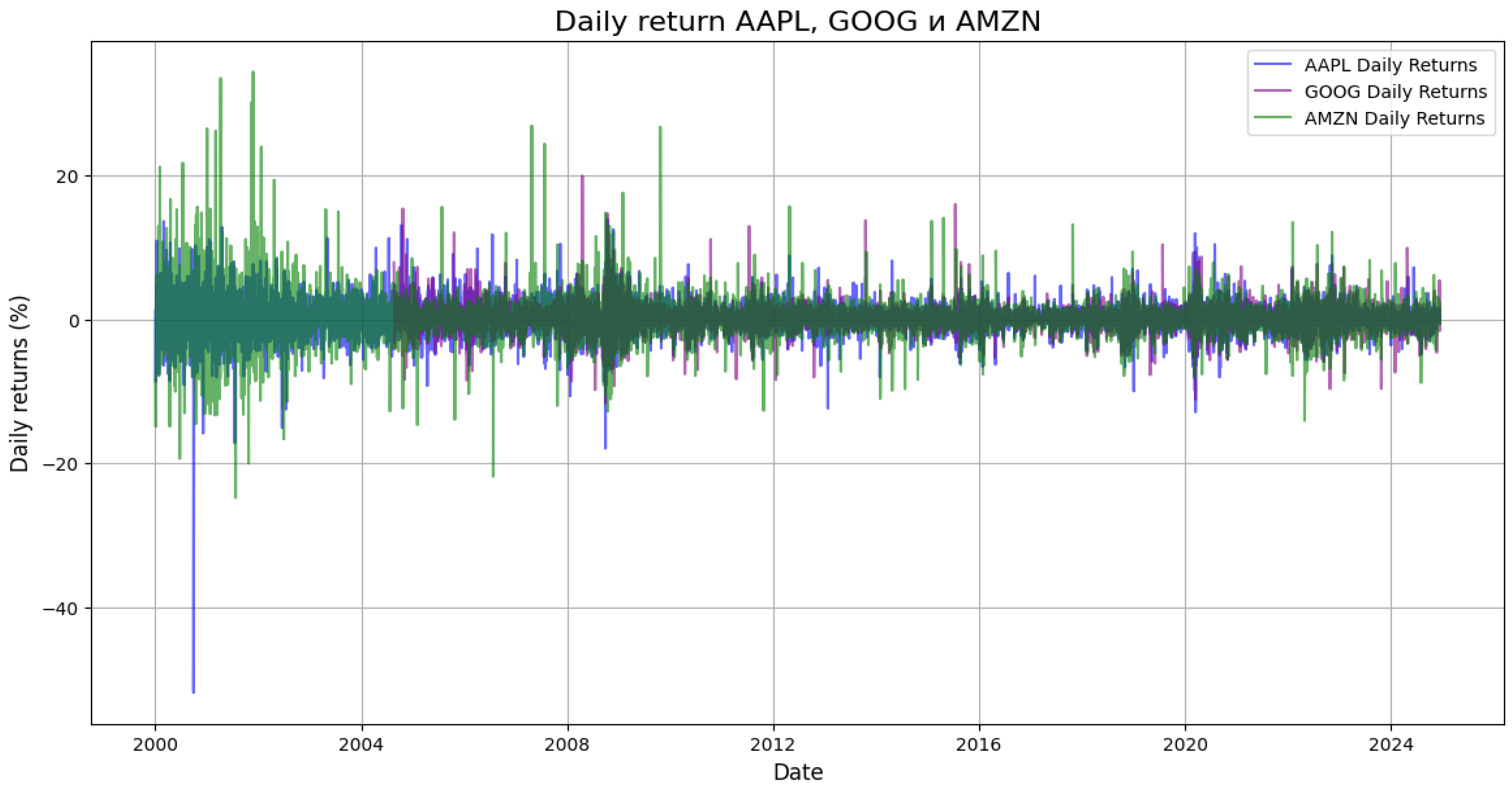
Figure 2.
Correlation Matrix of Daily Returns.
In order to better understand the data structure and identify the characteristics of asset behavior in different periods, I conducted an analysis of daily returns and correlations between AAPL, GOOG and AMZN stocks. The division into three key stages — before the pandemic, during COVID-19, and after — made it possible to track how the relationship between assets changed in the face of market instability.
Graphs of yields and correlations helped to visualize:
- periods of high volatility (for example, in 2020),
- dramatic increase in synchronicity between assets during the crisis,
- a return to a more fragmented dynamic after it.
This analysis confirmed that the market does not behave the same over time, and that the statistical properties of assets depend on the regime. Therefore, it was important to use a model that could account for instability, nonlinear dependencies, and the "thick tails" of the yield distribution. It is precisely these requirements that are met by the diffusion generative approach, on which the main model in this study is based.
Figure 3.
Returns APPLE, GOOGLE and AMAZON on COVID-19 period.
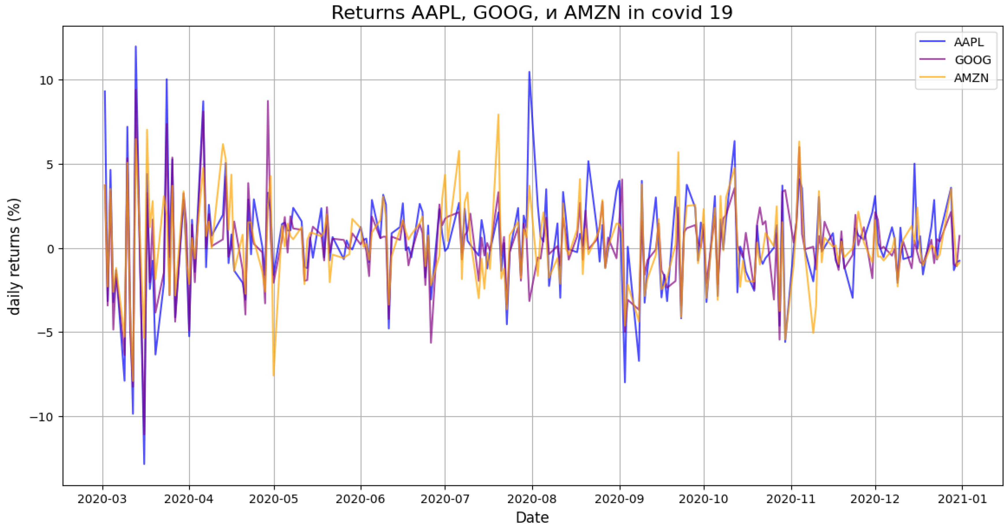
Figure 4.
Correlation matrix in COVID-19 period.
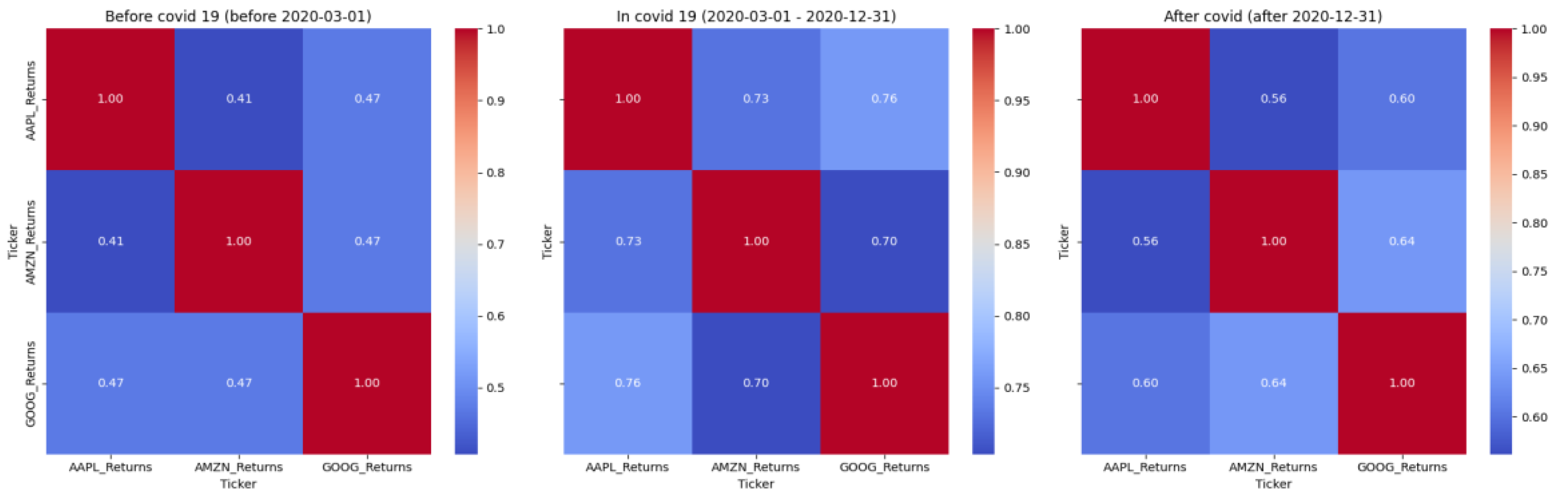
Figure 5.
Split on train and test.
4.5. Data Normalization
Yields from different companies behave differently - some are more volatile, others change smoothly. In order to avoid skewing towards "noisy" assets when training the model, I decided to bring the data to a single scale. Three different normalization methods were used for this.:
Z-score: ;
Min-Max scaling: ;
Logarithmic transformation: ;
4.6. Model Training
To test how well our diffusion-based model works, we trained it on daily returns that were standardized beforehand. The training ran for 300 full passes through the data (epochs), and we used a learning method (Adam optimizer) that adjusts weights step by step, based on how wrong the predictions are. Our goal was to reduce the difference between added noise and the noise predicted by the model, using a basic squared error approach.
Forward process(adding a noise):
Reverse process(reverse generation):
During the training, we used a specific schedule to control the amount of noise added at each step. When it was time to generate new samples, the model reversed this noise process step by step, creating data that should look similar to real returns. We also applied constraints to keep the generated values from going into extreme ranges.
To see how our model compares, we built and trained three other models:
- A simple multilayer network that tries to learn the data directly,
- A variational autoencoder (VAE) that learns a compressed version of the data and tries to reconstruct it,
- A generative adversarial network (GAN) that trains two models to compete — one generates data, and the other tries to detect if it’s real or not.
In addition to distributional metrics, we also evaluated how close the predicted values were to the real ones using traditional regression scores. Specifically, we used mean squared error (MSE) to measure the average prediction error, and R² to check how much of the variability in the target values the model was able to explain. These metrics are especially useful when comparing direct predictors such as MLP or VAE to our DDPM, even though the latter is not trained as a point estimator.
Mean Squared Error(MSE):
R-Squared(:
Our diffusion model showed stronger performance. It generated samples that were statistically closer to the real data, and the estimated tail risk was more accurate than the other methods.
4.7. Results
In this part of the research, we provide the result of CVaR calculation using a generative model of Denoising Diffusion Probabilistic Methods (DDPM). To compare, the model output was compared with two conventional methods: Historical Simulation and Monte Carlo Simulation. Due to the computational difficulty in handling the enormous S&P 500 data, typically beyond the capacity of normal computing, our research was limited to a representative sample of three of the most dominant stocks: Apple (AAPL), Amazon (AMZN), and Google (GOOGL). These firms were selected based on their high liquidity and significance to the index, thus offering a big enough foundation to assess model performance without lowering the generalizability of overall results.
Figure 6.
Predicted vs actual returns. The model closely follows real data and reflects major fluctuations, which supports its use for risk analysis.
Figure 6.
Predicted vs actual returns. The model closely follows real data and reflects major fluctuations, which supports its use for risk analysis.
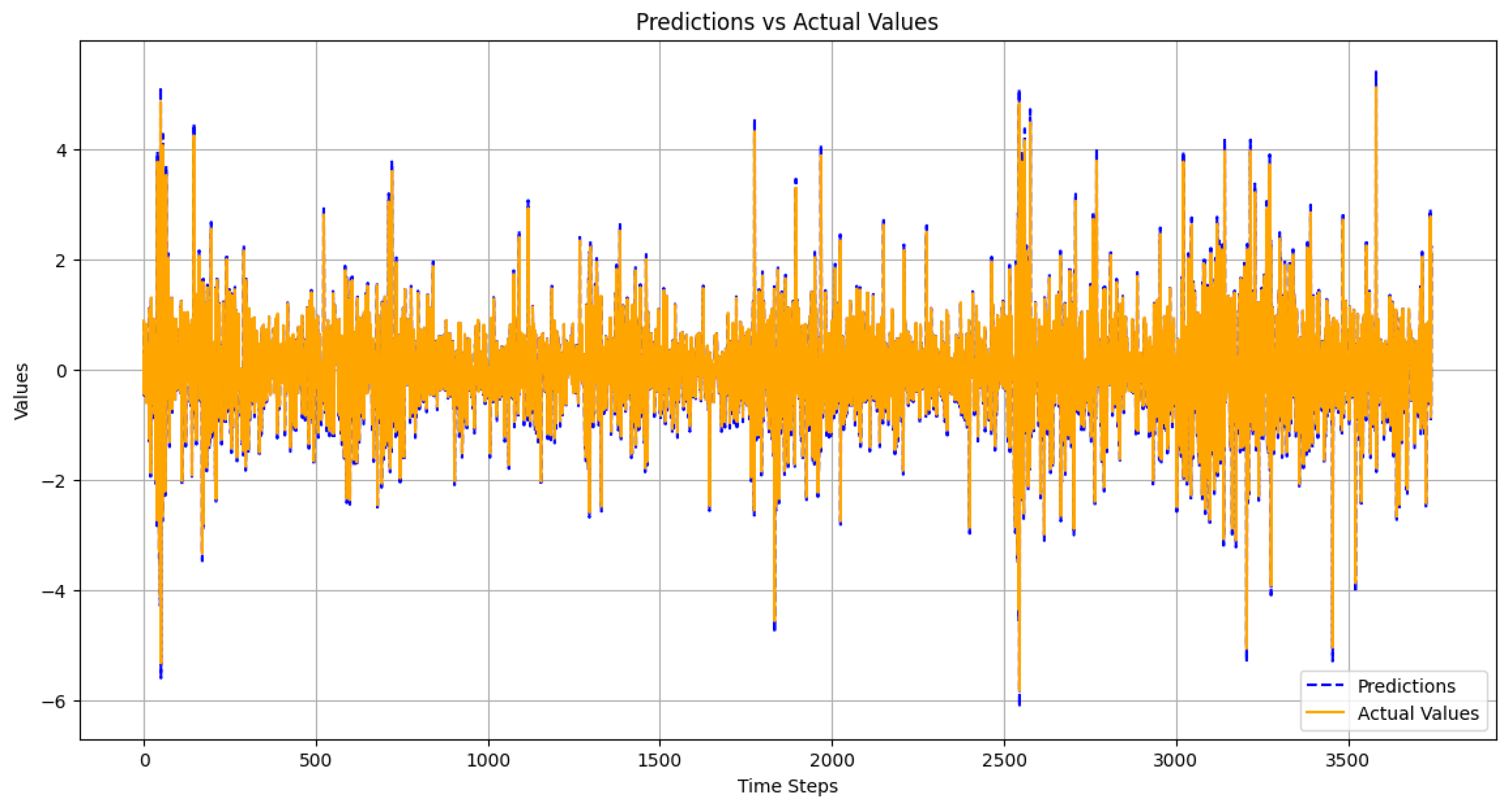
This plot contrasts forecasted values according to the diffusion model with true return history over time. From the chart, one can see that the forecasts run very close behind the actual movements for most of the series. The model captures both the overall trend and short-run fluctuations, even as it misses some of the more extreme spikes at times. Overall, this alignment suggests that the model is able to learn the underlying data structure and replicate it quite well, which is important for establishing risk in volatile situations.
The estimation was conducted on daily return data with focus on the 5% tail of the distribution. We can see from Table 1 that the CVaR as estimated by the DDPM model differs from the true test CVaR by only -0.20, while the conventional methods had higher positive deviations between 0.27 and 0.29. This indicates that the generative method provides a more precise and realistic estimation of the tail risk.
Besides the quantitative comparison of CVaR values, I also conducted an examination of the shape of the return distributions realized under each approach. This was done so that we would have some sense of how each approach handles large negative returns, a challenge which has a direct impact on CVaR estimation accuracy. The graph in Figure 1 illustrates the degree to which the distribution of the DDPM model aligns with the test data itself, particularly in the lower tail, where losses are more likely to be incurred. Yet, both Historical Simulation and Monte Carlo approaches seem to dampen the impact of the tail, which can result in loss underestimation. This visual discrepancy confirms the results above and illustrates the value of incorporating generative models in risk measurement.
Figure 7.
Comparison of return distributions and risk thresholds (VaR and CVaR at 5%) across three methods: Historical Simulation, Monte Carlo, and the proposed DDPM-based model. The DDPM distribution demonstrates closer alignment with the real test data in the lower tail region, indicating more accurate modeling of extreme losses.

To find the predictability of the model with Diffusion Denosing Probabilistic Models (DDPM), training data were 5-fold cross-validation tested. In every instance, the model showed low error rate and explanatory power in all folds. Mean Squared Error (MSE) was between 0.0009 and 0.0027, and the coefficient of determination (R²) was greater than 0.997 in all the folds. On average, the model estimated MSE to be 0.0016 and R² to be 0.9984, indicating that there was good fit between observed and predicted values and data structure was highly explanatory in nature.
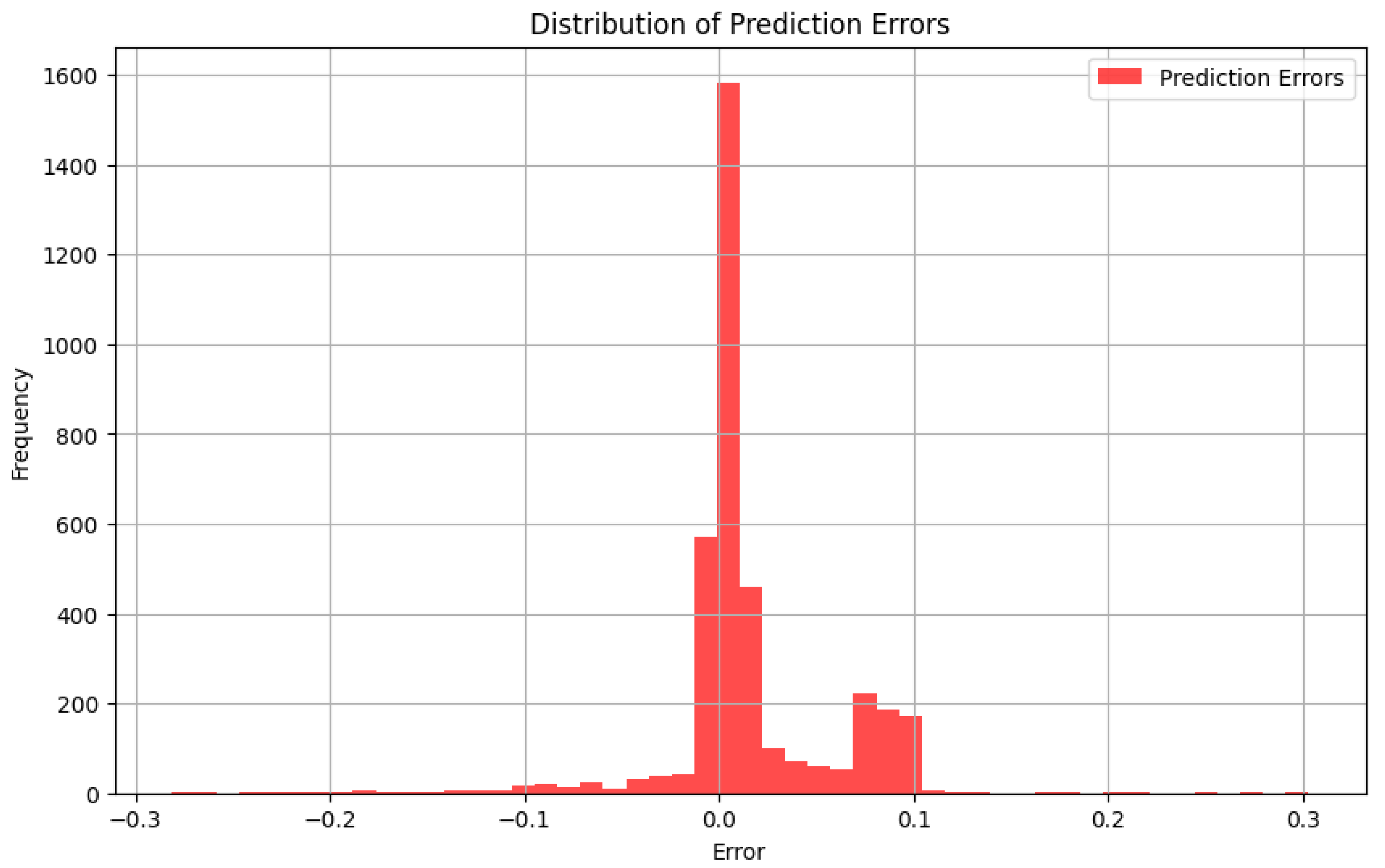
To better estimate the quality of predictions made by the DDPM model, we analyzed the distribution of prediction errors, which we have defined as the difference between the predicted and actual return values. A well-performing model should have errors concentrated around zero with low dispersion. The below histogram shows the distribution of prediction errors over the whole test set.
Figure 8.
Error histogram of predictions. The majority of the errors lie near zero, indicating that the model makes unprejudiced predictions with reasonably low variance.
Figure 8.
Error histogram of predictions. The majority of the errors lie near zero, indicating that the model makes unprejudiced predictions with reasonably low variance.
To check the model's ability to generalize, I trained the model on return data for Apple (AAPL) and Amazon (AMZN) and tested it on an unseen stock, namely Google (GOOGL). The aim was to check if the model could recognize and learn about a new asset that it wasn't exposed to during training. The predicted returns on GOOGL were checked against the actual returns for the same period of time. Although the asset was not in the training set, the model had predictions that followed the actual data closely enough with a very low mean squared error and very high R² score. That indicates the model would be able to generalize patterns learned from AAPL and AMZN to another asset with similar market action.
Figure 9.
Predicted vs actual returns for GOOGL. The model was trained only on AAPL and AMZN. Despite having no prior exposure to GOOGL, the predictions track the actual values closely, demonstrating the model's ability to generalize across similar financial assets.
Figure 9.
Predicted vs actual returns for GOOGL. The model was trained only on AAPL and AMZN. Despite having no prior exposure to GOOGL, the predictions track the actual values closely, demonstrating the model's ability to generalize across similar financial assets.
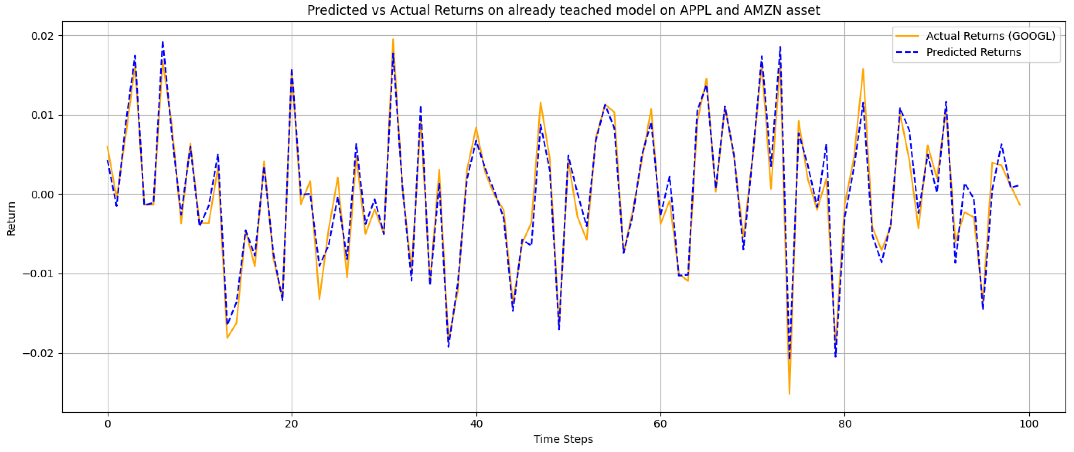
Figure 10.
Illustration of the DDPM training pipeline. The original image is gradually corrupted with noise through multiple stages, producing an intermediate noisy sample ztz_tzt. A U-Net model is then trained to reverse this process by predicting the clean signal or the noise component, enabling recovery of the original image through denoising.

5. Conclusion
In this work, I explored the use of a denoising diffusion probabilistic model (DDPM) to estimate Conditional Value-at-Risk (CVaR) and compare it with other more traditional approaches such as Historical Simulation and Monte Carlo. The experiments showed that the DDPM model was capable of generating realistic return distributions with improved tail capture of financial loss compared to the baseline models. Especially, generative model estimates of CVaR were always nearest to respective test data values.
Cross-validation outputs printed out low, consistent prediction errors across all of the folds, which is suggestive of the fact that the model was not susceptible to overfitting and generalized well to train data. Secondly, model evaluation using another, unseen asset (GOOGL) ensured that it had been successful at generalizing learned pattern to other new financial assets, at least in similar market context.
From the findings, I recommend utilizing generative models like DDPM in risk estimation where traditional methods are constrained, specifically when modeling tail risk. This is despite the promising findings since future work can be focused on improving calibration of models, incorporating time dependencies, or measuring performance across a broad asset universe and during economic stress.
Acknowledgements
This project took time, effort, and quite a few moments of doubt — and I couldn’t have done it alone. I want to thank my advisor for helping me stay focused and for giving practical, no-nonsense feedback throughout the process. I’m also grateful to my family for quietly supporting me in the background — even when I was too busy to notice. A few friends kept me sane and on track when things got overwhelming, and for that, I owe them more than just thanks. Finally, I’ve learned a lot more than I expected while working on this — about the topic, and about how I work when things get difficult.
List of Abbreviations
| CVaR | Conditional Value-at-Risk |
| VaR | Value-at-Risk |
| DDPM | Denoising Diffusion Probabilistic Model |
| MSE | Mean Squared Error |
| R² | Coefficient of Determination (R-squared) |
| GRU | Gated Recurrent Unit |
| MLP | Multilayer Perceptron |
| VAE | Variational Autoencoder |
| GAN | Generative Adversarial Network |
| S&P 500 | Standard & Poor’s 500 Index |
| GOOGL | Alphabet Inc. (Google stock ticker) |
| AAPL | Apple Inc. stock ticker |
| AMZN | Amazon.com Inc. stock ticker |
| MSFT | Microsoft Corporation stock ticker |
| TimeGrad | Time Series adaptation of DDPM |
References
- Wang, M., Liu, Y., & Wang, H. (2024). Expected shortfall forecasting using quantile regression and generative adversarial networks. Financial Innovation, 10(1), 1–20. [CrossRef]
- Sicks, R., Buch, R., & Kräussl, R. (2021). Estimating the Value-at-Risk by Temporal VAE. arXiv preprint arXiv:2112.01896. https://doi.org/10.48550/arXiv.2112.01896. arXiv:2112.01896. [CrossRef]
- Buch, R., Sicks, R., & Kräussl, R. (2023). Estimating the Value-at-Risk by Temporal VAE. Risks, 11(5), 79. [CrossRef]
- Fatouros, G., Giannopoulos, G., & Kalyvitis, S. (2022). DeepVaR: A framework for portfolio risk assessment leveraging probabilistic deep neural networks. Digital Finance, 5, 135–160. [CrossRef]
- Ho, J., Jain, A., & Abbeel, P. (2020). Denoising diffusion probabilistic models. arXiv preprint arXiv:2006.11239. [CrossRef]
- Rasul, K., Becker, S., Dinh, L., Schölkopf, B., & Mohamed, S. (2021). Autoregressive denoising diffusion models for multivariate probabilistic time series forecasting. arXiv preprint arXiv:2101.12072. arXiv:2101.12072. [CrossRef]
- Bond-Taylor, S., Leach, A., Long, Y., & Willcocks, C. G. (2021). Deep generative modelling: A comparative review of VAEs, GANs, normalizing flows, energy-based and autoregressive models. IEEE Transactions on Pattern Analysis and Machine Intelligence, 44(11), 7327–7347. [CrossRef]
- Tobjork, D. (2021). Value at risk estimation with generative adversarial networks (Master’s thesis). Lund University. https://lup.lub.lu.se/luur/download?func=downloadFile&recordOId=9042741&fileOId=9057935n with generative adversarial networks (Master’s thesis). Lund University. https://lup.lub.lu.se/luur/download?
- Acerbi, C., & Szekely, B. (2014). Back-testing expected shortfall. Risk, 27(11), 76–81.https://www.msci.com/documents/10199/22aa9922-f874-4060-b77a-0f0e267a489b.
- Cont, R. (2001). Empirical properties of asset returns: stylized facts and statistical issues. Quantitative Finance, 1(2), 223–236. [CrossRef]

Table 1.
Comparison of VaR and CVaR (5%) estimates across four methods: Historical Simulation, Monte Carlo, DDPM-generated values, and actual test results. The last column shows the deviation of each method’s CVaR from the real CVaR.
Table 1.
Comparison of VaR and CVaR (5%) estimates across four methods: Historical Simulation, Monte Carlo, DDPM-generated values, and actual test results. The last column shows the deviation of each method’s CVaR from the real CVaR.
| Method | VaR(5%) | CVaR(5%) | CVaR vs Real |
| Historical | -1.652590912772053 | -2.068221685641743 | 0.274340230778588 |
| Monte Carlo | -1.632568150548533 | -2.0458910638857457 | 0.296670852534585 |
| DDPM Generated | -2.1391024259601 | -2.542586058060833 | 0.200024141640501 |
| Real | -1.913492775354081 | -2.3425619164203315 |
Table 2.
Results from 5-fold cross-validation. The model showed stable performance with low error and consistently high R², which suggests it generalizes well to unseen data.
Table 2.
Results from 5-fold cross-validation. The model showed stable performance with low error and consistently high R², which suggests it generalizes well to unseen data.
| Fold | MSE | |
| 1 | 0.00272 | 0.9972 |
| 2 | 0.001399 | 0.9984 |
| 3 | 0.001361 | 0.9986 |
| 4 | 0.001596 | 0.9986 |
| 5 | 0.000906 | 0.9991 |
Disclaimer/Publisher’s Note: The statements, opinions and data contained in all publications are solely those of the individual author(s) and contributor(s) and not of MDPI and/or the editor(s). MDPI and/or the editor(s) disclaim responsibility for any injury to people or property resulting from any ideas, methods, instructions or products referred to in the content. |
© 2025 by the authors. Licensee MDPI, Basel, Switzerland. This article is an open access article distributed under the terms and conditions of the Creative Commons Attribution (CC BY) license (http://creativecommons.org/licenses/by/4.0/).
Copyright: This open access article is published under a Creative Commons CC BY 4.0 license, which permit the free download, distribution, and reuse, provided that the author and preprint are cited in any reuse.


