
Submitted:
18 December 2024
Posted:
19 December 2024
You are already at the latest version
Abstract
The reduction of mass and surface of antennas and scattering structures is an important task in designing electromagnetic devices. To solve this task, we present a novel algorithm based on the optimal current grid approximation (OCGA) for generating sparse scattering structures and evaluating their effectiveness. The main contributions of the work include analyzing the performance of the OCGA and its modifications in generating sparse antennas, as well as demonstrating the effectiveness of the algorithm in generating sparse scattering structures using a scattering plate as an example. To validate the accuracy of the algorithm, we compared the scattering properties of the obtained sparse scattering structures. The results show that the algorithm worked accurately and effectively in generating sparse scattering structures while reducing their mass and surface.
Keywords:
sparse antennas
; sparse scatterer
; optimal current grid approximation
; method of moments
1. Introduction
Antennas and scattering structures are widely used in various fields, from civil [1,2,3,4,5] to military [6,7,8,9,10]. With the continuous advancement of science, the demand for producing compact antennas and scatterers with intelligent designs is increasing [11,12,13,14]. Designing those structures to achieve required properties while maintaining low production costs necessitates high-accuracy simulation software with low computational costs. Simulating structures significantly reduces production costs, allowing for the assessment and optimization of structural properties before manufacturing. Additionally, it helps avoid technical errors during production [15]. Thus, simulation becomes an essential part of the design process for antennas and scattering structures [16,17]. However, accurate modeling may require intensive computations, especially when analyzing complex structures. In the meantime, the proper choice of numerical methods for modeling can significantly impact the cost and efficiency of the design process.
One of the common methods for analyzing antenna and scatterer structures is the method of moments (MoM) [18,19,20,21,22]. MoM is based on transforming the integral equations of the electric field into a system of linear algebraic equations, and then the current distribution in the structure is determined by inverting the impedance matrix [23,24]. MoM is considered to have a simple algorithm and low computational costs compared to other methods, while allowing for acceptable simulation results. Based on MoM, many new approaches to modeling antennas and scatterers have been developed [25,26,27,28,29]. One prominent method is the surface approximation of structures using wire grid (WG). This approach simplifies the surface shape, making the implementation of modeling in source code easier. Multiple studies on modeling antenna and scattering structures have been conducted taking advantage from this approach (WG based on MoM) [30,31,32,33,34].
The reduction of antenna mass is an important factor in many engineering fields [35,36]. Low mass and compact size not only reduce transportation costs (for example, into space [37,38]), but also simplify installation and maintenance, and can minimize negative environmental impacts on the structure (for instance, wind and rain).
Similarly, in the field of interferometric synthetic aperture radar (InSAR), corner reflectors (CRs) are a typical example of scattering structures [39,40,41,42]. These structures are prominent because of their ease of fabrication and significant scattering capabilities over a wide range for incident plane waves. However, a clear disadvantage is that the size of CRs is often quite large (for example, a trihedral CR can have edge lengths of up to 2.5 m [43]). In addition to their bulky size, the weight of these structures is also relatively high, mainly due to the use of conductive metal materials. Therefore, reducing the mass of these structures to facilitate transportation, installation, and maintenance is an important issue that needs to be solved.
Several methods have emerged to reduce the weight and size of these structures. One example is using silver-coated textiles [44]; however, a disadvantage of this method is that the conductive material is susceptible to environmental factors. In addition, the silver-coated technology is complex and expensive. Another method is the use of structures with a perforated plate [45]. Although this method significantly reduces the weight of the entire structure and improves drainage of accumulated rainwater [46], the perforation process complicates manufacturing and increases costs [47]. Moreover, perforating can often cause surface deformation [43]. Therefore, there is a need to develop new methods to reduce the weight of such structures.
Recently, there has been developed a technique for reducing antenna mass and surface using OCGA based on MoM and WG. This technique allows for easy implementation of algorithms to create sparse structures by removing wires with low current magnitudes from the structure. The application of OCGA not only significantly reduces the mass and surface of the structures but also decreases computational costs, including calculation time and the necessary computer memory [38]. When it is necessary to reduce the mass and surface of scattering devices, using OCGA to design sparse scatterer structures becomes truly essential. However, the biggest difference between antenna and scattering structures is the characteristics of the excitation source. In antennas, the source is typically fixed [6], while in scattering devices, the source depends on many parameters of the incident wave, for example, direction, polarization, wave front (spherical, plane, etc.) [48,49]. Therefore, applying OCGA to scattering structure presents more challenges.
CR structures are composed of flat metal plates with various shapes [50,51]. Therefore, reducing the mass and surface of rectangular flat scattering plates will be considered a preliminary study to apply the OCGA algorithm to more complex scattering structures in the future. In addition, the synthesis and review of the results related to the reduction of antenna mass and surface based on OCGA will provide more insight into the effectiveness of this algorithm. This will facilitate the application of OCGA to reduce the mass and surface of scattering structures. Therefore, the aim of this paper is to present the results of sparse antennas generation summarized from previous studies, develop an algorithm for generating sparse scattering structures based on OCGA, and discuss the obtained results.
This paper is organized as follows. Section II presents a comprehensive review of approaches for reducing mass and surface of various antenna structures using the OCGA. Section III presents the results of validating scattering characteristics for the plate scatterer structure, obtained using MoM with pulse basis function (PBF) based on WG. Section IV introduces an algorithm to sparse the scattering structure when it is excited by an incident wave at a specific direction. Section V presents another algorithm to generate sparse scattering structures when the excitation direction of the incident wave changes. Section V analyzes the sparse structures when the specific excitation region of the incident wave is unknown, and Section VI analyzes when the specific excitation region of the incident wave is known. Section VII summarizes and discusses the results obtained and highlights the points to consider for future studies, followed by conclusions in Section VIII.
2. Review of Sparse Antennas
The MoM is widely used for modeling different antenna designs with low computational cost and optimizing their designs to meet specific requirements. A review of the antenna modeling history using the MoM and the potential of using WG to approximate the solid metallic surface of different antenna types is presented in [38]. To further reduce the antenna mass, surface and computational cost, sparsifying WG antenna structure by using OCGA was firstly proposed in [38]. The OCGA works based on obtaining the current distribution in WG structure. After this, the current magnitudes in each wire are normalized by their average or maximum value. Then all wires with current magnitudes less than a certain threshold are eliminated since their contribution to the radiation is negligible. This threshold is called the grid element elimination tolerance (GEET) and can be adjusted according to each specific requirement. The result is a sparse WG structure that includes only wires with large currents. Compared with the original WG structure, the sparse WG structure has lower antenna mass and surface as well as its modeling cost.
To generate sparse WG structures using OCGA, it is necessary to accurately approximate the solid metal surface of the antenna using WG. Many recommendations have been proposed in the past for approximating metal surfaces using WG. However, they are not complete and are not suitable for creating an original WG structure to which OCGA can be applied to create a sparse structure. The suitability and inadequacy of the previous recommendations are presented in detail in [52]. Therefore, new recommendations were proposed in [52] for approximating the solid surface of horn structures using WG, which can be used as an original structure for applying OCGA to create a sparse structure. An approximate comparison of antenna surface using WG with different cell types such as square and trapezoidal was carried out in [53]. In [54], the authors compared antenna surface approximation using WG and OCGA to create sparse structures in different CAD systems such as TUSUR.EMC [55], MMANA-GAL [56], and 4NEC2 [57]. In addition, an optimization method based on OCGA was proposed in [58] to generate sparse WG structures that meet the given criteria. The algorithmic details of this optimization method were presented and software with a user-friendly interface was developed based on this method.
However, the WG structure obtained after OCGA encounters difficulties in fabricating unprinted antennas due to the presence of wires not connected to the structure (free wires). To overcome these difficulties, a modification of OCGA to create a sparse WG structure with connected current paths was proposed in [38]. This modified approach is referred to as “Connecting” OCGA (COCGA), and its main idea is to recover radial wires to create a current path between the free wires and the structure, since for radial structures these wires usually carry large currents. The algorithm details of the OCGA and COCGA approaches were presented in details in [38]. The OCGA and COCGA approaches have been applied to a reflector antenna (5.1-5.9 GHz), a horn antenna at 8 GHz, perforated X-band horn antenna (8-12 GHz), and a conical horn antenna at 8 GHz. A comparative analysis of the sparse structures obtained after applying OCGA and COCGA to these types of antennas was presented in [59] in detail. The results of the comparative analysis show that COCGA generally results in antenna characteristics closer to the original structure, demonstrating higher accuracy in preserving the original characteristics, while OCGA also demonstrates the possibility of reducing the antenna mass and surface as well as the time and memory requirements for subsequent modeling. In addition, [60] presented details on the classification of hidden antenna types and the possibility of using sparse WG structures to design hidden antennas that meet specific requirements.
Since the current distribution on the obtained WG structure is different at different frequencies in the operating frequency range, the effect of frequency selection on the obtained sparse structure after OCGA and COCGA application on the horn antenna X-band (8-12 GHz) was analyzed in [61]. The analysis results show that the sparse structures obtained based on the current distribution at the lowest frequency in the operating frequency range provide antenna characteristics closer to those of the original antenna and less dependent on the GEET value, compared to the other structures. In addition, at the highest frequency in the operating frequency range, the sparse structures obtained after COCGA provide results with minimal differences compared to the original structure.
The sparse structure obtained after COCGA has antenna characteristics close to those obtained for the original structure. However, it recovers a large number of radial wires to maintain the current paths in the structure and its continuity, which leads to a nonoptimal reduction in mass and simulation cost. Therefore, OCGA modifications were proposed in [62] to create a sparse WG structure with all wires interconnected. These approaches were referred to as “Eliminating” OCGA (EOCGA) and “Near-Connecting” OCGA (NCOCGA). To provide a current path in the sparse WG structure, EOCGA eliminates all free wires in the sparse WG structure obtained after OCGA, while NCOCGA restores only those wires that are necessary to connect these free wires to the structure. The algorithms of these approaches were discussed in detail, and their performance was verified on different types of antennas.
However, the algorithms of these approaches were based on the geometric position of the wires in the grid, which limits their accuracy. Furthermore, they are only applicable to radial WG designs such as antenna reflectors and conical horn antennas. Therefore, new algorithms were proposed in [63] to improve the OCGA approach and its modifications, which aim to use the start and end coordinates of the wires in combination with an algorithm for finding free wires and determining the shortest path to connect them. The results obtained after applying the modernized algorithms were compared with the results of the previous algorithm. The comparison results showed that these new algorithms had higher accuracy, efficiency, flexibility, and could be applied to many different types of WG structures.
The OCGA, EOCGA, and NCOGA with the modernized algorithms have been applied and shown to be effective in creating sparse structures on various types of antennas operating at various frequency bands. A series of prototypes, original WG and sparse WG structures obtained after applying various approaches on various types of antennas are presented in Table 1. The improvements in antenna mass and surface, memory and time cost in subsequent modeling for various sparse structures were obtained after applying different approaches to different types of antennas compiled from different works and presented in Table 2. Moreover, Table 2 also summarizes the maximum differences in characteristics of these sparse antennas compared to the original antenna in the operating frequency range. Then comparative analyses were performed to analyze the effect of frequency selection on the sparse structure generated after applying different approaches [61,64,65,66,67,68,69].
After the comparative analysis, these works provide conclusions and recommendations about the following:
- The approach that provides better reduction in antenna mass, surface and cost for subsequent modeling (approach for reduction);
- The approach that provides the best antenna characteristics (approach for characteristics);
- The frequency at which the sparse structure is created is based on the current distribution at the frequency that has the best characteristics (current distribution for sparse structure);
- The frequency at which the antenna characteristics of the sparse structure are obtained least dependent on the GEET value (frequency for characteristics).
The sparse WG structures presented in Table 1 demonstrate the accuracy of various approaches. OCGA excluded the wires with normalized smaller current magnitudes than a given GEET value and obtained the corresponding sparse WG structures. However, it can be seen that some free wires appear in the sparse structures after OCGA. Therefore, EOCGA eliminated them while NCOCGA recovered the necessary wires to connect them to the WG structure. The sparse structures obtained after EOCGA and NCOCGA had no free wires. This confirms the correct performance of the modernized algorithms, since they can be applied to various antenna structures. The results summarized in Table 3 show that the greatest value of antenna mass and surface reduction and simulation cost is usually obtained after OCGA and EOCGA, and the smallest value of the maximum antenna characteristic difference when compared with the results obtained for the original structure is usually obtained for the sparse structure after NCOCGA. Comparing the sparse structures obtained based on the current distribution obtained at different frequencies, it can be noticed that virtually all works recommend that the sparse structures are generated based on the current distribution at the lowest or center frequency in the operating frequency range. Moreover, when comparing the antenna characteristics obtained at different frequencies for sparse structures, the antenna characteristics obtained at the highest frequency in the operating frequency range are stable and less dependent on the GEET value than at other frequencies.
All the results obtained after applying OCGA and its modifications on different antenna structures operating at different frequencies demonstrate the effectiveness of these approaches in creating sparse structures. The sparse antenna structures have lower mass, surface and modeling cost than the original structure, while the antenna characteristics are maintained. Sparse antenna structures can be used to fulfill various requirements, such as in IoT devices or space applications where there are severe specifications on antenna mass and size. In addition, they can be used in applications that require hidden antennas so as not to affect the overall landscape.
3. Verification of the Modeling Results for Scattering Plate Using MoM Based on WG Model
Section II demonstrated the effectiveness of using OCGA and its modifications in generating sparse antenna structures. Therefore, it is reasonable to apply this approach to develop algorithms for generating sparse scattering structures. However, first, to verify the accuracy of using MoM with PBF based on WG in scatterer analysis, we verify the scattering field results obtained for a flat plate scattering structure.
The shape of the rectangular perfect electrically conductive plate scatterer from [70] is illustrated in Figure 1a. The plate is positioned in the xOz plane and is orthogonal to the Oy-axis. The origin of the coordinate system coincides with the center of the plate. The structure has a length of H=3λ and a width of W=2λ. Figure 1b depicts the plate from Figure 1a, approximated using a WG in this study. The WG structure consists of the same square cells: 30 cells along the H edge and 20 cells along the W edge, while Δ represents the edge length of all the WG cells, which is equal to the length of each cell wire. Each of the four wires forming the WG cells is represented by a single segment. This approach simplifies the construction of the structure and complies with the recommendations that no basis function passes through the intersection points of the segments.
In the process of modeling the rectangular plate scatterer, the segment length (Δ=λ/10) and the wire radius (a=Δ/2π) were calculated based on the findings of previous publications. Specifically, at the excitation frequency f=300 MHz, the dimensions of the plate were H=3 m, W=2 m, Δ=0.1 m, and a=0.016 m. A plane wave with θ-polarization was utilized for excitation at the incident angles θinc, ϕinc. When calculating the backscattering cross section (BSCS), the scattered field was considered at the angles θscat=θinc, ϕscat=ϕinc.
In this work, the BSCS of the structure was calculated using MoM with PBF based on WG and compared with numerical simulation results using MoM with piecewise-sinusoidal (PWS) basis functions, as well as with experimental results from [70] (Figure 2). The obtained results coincided well with each other. In fact, the BSCS results using MoM with PBF based on WG matched even more closely with the measured results than those obtained with MoM using PWS, particularly when the direction of the incident wave changes in the xOy plane. Although there were differences in the results at the side lobes, the results in the main lobe of the BSCS generally matched well. Additionally, when the incident wave was perpendicular to the surface of the plate, the scattered field reached its maximum; specifically, the BSCS magnitude at θ=90°, φ=90° were 26.8 dBsm (MoM with PBF based on WG) and 26.25 dBsm (experimentally and MoM with PWS). Note that the width of the main lobe (–3 dBsm from the maximum BSCS level) obtained in the xOy plane (12°) was larger than that in the yOz plane (8°), which was consistent with the fact that the width of the plate (W=2 m) was smaller than its length (H=3 m). These findings demonstrate the accuracy of using MoM-based WG with PBF for analyzing scattering plate structures.
4. The OCGA Approach for Creating Sparse Scatterers
The results obtained in Section III have verified the accuracy of approximating the perfect conducting flat plate using the WG structure. However, as mentioned above, it is not necessary to use all the wires of the grid to simulate the plate. Therefore, in this section, we present an OCGA-based approach for the initial WG scattering structure when the incident wave is at a fixed direction, aiming to achieve a sparse WG structure.
Since OCGA is based on the characteristics of surface current, it is essential to analyze the current distribution in the structure when it is excited by a plane wave. In this section, we assume that the incident wave has θ-polarization perpendicular to the plate, which means that the horizontal wires are completely unaffected by the incident plane wave. As a result, the current that appears on the horizontal wires is very small compared to that on the vertical wires. Figure 3 presents the magnitude of the obtained current distribution (|I|) at the left vertical edge (AB) and along the central vertical line (EF) of the plate. It is observed that |I| along the plate at the edge (=1.23 mA) reaches a higher value compared to that at the center line of the plate (=0.68 mA).
According to electromagnetic theory, the tangential component of an electric field must be continuous across the boundary between two media (in this case, the surface of the plate). However, the sudden changes in geometric shape at the edges of the plate caused significant variations in the electromagnetic field. Specifically, in the central region of the plate, the electromagnetic field is distributed uniformly across the surface, while at the edges, the electric field was more intensely excited. This phenomenon leads to high accumulation of electric charge at the edges, resulting in high current at these locations (edges AB and CD). In contrast, the current distribution obtained in the central region of the plate surface is lower.
We developed the OCGA algorithm to create a sparse scatterer structure (Figure 4). After applying MoM with PBF based on WG to the plate, |I| was obtained for all wire segments. The obtained |I| was then normalized by its maximum value (|I|max). Subsequently, the normalized current results (Inor) were compared with GEET. Segments with Inor values smaller than GEET were removed from the initial WG structure. As a result, the obtained sparse structure consists only of segments with Inor values greater than GEET. The indices of the segments in the sparse structure were stored in a matrix denoted as Ms, which has the size of 1×Ns where Ns is the total number of segments in the sparse structure.
Then, we calculated the impedance matrix (Zs) and excitation vector (vs) for the sparse scatterer to determine the scattering characteristics of the structure. There are two approaches to achieve this.
The first approach involves recalculating the elements of Zs and vs directly using MoM with PBF for the sparse structure. This approach is easy to implement in code. However, as mentioned earlier, actual scattering structures are electrically large (much larger than λ), which means that their modeling using WG requires a significant number of segments (N) (potentially reaching tens of thousands). Even after sparsing the structure, there are still quite a few segments to consider. Therefore, recalculating Zs and vs using this approach significantly increases the computational cost.
The second approach leverages a significant advantage related to the formation of the initial impedance matrix (Z) using the MoM with PBF. When an i-th segment is removed from the structure, it is sufficient to eliminate the corresponding i-th row and i-th column in matrix Z. In other words, the existence of each individual segment is independent of the others, which contrasts with the use of basis functions constructed from points along the wire (e.g., triangular functions). Therefore, this approach is considered more optimal in this context. Furthermore, this approach not only accelerates Zs computation but also facilitates the rapid identification of the vs element by removing the i-th elements (corresponding to the index i of the removed segment) from v (the excitation vector for the initial WG). As a result, the computational cost of analyzing the scattering characteristics of the sparse structure is significantly reduced.
Next, we analyzed the results of using OCGA to sparse the considered WG structure. In previous publications [71], [72], the scattering characteristics of the rectangular plate, as represented by the radar cross section (RCS), are typically examined when the incident wave is directed orthogonally to the plate (θinc=ϕinc=90°). Therefore, in this section, we first investigated the variation of the RCS maximum magnitude (RCSmax) (when θscat=ϕscat=90°) for the plate when the GEET value changed (Figure 5).
From Figure 5, it can be observed that when GEET is set to 0–34%, the RCSmax value remains largely unchanged. This is because, in addition to the horizontal segments, which does not contribute to the scattering field, the |I| of the vertical segments is generally greater than GEET (exceeding 34% of |I|max). Specifically, as seen in Figure 5, |I|min on segment EF is 0.44 mA, which is still greater than approximately 34% of |I|max on segment AB (1.23×0.34=0.41 mA).
When GEET increases to 34-55%, RCSmax decreases sharply. This can be explained by the fact that |I| on the vertical wires in the middle of the plate is smaller than the GEET value and leads to the removal of the wires. Furthermore, from Figure 5, it can be noted that |I| of the vertical wires in the middle of the plate is approximately equal, so even a slight increase in GEET within the range of 34-55% results in the removal of a significant number of vertical segments in that region. Unlike the case when GEET=0–34%, the removal of a large number of horizontal wires does not affect the scattering properties. However, the sudden decrease in the number of mid-plate segments (where |I| is not small) in this case leads to a sharp decrease in the scattering field, resulting in a rapid decrease in RCSmax in this range (Figure 5).
When GEET reaches 45%, RCSmax decreases significantly (down to 120 m²) and then increases again when GEET is at 46% (up to 240 m²). This phenomenon is not yet fully understood and may require the consideration of the phase of the removed segments rather than just comparison of the absolute values of current intensity; this will be made clear in future studies. When GEET is set to 56-100%, RCSmax drops to a very low value. This is because most of the segments in the middle of the plate have been removed, leaving only a few segments at the edges. Although the |I| in the remaining segments at the edges is large, the number of those segments is clearly insufficient to generate such substantial a scattering field as the field that is contributed by the segments in the middle of the plate.
From the above observations, it is clear that the number of wires removed from the WG structure depends on the GEET value: as the GEET value increases, the number of wires removed also increases. This directly impacts the mass and surface of the structure as well as the computational cost required for modeling the scatterer, such as the time and memory needed for subsequent simulations. According to [38], the time cost to solve a linear algebraic system of N order (using Gaussian elimination) scales with the cube of its order, O(N³); and the memory cost is O(N²). Consequently, the reduction in scatterer volume is proportional to N/Ns, while the time reduces as (N/Ns)3 and the memory requirement decreases as (N/Ns)2 where N is the total number segments of the WG structure and Ns – of sparse structure.
The dependence of the reduction in scatterer mass and surface, as well as the time and memory required for subsequent simulations, on GEET is illustrated in Figure 6. As noted, when GEET is very small (1%), the horizontal wires are removed from the structure. Meanwhile, the numbers of horizontal and vertical wires are nearly equal; thus, horizontal wire removal results in approximately a 2-time reduction in the mass and surface of the plate, which corresponds to about 8-time decrease in simulation time and 4-time reduction in memory usage. When GEET increases to 34%, these reductions remain constant, as previously mentioned (the vertical wires are largely retained).
When GEET is in the range of 34-55%, these reduction values decrease more rapidly because of the removal of many vertical segments in the middle of the plate. For GEET>55%, the reduction values still increase but not as rapidly, as the increase in GEET can only eliminate a certain number of vertical segments located at the edges of the plate.
However, as previously mentioned, changes in the number of wires in the WG structure directly affect the scattering characteristics of the structure. Therefore, this factor must be carefully analyzed before implementing sparse scatterers in production. Although we have broadly outlined the characteristics and variations of the scattering field as GEET changes, the analysis thus far has focused only on RCSmax. Consequently, we will next analyze the RCS and BSCS of the sparse structure at various GEET values.
Specifically, we selected the GEET values of 35% (the point at which RCSmax begins to decline), 40% (the value within the decreasing range of RCSmax), and 50% (the value with significant reduction in RCSmax). The models of the sparse WG structure obtained at 300 MHz in MATLAB, after applying OCGA with GEET values of 35% (S35), 40% (S40), and 50% (S50), are presented in Figure 7.
It is observed that when the incident wave is perpendicular to the plate, all segments of the vertical wires will exhibit the same potential. Therefore, the obtained |I| of the segments on the plate surface is also symmetric, which means that the sparse structure is also symmetric.
The number of wires that remained in the sparse WG structure using OCGA with GEET values of 35, 40, and 50% were 614, 484, and 174, respectively, while the original structure comprised 1250 wires. Consequently, the scatterer mass and surface were reduced by factors of 2.035, 2.583, and 7.183, while memory usage decreased by factors of 4.14, 6.67, and 51.6 times, and computation time was reduced by factors of 8.427, 17.23, and 370.6 times. It can be observed that the reductions achieved with GEET=50% are superior to those with GEET=40%, and the reductions with GEET=35% were the least significant.
However, the characteristics for these sparse scatterers must also be compared with those for the original WG scatterer. The far-field characteristics obtained (RCSs and BSCSs) at 300 MHz in the xOy and xOz planes for S35, S40, S50, and the original WG structure are illustrated in 0Figure 8. The deviations in the scattering characteristics for the sparse structures compared to those for the original scatterer at 300 MHz are summarized in 0
The data from Figure 8 demonstrate that the obtained scattering characteristics from the S50 exhibit the greatest deviation from the original WG structure, followed by S40, while S35 shows the smallest deviation. The scattered field in the main lobe direction in Figure 8 indicates that the results for the sparse structures S35 and S40 match well with those of the original structure. The side lobes of RCSs illustrate that S35 again produces results that are nearly indistinguishable from those of the original WG, while the scattering field from S40 shows a more significant deviation. For the S50 structure, both the main lobe and side lobes of the scattered field demonstrate considerable differences compared to the original WG structure. A similar conclusion is drawn regarding bandwidth (BW) of S50, which deviates significantly more than that of S35 and S40.
Similar conclusions can also be drawn based on the data presented in Table 4. Overall, S40 provides scattering characteristics with lower accuracy compared to S35, but these can still be considered acceptable when weighing the advantages of reduced scatterer mass, surface, and computational costs for subsequent simulations. Manufacturers can choose an appropriate sparse structure depending on their specific applications and design requirements. If they need the performance that is closely aligned with the original structure, OCGA can be applied with GEET=35% or lower. When they seek for a scatterer with reduced mass, surface, and modeling costs, OCGA with a higher GEET value (40%) may be applied to the original WG structure.
Figure 8a, b demonstrates that when the incident wave is excited at θinc=ϕinc=90°, the RCS for S35 closely matches that of the original WG structure. However, when the BSCS graphs (Figure 8c, d) illustrate that as the incident wave deviates from θinc=ϕinc=90°, the side lobes of the S35 BSCS also exhibit greater deviation compared to those of the original WG structure. This can be attributed to the fact that the current sparse structure has only been evaluated based on the impact of the incident wave at a specific direction (θinc=ϕinc=90°) on the original WG structure, while the influence of excitation from other directions has not yet been considered. Additionally, it is observed that the differences in the side lobes of the BSCS for the sparse scatterer compared to the original WG structure also increase as GEET increases (in the cases of GEET=40% and 50%). The development of sparse scatterer structures considering the influence of incident waves from various directions will be examined and analyzed in more detail in the following section.
5. The OCGA Approach for Creating Universal Sparse Scatterers
As mentioned, in the study of scattering structures, it is essential to consider not only the case when the incident wave is perpendicular to the structure but also various excitation directions. It is important to note that when the incident wave excites the original WG structure from different directions, vector v in each case will vary, while matrix Z remains the same across all scenarios. As a result, the obtained vector i will differ for each case. Consequently, we will consider a sparse scattering structure for each direction of the incident plane wave.
In the general case, when the specific excitation region of the incident wave is not determined, it is necessary to consider the impact of all incident angles (θ=0–359° and ϕ=0–359°) on the original WG structure, followed by the creation of a sparse structure. Conversely, if a specific excitation region is identified, it suffices to create the sparse scattering structure based on the angles within the effective range of the incident wave. The final sparse structure obtained in both scenarios will be referred to as a universal sparse structure. The algorithm for generating this structure is illustrated in Figure 9. Below, we will explain the main steps involved in developing the universal sparse scattering structure when the specific excitation region of the incident wave is not determined in advance. For the cases when the excitation region has been identified, the process of creating the sparse scattering structure will follow a similar logic.
After determining the shape of the initial structure, the next step is to identify the direction of the incident wave where the BSCS of the structure achieves its maximum magnitude (in this work, at θinc=ϕinc=90°). Based on the graph showing the relationship between RCSmax and GEET (for example, Figure 5), a suitable GEET value is chosen to create the “universal” structure (US) (in this study, use GEET=40%). Subsequently, the original WG structure is sparsified while systematically varying the excitation direction in increments Δθ, Δϕ according to θ and ϕ based on the OCGA and GEET, as outlined in algorithm in Fig 4.
When considering all excitation directions of the incident wave (θinc=0-359° and ϕinc=0-359°) with Δθ=Δϕ=1°, a total of 360×360=129600 sparse structures would be generated. However, the considered plate structure is symmetrical (specifically, the scattering characteristics when the plane is excited from the front are identical to those when excited from the back). Therefore, this study focuses only on θinc=0-180° and ϕinc=0-180° (i.e., exciting the front face of the plate). This results in 181×181=32761 unique sparse structures. This approach significantly reduces the computational time and memory required for generating scattering structures (approximately by about 4 times).
However, during the simulation, it became apparent that the number of structures (32761) was still quite large, leading to significant computational time. This is because we not only aim to create sparse structures for each direction of the incident wave but also need to determine the scattering characteristics of each sparse structures.
One important point to note is that when the incident wave direction changes slightly, its influence on the wire grid is almost identical (i.e., V is similar), resulting in similar values of i. Consequently, the resulting sparse scattering structure also has a comparable shape. Therefore, it can be concluded that there is no need to create and analyze all 32000 structures to find a universal sparse structure. Based on this observation, we can consider the original WG structure with larger increments in the incident wave direction (Δθ>1°, Δϕ>1°) to be sparse. However, it is also important to note that if the increment between incident directions is too large, the shape of the resulting sparse structure may differ significantly between two adjacent incident directions, leading to inaccuracies in creating the universal sparse structure. In this work, we examined the incident wave directions at θinc=0, 2, 4,..., 178, 180° and ϕinc=0, 2, 4,..., 178, 180° (i.e., Δθ=2°, Δϕ=2°). As a result, the number of sparse structures was reduced to 91×91=8281 (a reduction of about 4 times compared to 32761 structures).
On each sparse structure obtained for different incident wave directions, we determined which segments remained and which were discarded. The characteristics of the remained segments were saved in a matrix called “segments remained” (Mr) with dimensions Na×Nsmax (where Na is the number of excitation directions, and Nsmax is the number of segments of the sparse structure with maximum remaining segment in the region direction). Subsequently, the indices of the segments for each sparse structure were saved in a matrix called “index segments remained” (Mir).
We calculated the total number of different segments (Nt) in the Mir matrix. We then determined the number of repetitions of each segment (Rk) in the Mir matrix and compared Rk for each k-th index segment with a predefined threshold value (T). Any index segment with Rk less than T was discarded. The result was a collection of indices corresponding to segments that exceed the threshold, which was saved in a matrix called “universal segments” (Mus) with dimensions 1×Nus where Nus is the number of segments in the universal sparse structure.
Using the indices of these segments, we constructed the universal sparse structure. Finally, based on the indices of the segments in the universal sparse structure, we determined the impedance matrix of the universal structure (Zus) by retaining the corresponding rows and columns in Z. We also calculated the excitation vector for the universal structure (vus). The scattering characteristics of the structure can then be determined by solving the linear algebraic equations to find Ius.
It is important to consider the threshold value T when creating the universal structure. If small values of Δθ and Δϕ are used, the number of repeated segments will be significantly higher compared to the cases when larger Δθ and Δϕ are used. Consequently, the choice of T for generating the universal structure with smaller Δθ and Δϕ will be higher than those when using larger Δθ and Δϕ.
Using this algorithm, we obtained the universal structure with T=50 (US50), 100 (US100), 200 (US200), and 300 (US300), as illustrated in Figure 10. Additionally, we considered the scattering characteristics of the structure that retained the most segments after sparsing the original WG scatterer during the change of the wave excitation direction. The reason for investigating this structure is that it may exhibit scattering properties similar to those of the original structure. After calculations, we found that the structure with the incident wave directed at θinc=ϕinc=90° (S40) retained the most segments after the excitation direction change.
The obtained BSCSs for the universal structures and S40 in the xOy and yOz planes were then compared with those for the original WG structure (Figure 11). Additionally, the deviations of the maximum magnitude of BSCSs and the maximum BSCS deviation between the results are summarized in Table 5.
Figure 11 and Table 5 demonstrate that the BSCS for US50 in the xOy and yOz planes matches very well with that of the original WG structure. Specifically, in the xOy plane, the BSCS matches well in the range of ϕ=20–160°, while in the yOz plane, there is almost no deviation between the obtained results. The structures US100, US200, and US300 also achieve good similarity with the WG structure, although not as good as US50.
The S40 structure shows the greatest deviation in the BSCS compared to the WG structure, with a clear difference observed in the yOz plane. However, in the range of ϕ=0–20° in the xOy plane, the S40 BSCS aligns better with that of the WG structure than US50. Overall, the scattering characteristics of the US structures align well with those of the original WG structure, and this alignment decreases as the threshold T value increases.
All these observations demonstrate the effectiveness of the OCGA method in creating sparse structures when the specific direction of incoming waves is not known.
6. The OCGA Approach for Creating Universal Sparse Scatterers in Specific Region Excited Wave
In practice, scattering structures are often studied when excited by incoming waves directed at a specific region. Therefore, in this section, we discuss generating sparse structures in this context. More specifically, using GEET=40%, we created sparse scatterers while varying the incoming wave direction in ranges θ=60–120° and ϕ=60–120°. The analysis steps were carried out as described in algorithm in Figure 9, with Δθ=Δϕ=1°. At this point, the BSCS characteristics were determined over the entire region corresponding to the incident wave angles (with BSCS include of 61×61=3721 values).
In this section, we also discuss the influence of T on the US scattering characteristics. To do this, we first obtained matrix Mr for the 61×61=3721 sparse structures and then changed the value of T to create different USs. Logically, when applying various T values, the universal structure will have various shapes, and consequently, their scattering characteristics will also differ. Since the BSCS contains many values (3721), comparing the BSCS between all the obtained sparse structures (for example, if the T change step is 10, we would get approximately 372 USs) and the original WG structure based on their graphs is nearly impossible. Therefore, to analyze the similarity of the BSCSs for USs and the original WG structure as T changes, we calculated the similarity coefficients for the BSCS for each US and the BSCS for WG and analyzed them using different correlation coefficients to determine the overall assessment. Specifically, we used the following coefficients to evaluate the similarity: The Pearson, Spearman's rank, Cosine, Euclidean correlation coefficient, and standard deviation of the difference between two vectors.
The Pearson correlation coefficient reflects the linear correlation between two vectors [73,74] (in this case, the BSCS for each US and WG):
In this equation, a and b are the vectors being considered (BSCS for each US and WG), n is the total number of elements in each vector, Xa,i and Yb,i are the i-th elements X, Y of vectors a and b, and , are the mean values of vectors a and b.
The Spearman's rank correlation coefficient is similar to the Pearson coefficient in assessing the degree of correlation between two vectors. If the value is close to +1, it indicates a strong positive correlation. Conversely, if the value is close to –1, it signifies a strong negative correlation. However, one of the primary benefits of Spearman's coefficient benefits is its non-parametric nature, which means it does not require the assumption of a linear relationship between variables [75,76]. Additionally, the Spearman’s correlation coefficient is less sensitive to strong outliers compared to the Pearson correlation coefficient [77]:
where d is the difference between the two ranks of two vectors a and b.
The Cosine coefficient measures the similarity between two vectors by calculating the angle between them [78]. The value of this coefficient also ranges from –1 to +1. Coefficients with values within this range will be collectively referred to as group 1 coefficients.
where ,.
The Euclidean coefficient [79,80] is commonly used to compare the differences between the element values of vectors. This coefficient is easy to understand and intuitive, reflecting the actual distance between points in a multidimensional space:
The standard deviation of the difference between the two vectors indicates the degree of dispersion of the values in the difference vector of the two BSCS vectors:
A low standard deviation suggests that the elements in the two vectors are relatively close to each other, meaning that their similarity is high. Conversely, a high standard deviation indicates a significant difference between the elements, meaning the two vectors are not similar. The values of the Euclidean coefficient and standard deviation range from 0 to +∞, with values closer to 0 indicating greater similarity between the two vectors. These coefficients were categorized into group 2.
Figure 12 illustrates the dependence of the correlation coefficients on T with a step size of T equal to 10. It can be observed that the Pearson and Cosine coefficients show a good match with each other, while the Spearman and Kendall coefficients have a similar shape but differ in value. Similarly, the Euclidean and standard deviation coefficients exhibit a similar shape but differ in magnitude (the Euclidean coefficient is significantly higher than the standard deviation).
In general, Figure 12 indicate that when T<400, the correlation coefficients demonstrate that the US BSCSs are similar to the WG BSCS in the region of θ=60-120° and φ=60-120°. However, at T=100 (or T=200), the Spearman and Kendall coefficients show a significant drop (or the Euclidean and standard deviation coefficients increase rapidly), indicating that the US BSCSs at T=100 (or T=200) differs from the WG BSCS more than at other T within this range. This again may be explained by the fact that the phase of i on the removed wires were not considered. Overall, it can be concluded that in the case when the incoming wave excites in the region of θ=60-120° and φ=60-120°, to create a US that achieves scattering characteristics similar to the original WG, T<400 should be considered (except for T=100 or 200).
Additionally, the dependence of the reduction in mass and computational cost on T is illustrated in Figure 13. Similarly to the GEET value, as T increased, the number of segments decreased, resulting in a reduction in mass, surface, and computational cost. When T=0 (meaning no segments were removed from each structure after sparsing at each direction excitation), the structure mass and surface nearly halved, indicating that in the considered region, many horizontal wire segments were not considered for creating the sparse structure. Furthermore, Figure 14 depicts that when T<400, the reduction in mass and surface is almost consistent, suggesting that in this range of T values, the number of segments removed when applying different T is quite similar.
To verify the observations, the US scattering characteristics based on the correlation, we examined the US BSCSs when T=50 (USr50), 100 (USr100), 200 (USr200), and 300 (USr300). The shapes of the USr50, USr100, USr200, and USr300 structures are presented in Figure 14.
Similar to Section III, when T is small, the US still has more segments than S40 (the sparse structure with the most segments when changing the excitation direction of the incoming wave). This can be explained by the fact that with GEET=40% when the incoming wave changed direction, other segments (in addition to those present in S40) were also considered. Additionally, some horizontal segments were present in the final structure because when the incoming wave is deflected away from the yOz and xOy planes, its polarization may no longer be perpendicular to the horizontal wires, leading to a greater current appearing on them. However, this phenomenon only occurred with the horizontal wires at the edge of the plate, not in the middle. Furthermore, it is observed that both USr50 and USr100 contained horizontal segments, while USr200 and USr300 did not. This is likely because horizontal segments are still less affected by the incoming wave compared to vertical segments, even at different angles of excitation.
The obtained BSCSs for S40, USr50, USr100, USr200, and USr300 were then compared with the WG BSCS in the region of θ=60-120° and φ=60-120°, as well as in the xOy and yOz planes. In the region of θ=60-120° and φ=60-120°, comparing the 3D graph (representing the obtained BSCS) for the structures is quite challenging; therefore, we converted it into a 2D plot to make the comparison easier. In this graph, the vertical axis represents the BSCS magnitude in dBsm, while the horizontal axis combines the θ and φ values (with a total of 3721 values). Specifically, 0°-61° corresponds to θ=0° and φ=60°–120°; 62°-123° corresponds to θ=1° and φ=60°-120°; ...; 3660°-3721° corresponds to θ=120° and φ=60°-120°. However, accurate comparison of the BSCS values is quite difficult due to the abrupt variations in the graph, so we used the function smooth in MATLAB to smooth the obtained BSCS magnitudes, making it easier to observe (Figure 15). Additionally, the discrepancies in BSCSs for S40, USr50, USr100, USr200, and USr300 in the region of θ=60–120° and φ=60–120° (actual values, not smoothed) and in the xOy and yOz planes compared to the WG structure are presented in Table 6.
From Figure 15a, it can be seen that the obtained BSCS for USr50 matches best with that of the WG scatterer, followed by USr300 and USr200. The USr100 BSCS deviates more compared to the other US structures, indicating that the use of the Spearman, Kendall, Euclidean, and standard deviation coefficients accurately predicted the similarity of the BSCS for the sparse structure with that of the WG. This also explains why the USr300 BSCS is slightly better than the USr200 BSCS. The maximum US BSCS values deviate more as T increases. Additionally, it is observed that S40 has a much greater BSCS deviation compared to the other sparse structures.
From Figure 15a, when θ approaches 60° or 120°, which are the boundaries of the excitation region (represented in the graph as approximately 0-700 and 3000-3721), the BSCSs of the resulting US structures show significant differences from the WG. This may be explained by the fact that as θ nears the boundary values of the excitation region, the θ-polarization significantly affects the horizontal wires, leading to higher currents on these wires at these angles. Consequently, the sparse structures at these positions tend to include horizontal wires, although the quantity of horizontal wires may not be substantial (i.e., these horizontal wires do not repeat frequently in the sparse structures). Therefore, when using the threshold T, these horizontal wires are inadvertently excluded, preventing them from contributing to the scattering characteristics of the US.
Figure 15b illustrates that the BSCSs of all US structures match closely with each other and match well with that of the WG structure, while S40 shows significantly more deviation not only at the main direction but also at the first side lobe and across the region of φ=0°-45°. Similar observations can be made from Figure 15c; however, as T changes, the deviations of the BSCSs for the US structures from that of the WG also vary.
Similar findings are reflected in Table 6 Clearly, among all the structures, the S50 BSCS most closely resembles the WG BSCS compared to the other US structures. Moreover, as mentioned earlier, when T<400, the reduction in mass for the US does not change significantly. Therefore, S50 can be selected for production when the incident wave excited in the region of θ=60°-120° and φ=60°-120°.
7. Discussion
Being newly developed for simple scattering structures, the sparse scatterer structure generation algorithm that uses the OCGA approach has proven effective in reducing the mass and surface of the original WG structure by nearly 2 times while maintaining its scattering properties. However, the development of this algorithm needs to be continued, and one of the important issues is to connect the free wires to the structure. This connection not only ensures that the sparse structure retains its scattering properties and the entire structure maintains robustness and aesthetics, but also does not considerably increase the mass and surface of the US.
In addition, the selection of the T to determine the US, it is assumed that the role of each sparse structure (by each incident wave angle) on US is the same. This means that the role of the sparse structure with the BSCS similar to that for the original structure is the same as the structure with the BSCS that is not similar. It implies that we have not considered various effects of BSCSs of each sparse structure to the BSCS of the US. In addition, determining the threshold value T to create the final structure still requires various correlation coefficients. Due to the mathematical nature of these coefficients, the results of calculating the similarity between the US BSCS and the WG BSCS can vary depending on different scenarios. Therefore, to increase the accuracy of the current algorithm, it is necessary to develop it so that it can analyze and generate more ways to evaluate similarity between 2 vectors. In addition, as mentioned in the study, this approach needs to be applied to more complex scatterer structures such as corner reflector. This will be done in the near future.
8. Conclusions
In this work, we have presented a novel algorithm based on OCGA for generating sparse scattering structures and analyzed their efficiency. More specifically, we developed the novel algorithm, evaluated its performance in the generation of sparse antennas, and demonstrated its efficiency for plate scattering structures. Furthermore, the efficiency of the algorithm was validated by comparing scattering characteristics for various sparse scattering structures obtained using MoM with PBF, which confirmed the accuracy of the algorithm in generating sparse scattering structures. The developed algorithm seems promising in generating more complex sparse scattering structures in designing electromagnetic devices.
Author Contributions
Conceptualization, T.P.D. and A.F.A.H.; methodology, T.P.D. and M.T.N; software, T.P.D. and M.T.N; validation, T.P.D., M.T.N and A.F.A.H.; formal analysis, T.P.D., M.T.N and A.F.A.H.; investigation, A.F.A.H. and T.R.G.; resources, T.R.G.; data curation, T.P.D. , M.T.N and T.R.G.; writing—original draft preparation, T.P.D. , M.T.N and T.R.G.; writing—review and editing, T.P.D. , M.T.N and T.R.G.; visualization, T.P.D. and M.T.N; supervision, A.F.A.H. and T.R.G.; project administration, A.F.A.H. and T.R.G.; funding acquisition, T.R.G. All authors have read and agreed to the published version of the manuscript.
Funding
This research was funded by the Ministry of Science and Higher Education of the Russian Federation project FEWM-2023-0014.
Conflicts of Interest
The authors declare no conflict of interest.
References
- Cao, W.; Xiang, F.; Ma, P. A Circularly Polarized Antenna Design for 5G Mobile Communication. In 2023 IEEE 5th International Conference on Civil Aviation Safety and Information Technology (ICCASIT), Dali, China, 2023, pp. 1062–1065. https://doi.org/10.1109/ICCASIT58768.2023.10351619. [CrossRef]
- Ayukov, B.A.; Kryachko, A.F.; Medzigov, A.V.; Revunov, G.M. About Scattering Properties of Civil Aviation Aircraft Antennas. In 2024 Systems of Signal Synchronization, Generating and Processing in Telecommunications (SYNCHROINFO), Vyborg, Russian Federation, 2024, pp. 1–5. https://doi.org/10.1109/SYNCHROINFO61835.2024.10617579. [CrossRef]
- Patruno, J.; Fitrzyk, M.; Delgado Blasco, J.M. Monitoring and Detecting Archaeological Features with Multi-Frequency Polarimetric Analysis. Remote Sens. 2020, 12, 1. https://doi.org/10.3390/rs12010001. [CrossRef]
- El Gharbi, M.; Fernández-García, R.; Ahyoud, S.; Gil, I. A Review of Flexible Wearable Antenna Sensors: Design, Fabrication Methods, and Applications. Materials 2020, 13, 3781. https://doi.org/10.3390/ma13173781. [CrossRef]
- Choo, H. Antenna Design for Microwave and Millimeter Wave Applications: Latest Advances and Prospects. Appl. Sci. 2021, 11, 5556. https://doi.org/10.3390/app11125556. [CrossRef]
- Karli, R.; Becquaert, M.; Bontemps, L. Assessment of the Antenna Mounting Location on a Military Vehicle for Jamming Applications Based on Computational Electromagnetics. In 2023 International Conference on Military Communications and Information Systems (ICMCIS), Skopje, North Macedonia, 2023, pp. 1–8. https://doi.org/10.1109/ICMCIS59922.2023.10253557. [CrossRef]
- Osman, H.; Bray, J.R. Backscatter Radar Cross Section Analysis of Chaff Using the Sequential Loading Method. IEEE Trans. Antennas Propagat. 2024, 72, 6151–6155. https://doi.org/10.1109/TAP.2024.3404230. [CrossRef]
- Carneiro, A.F.A.; Torres, J.P.N.; Baptista, A.; Martins, M.J.M. Smart Antenna for Application in UAVs. Information 2018, 9, 328. https://doi.org/10.3390/info9120328. [CrossRef]
- Lee, H.; Tak, J.; Choi, J. Wearable Antenna Integrated into Military Berets for Indoor/Outdoor Positioning System. Antennas Wirel. Propag. Lett. 2017, 16, 1919–1922. https://doi.org/10.1109/lawp.2017.2688400. [CrossRef]
- Nahar, T.; Rawat, S. A Survey on Wearable Antenna Used for Defense Applications. Lecture Notes in Electrical Engineering 2022, 121–130. https://doi.org/10.1007/978-981-19-0588-9_11. [CrossRef]
- Rasilainen, K.; Phan, T.D.; Berg, M.; Pärssinen, A.; Soh, P.J. Hardware Aspects of Sub-THz Antennas and Reconfigurable Intelligent Surfaces for 6G Communications. IEEE Journal on Selected Areas in Communications 2023, 41, 2530–2546. https://doi.org/10.1109/JSAC.2023.3288250. [CrossRef]
- Singh, H.; Mittal, N.; Gupta, A.; Kumar, Y.; Woźniak, M.; Waheed, A. Metamaterial Integrated Folded Dipole Antenna with Low SAR for 4G, 5G and NB-IoT Applications. Electronics 2021, 10, 2612. https://doi.org/10.3390/electronics10212612. [CrossRef]
- Hao, J.; Wang, X.; Yang, S.; Gao, H.; Yu, C.; Xing, W. Intelligent Target Design Based on Complex Target Simulation. Appl. Sci. 2022, 12, 8010. https://doi.org/10.3390/app12168010. [CrossRef]
- Iizuka, T.; Kosaka, N.; Hisada, M.; Kawahara, Y.; Sasatani, T. Trimmed Aperture Corner Reflector for Angle-Selective Chipless RFID. Antennas Wirel. Propag. Lett. 2023, 22, 2537–2541. https://doi.org/10.1109/lawp.2023.3294940. [CrossRef]
- Koziel, S.; Ogurtsov, S. Antenna Design by Simulation-Driven Optimization; Springer International Publishing 2014. https://doi.org/10.1007/978-3-319-04367-8. [CrossRef]
- Fedeli, A.; Montecucco, C.; Gragnani, G.L. Open-Source Software for Electromagnetic Scattering Simulation: The Case of Antenna Design. Electronics 2019, 8, 1506. https://doi.org/10.3390/electronics8121506. [CrossRef]
- Vasylchenko, A.; Schols, Y.; De Raedt, W.; Vandenbosch, G.A.E. Quality Assessment of Computational Techniques and Software Tools for Planar-Antenna Analysis. IEEE Antennas Propag. Mag. 2009, 51, 23–38. https://doi.org/10.1109/map.2009.4939017. [CrossRef]
- Werner, D.H.A Method of Moments Approach for the Efficient and Accurate Modeling of Moderately Thick Cylindrical Wire Antennas. IEEE Trans. Antennas Propagat. 1998, 46, 373–382. https://doi.org/10.1109/8.662656. [CrossRef]
- Sawaya, K. Antenna Design by Using Method of Moments. IEICE Transactions on Communications 2005, E88-B, 1766–1773. https://doi.org/10.1093/ietcom/e88-b.5.1766. [CrossRef]
- Rashid, A.K.; Zhang, Q. An Efficient Method of Moments for Thick-Wire Antennas. IEEE Trans. Antennas Propagat. 2022, 70, 12399–12404. https://doi.org/10.1109/tap.2022.3209277. [CrossRef]
- Steinberg, B.Z.; Leviatan, Y. On the Use of Wavelet Expansions in the Method of Moments (EM Scattering). IEEE Trans. Antennas Propagat. 1993, 41, 610–619. https://doi.org/10.1109/8.222280. [CrossRef]
- Lakhtakia, A. Strong And Weak Forms Of The Method Of Moments And The Coupled Dipole Method For Scattering Of Time-Harmonic Electromagnetic Fields. Int. J. Mod. Phys. C 1992, 03, 583–603. https://doi.org/10.1142/s0129183192000385. [CrossRef]
- Harrington, R.F. Matrix Methods for Field Problems. Proc. IEEE 1967, 55, 136–149. https://doi.org/10.1109/PROC.1967.5433. [CrossRef]
- Harrington, R.; Mautz, J. Straight Wires with Arbitrary Excitation and Loading. IEEE Trans. Antennas Propagat. 1967, 15, 502–515. https://doi.org/10.1109/TAP.1967.1138970. [CrossRef]
- Ilic, M.M.; Djordjevic, M.; Ilic, A.Z.; Notaro, B.M. Higher Order Hybrid FEM-MoM Technique for Analysis of Antennas and Scatterers. IEEE Trans. Antennas Propagat. 2009, 57, 1452–1460. https://doi.org/10.1109/TAP.2009.2016725. [CrossRef]
- Djordjevic, M.; Notaros, B.M. Higher Order Hybrid Method of Moments-Physical Optics Modeling Technique for Radiation and Scattering from Large Perfectly Conducting Surfaces. IEEE Trans. Antennas Propagat. 2005, 53, 800–813. https://doi.org/10.1109/TAP.2004.841318. [CrossRef]
- Hua, M.; He, S. Efficient EM Scattering Modeling from Metal Targets Coated with Anisotropic Thin Layers. Electronics 2024, 13, 536. https://doi.org/10.3390/electronics13030536. [CrossRef]
- Yu, H.; Liao, C.; Feng, J.; Du, W.; Zhong, X. Analysis of Radar Target Scattering Echo With Surface Ducting in Large-Scale Environments Based on the PE-MoM Hybrid Method. Antennas Wirel. Propag. Lett. 2023, 22, 2295–2299. https://doi.org/10.1109/lawp.2023.3285298. [CrossRef]
- Mastorakis, E.; Papakanellos, P.J.; Anastassiu, H.T.; Tsitsas, N.L. Analysis of Electromagnetic Scattering from Large Arrays of Cylinders via a Hybrid of the Method of Auxiliary Sources (MAS) with the Fast Multipole Method (FMM). Mathematics 2022, 10, 3211. https://doi.org/10.3390/math10173211. [CrossRef]
- Yuan, W.; Li, E. Accuracy Investigation of the Wire-grid Model in EM Scattering Analysis with the MoM. Micro &Amp; Optical Tech Letters 2005, 46, 259–263. https://doi.org/10.1002/mop.20960. [CrossRef]
- Topa, T.; Karwowski, A.; Noga, A. Using GPU With CUDA to Accelerate MoM-Based Electromagnetic Simulation of Wire-Grid Models. Antennas Wirel. Propag. Lett. 2011, 10, 342–345. https://doi.org/10.1109/LAWP.2011.2144557. [CrossRef]
- Richmond, J. A Wire-Grid Model for Scattering by Conducting Bodies. IEEE Trans. Antennas Propagat. 1966, 14, 782–786. https://doi.org/10.1109/tap.1966.1138783. [CrossRef]
- Nakano, H.; Kawano, T.; Kozono, Y.; Yamauchi, J. A Fast MoM Calculation Technique Using Sinusoidal Basis and Testing Functions for a Wire on a Dielectric Substrate and Its Application to Meander Loop and Grid Array Antennas. IEEE Trans. Antennas Propagat. 2005, 53, 3300–3307. https://doi.org/10.1109/tap.2005.856314. [CrossRef]
- Vipiana, F.; Francavilla, M.A.; Vecchi, G.; Wilton, D.R. Analysis of Large Multi-Scale Wire-Surface Structures with a Fast Hierarchical MoM Approach. In 2010 IEEE Antennas and Propagation Society International Symposium, Toronto, ON, Canada, 2010, pp. 1–4. https://doi.org/10.1109/aps.2010.5561892. [CrossRef]
- Aragbaiye, Y.M.; Isleifson, D. Mass Reduction Techniques for Short Backfire Antennas: Additive Manufacturing and Structural Perforations. Sensors 2023, 23, 8765. https://doi.org/10.3390/s23218765. [CrossRef]
- Pietrenko-Dabrowska, A.; Koziel, S. Cost-Efficient EM-Driven Size Reduction of Antenna Structures by Multi-Fidelity Simulation Models. Electronics 2021, 10, 1536. https://doi.org/10.3390/electronics10131536. [CrossRef]
- Unified Product and Component Portal for the Rocket and Space Industry Glavkosmos Website. Available online: https://trade.glavkosmos.com/ru (accessed on 15 November 2024).
- Alhaj Hasan, A.; Nguyen, T.M.; Kuksenko, S.P.; Gazizov, T.R. Wire-Grid and Sparse MoM Antennas: Past Evolution, Present Implementation, and Future Possibilities. Symmetry 2023, 15, 378. https://doi.org/10.3390/sym15020378. [CrossRef]
- 39. Froese C., Poncos V., Mansour M., Martin C.D., Skirrow R. Characterizing Complex Deep Seated Landslide Deformation using Corner Reflector InSAR (CR-InSAR): Little Smoky Landslide, Alberta, 2008. [CrossRef]
- Gisinger, C.; Willberg, M.; Balss, U.; Klügel, T.; Mähler, S.; Pail, R.; Eineder, M. Differential Geodetic Stereo SAR with TerraSAR-X by Exploiting Small Multi-Directional Radar Reflectors. J Geod 2016, 91, 53–67. https://doi.org/10.1007/s00190-016-0937-2. [CrossRef]
- Auvin, M.; Yan, Y.; Trouvé, E.; Fruneau, B.; Gay, M.; Girard, B. Integration of Corner Reflectors for the Monitoring of Mountain Glacier Areas with Sentinel-1 Time Series. Remote Sens. 2019, 11, 988. https://doi.org/10.3390/rs11080988. [CrossRef]
- Lin, S.-Y. A Function Design for a Power-Generation Corner Reflector for SAR Analysis. In 2022 IEEE International Geoscience and Remote Sensing Symposium (IGARSS 2022), Kuala Lumpur, Malaysia, 2022, pp 2518–2521. https://doi.org/10.1109/igarss46834.2022.9884434. [CrossRef]
- Garthwaite, M.C.; Nancarrow, S.; Hislop, A.; Thankappan, M.; Dawson, J.H.; Lawrie, S. The Design of Radar Corner Reflectors for the Australian Geophysical Observing System: A Single Design Suitable for InSAR Deformation Monitoring and SAR Calibration at Multiple Microwave Frequency Bands.; Geoscience Australia 2015. https://doi.org/10.11636/record.2015.003. [CrossRef]
- Yazdani Mianroodi, R.; Heidar, H.; Mohseni Armaki, H. Expandable Shipboard Decoy Including Adequate RCS by Using Trihedral Corner Reflectors. IET Science, Measurement &Amp; Technology 2016, 10, 485–491. https://doi.org/10.1049/iet-smt.2015.0228. [CrossRef]
- Gu, J.; Dai, F.; Chen, Q.; Gu, D.; Liao, Y.; Wang, B. Research on RCS Calculation and Weight Loss Method of Radar Angle Reflector. In 2022 3rd China International SAR Symposium (CISS), Shanghai, China, 2022, pp. 1–4. https://doi.org/10.1109/ciss57580.2022.9971366. [CrossRef]
- Garthwaite, M.C. On the Design of Radar Corner Reflectors for Deformation Monitoring in Multi-Frequency InSAR. Remote Sens. 2017, 9, 648. https://doi.org/10.3390/rs9070648. [CrossRef]
- Algafsh, A.; Inggs, M.; Mishra, A.K. The Effect of Perforating the Corner Reflector on Maximum Radar Cross Section. In 2016 16th Mediterranean Microwave Symposium (MMS), Abu Dhabi, United Arab Emirates, 2016, pp. 1–4. https://doi.org/10.1109/mms.2016.7803815. [CrossRef]
- Mahadevan, K.; Auda, H.A.; Glisson, A.W. Scattering from a Thin Perfectly-Conducting Square Plate. IEEE Antennas Propag. Mag. 1992, 34, 26–32. https://doi.org/10.1109/74.125886. [CrossRef]
- Godin, O.A. Scattering of a Spherical Wave by a Small Sphere: An Elementary Solution. The Journal of the Acoustical Society of America 2011, 130, EL135–EL141. https://doi.org/10.1121/1.3629140. [CrossRef]
- Wang, X.; Zhang, Y.; Zhu, K.; Zhang, X.; Sun, H. Classification of Plates and Trihedral Corner Reflectors Based on Linear Wavefront Phase-Modulated Beam. Electronics 2022, 11, 4044. https://doi.org/10.3390/electronics11234044. [CrossRef]
- Nasucha, M.; Sri Sumantyo, J.T.; Santosa, C.E.; Sitompul, P.; Wahyudi, A.H.; Yu, Y.; Widodo, J. Computation and Experiment on Linearly and Circularly Polarized Electromagnetic Wave Backscattering by Corner Reflectors in an Anechoic Chamber. Computation 2019, 7, 55. https://doi.org/10.3390/computation7040055. [CrossRef]
- Nguyen, M.T.; Hasan, A.F.A.; Gazizov, T.R. Recommendations on Modeling Wire Grid Horn Structures for Sparse Antenna Generation. In 2024 International Ural Conference on Electrical Power Engineering (UralCon), Magnitogorsk, Russian Federation, 2024, pp. 114–120. https://doi.org/10.1109/uralcon62137.2024.10718978. [CrossRef]
- Nguyen, M.T.; Alhaj Hasan, A.F.; Gazizov, T.R. Simulation-Based Performance Evaluation of Wire-Grid Approach for 3D Printed Antennas: Comparative Analysis and Experimental Validation. In 2023 International Ural Conference on Electrical Power Engineering (UralCon), Magnitogorsk, Russian Federation, 2023, pp. 194–199. DOI: 10.1109/UralCon59258.2023.10291056. [CrossRef]
- Nguyen, M.T.; Alhaj Hasan, A.F.; Нгуен M.T. Sparse antennas using optimal current grid approximation in different CAD systems. In XIX International Scientific and Practical Conference “Electronic Means and Control Systems” (ISPC ES&CSU-2023), Tomsk, Russian Federation, 2023, pp. 9–13. (In Russian).
- TUSUR.EMC System. Available online: https://talgat.org/talgat-software/ (accessed on 21 November 2024).
- MMANA-GAL. Available online: http://gal-ana.de/basicmm/en/ (accessed on 17 November 2024).
- 4NEC2. Available online: https://www.qsl.net/4nec2/ (accessed on 25 November 2024).
- Nguyen, M.T.; Alhaj Hasan, A.F.; Gazizov, T.R. Optimal Sparse Wire Grid Structures: Development and Verification of an OCGA-Based Algorithm. In 2024 International Conference on Engineering Management of Communication and Technology (EMCTECH), Vienna, Austria, 2024, pp. 1–7. https://doi.org/10.1109/emctech63049.2024.10741757. [CrossRef]
- Alhaj Hasan, A.F.; Nguyen, M.T.; Gazizov, T.R. Modelling and Designing Wire-Grid Sparse Antennas Using MoM-Based Approaches for Enhanced Performance and Reduced Cost. Microwave Review 2023, 29, 83–94. https://doi.org/10.18485/mtts_mr.2023.29.2.10.
- Gazizov, T.R.; Hasan, A.A.; Nguyen, M.T. A Simple Modeling Methodology for Creating Hidden Antennas. In 2023 International Conference on Industrial Engineering, Applications and Manufacturing (ICIEAM), Sochi, Russian Federation, 2023, pp. 1080–1084. DOI: 10.1109/ICIEAM57311.2023.10139026. [CrossRef]
- Nguyen, M.T.; Alhaj Hasan, A.F.; Gazizov, T.R. Comparative Analysis of C/OCGA Sparse Horn Antenna Structures at Different Frequencies. In 2023 IEEE XVI International Scientific and Technical Conference Actual Problems of Electronic Instrument Engineering (APEIE), Novosibirsk, Russian Federation, 2023, pp. 530–536. https://doi.org/10.1109/APEIE59731.2023.10347852. [CrossRef]
- Hasan, A.A.; Nguyen, T.M.; Gazizov, T.R. Novel MoM-Based Approaches for Generating Wire-Grid Sparse Antenna Structures. In 2023 IEEE 24th International Conference of Young Professionals in Electron Devices and Materials (EDM), Novosibirsk, Russian Federation, 2023, pp. 570–576. https://doi.org/10.1109/EDM58354.2023.10225219. [CrossRef]
- Nguyen, M.T. Innovative approaches to the design of sparse wire-grid antennas: development of algorithms and evaluation of their effectiveness. Systems of Control, Communication and Security 2024, 4, 1–47. https://doi.org/10.24412/2410-9916-2024-4-001-047 (In Russian). [CrossRef]
- Nguyen, M.T.; Alhaj Hasan, A.F.; Gazizov, T.R. Comparative Analysis of Sparse Structures Characteristics of X-band Reflector Antenna at Different Frequencies. In Antenna Design and Measurement International Conference 2024 (ADMInC'24), Saint Petersburg, Russian Federation, 2024, pp. 16–22. DOI: 10.1109/ADMInC63617.2024.10775937. [CrossRef]
- Nguyen, M.T.; Alhaj Hasan, A.F.; Gazizov, T.R. Comparative Analysis of Sparse Structures Characteristics of S-band Reflector Antenna at Different Frequencies. 2024 PIERE IEEE 3rd International Conference on Problems of Informatics, Electronics and Radio Engineering (PIERE), 2024. (accepted).
- Nguyen, M.T.; Alhaj Hasan, A.F.; Gazizov, T.R. Comparative Analysis of OCGA-Based Sparse K/Ka Band Horn Antenna Structures at Different Frequencies. Microwave Review 2024, 30, 60–70. https://doi.org/10.18485/mtts_mr.2024.30.2.8. [CrossRef]
- Nguyen, M.T.; Alhaj Hasan, A.F.; Gazizov, T.R. Comparative analysis of UHF-band horn antenna sparse structures characteristics at different frequencies. 2024 8th International Conference on Information, Control, and Communication Technologies (ICCT-2024), 2024. (accepted).
- Nguyen, M.T.; Alhaj Hasan, A.F.; Gazizov, T.R. Comparative analysis of C-band conical horn antenna sparse structures characteristics at different frequencies. Lecture Notes in Electrical Engineering 2024. (accepted).
- Nguyen, M.T.; Hasan, A.F. A.; Gazizov, T.R. Comparative Analysis of 5G Patch Antenna Sparse Structures Characteristics at Different Frequencies. In 2024 Systems of Signal Synchronization, Generating and Processing in Telecommunications (SYNCHROINFO), Vyborg, Russian Federation, 2024, pp. 1–8. https://doi.org/10.1109/SYNCHROINFO61835.2024.10617539. [CrossRef]
- Nan Wang; Richmond, J.; Gilreath, M. Sinusoidal Reaction Formulation for Radiation and Scattering from Conducting Surfaces. IEEE Trans. Antennas Propagat. 1975, 23, 376–382. https://doi.org/10.1109/TAP.1975.1141080. [CrossRef]
- Hongo, K.; Serizawa, H. Diffraction of Electromagnetic Plane Wave by a Rectangular Plate and a Rectangular Hole in the Conducting Plate. IEEE Trans. Antennas Propagat. 1999, 47, 1029–1041. https://doi.org/10.1109/8.777128. [CrossRef]
- Sevgi, L.; Rafiq, Z.; Majid, I. Radar Cross Section (RCS) Measurements [Testing Ourselves]. IEEE Antennas Propag. Mag. 2013, 55, 277–291. https://doi.org/10.1109/MAP.2013.6781745. [CrossRef]
- Schober, P.; Boer, C.; Schwarte, L.A. Correlation Coefficients: Appropriate Use and Interpretation. Anesthesia & Analgesia 2018, 126, 1763–1768. https://doi.org/10.1213/ane.0000000000002864. [CrossRef]
- Matlab. Available online: https://www.mathworks.com/help/stats/corr.html (accessed on 20 November 2024).
- Bocianowski, J.; Wrońska-Pilarek, D.; Krysztofiak-Kaniewska, A.; Matusiak, K.; Wiatrowska, B. Comparison of Pearson’s and Spearman’s Correlation Coefficients Values for Selected Traits of Pinus Sylvestris L., 2024. https://doi.org/10.21203/rs.3.rs-4380975/v1. [CrossRef]
- Puth, M.-T.; Neuhäuser, M.; Ruxton, G.D. Effective Use of Spearman’s and Kendall’s Correlation Coefficients for Association between Two Measured Traits. Animal Behaviour 2015, 102, 77–84. https://doi.org/10.1016/j.anbehav.2015.01.010. [CrossRef]
- De Winter, J.C.F.; Gosling, S.D.; Potter, J. Comparing the Pearson and Spearman Correlation Coefficients across Distributions and Sample Sizes: A Tutorial Using Simulations and Empirical Data. Psychological Methods 2016, 21, 273–290. https://doi.org/10.1037/met0000079. [CrossRef]
- Sohangir, S.; Wang, D. Improved Sqrt-Cosine Similarity Measurement. J Big Data 2017, 4. https://doi.org/10.1186/s40537-017-0083-6. [CrossRef]
- Liberti, L.; Lavor, C. Euclidean Distance Geometry. Springer International Publishing 2017. https://doi.org/10.1007/978-3-319-60792-4. [CrossRef]
- Korenius, T.; Laurikkala, J.; Juhola, M. On Principal Component Analysis, Cosine and Euclidean Measures in Information Retrieval. Information Sciences 2007, 177, 4893–4905. https://doi.org/10.1016/j.ins.2007.05.027. [CrossRef]
Figure 1.
Rectangular scattering plate (a) and its equivalent WG structure (b).
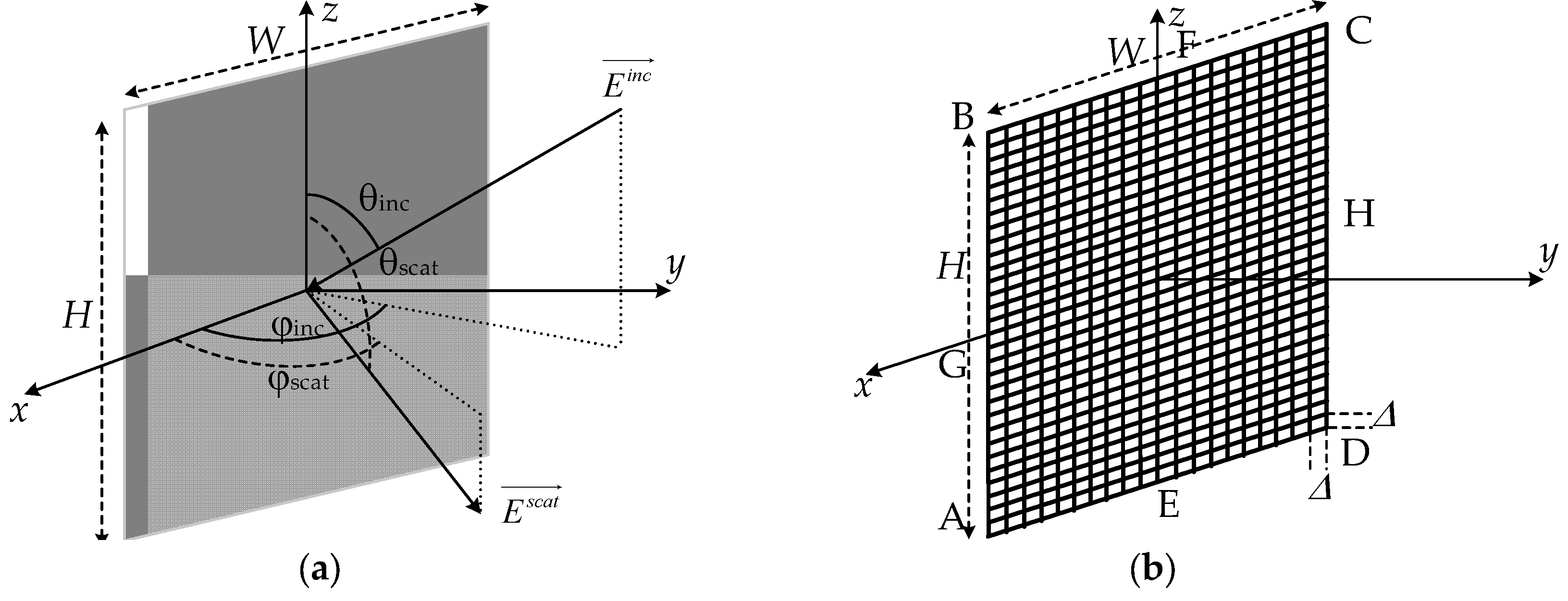
Figure 2.
Measured (●●●) and calculated BSCS results for the scatterer in the xOy (a) and yOz (b) plane using MoM with PBF (?) and PWS (---).
Figure 2.
Measured (●●●) and calculated BSCS results for the scatterer in the xOy (a) and yOz (b) plane using MoM with PBF (?) and PWS (---).
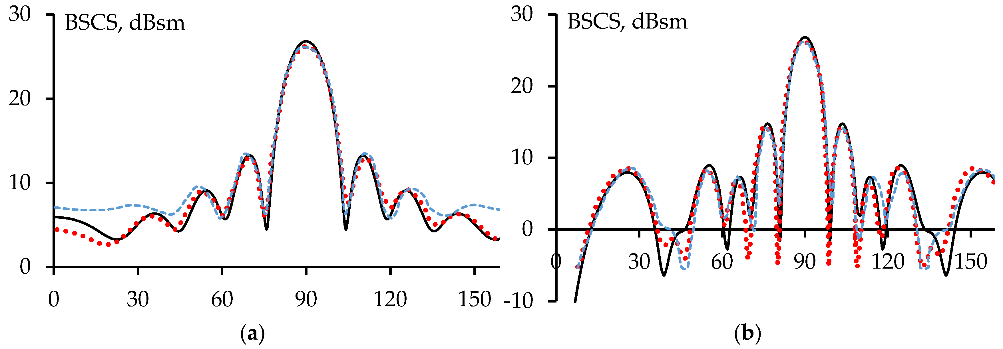
Figure 3.
The dependences of |I| on coordinates along the AB and EF of considered structure when θinc=ϕinc=90°.
Figure 3.
The dependences of |I| on coordinates along the AB and EF of considered structure when θinc=ϕinc=90°.
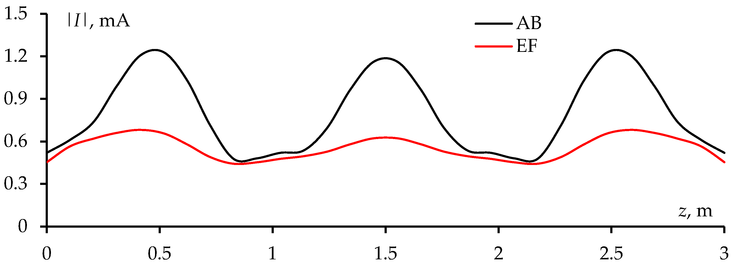
Figure 4.
The OCGA algorithm for creating sparse scatterers when the incident wave is excited in a fixed direction.
Figure 4.
The OCGA algorithm for creating sparse scatterers when the incident wave is excited in a fixed direction.
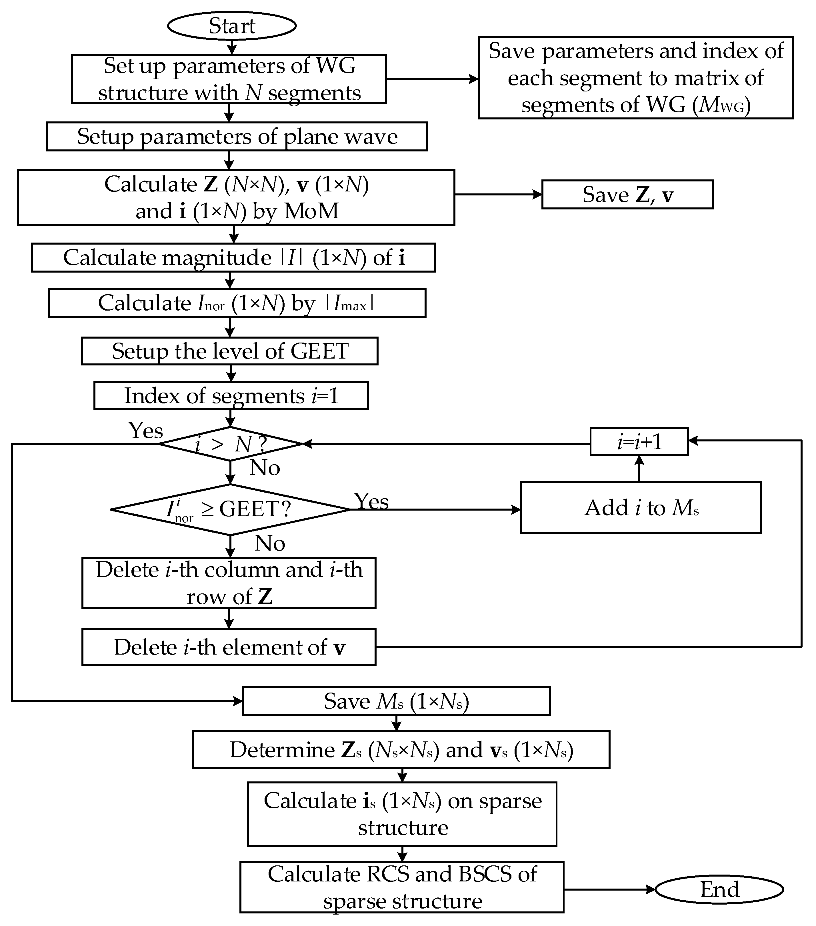
Figure 5.
The dependence of RCSmax on GEET when θinc=ϕinc=90°.
Figure 6.
The GEET dependences of the sparse WG reduction in scatterer mass and surface, and in the time and memory on subsequent simulations after OCGA.
Figure 6.
The GEET dependences of the sparse WG reduction in scatterer mass and surface, and in the time and memory on subsequent simulations after OCGA.
Figure 7.
The MATLAB models of S35 (a), S40 (b), S50 (c).
Figure 8.
The obtained RCSs (a, b) and BSCSs (c, d) for original and sparse structures in xOy (a, c) and yOz (b, d) planes.
Figure 8.
The obtained RCSs (a, b) and BSCSs (c, d) for original and sparse structures in xOy (a, c) and yOz (b, d) planes.
Figure 9.
The OCGA algorithm for creating universal sparse scatterers when the incident wave is excited in region direction.
Figure 9.
The OCGA algorithm for creating universal sparse scatterers when the incident wave is excited in region direction.
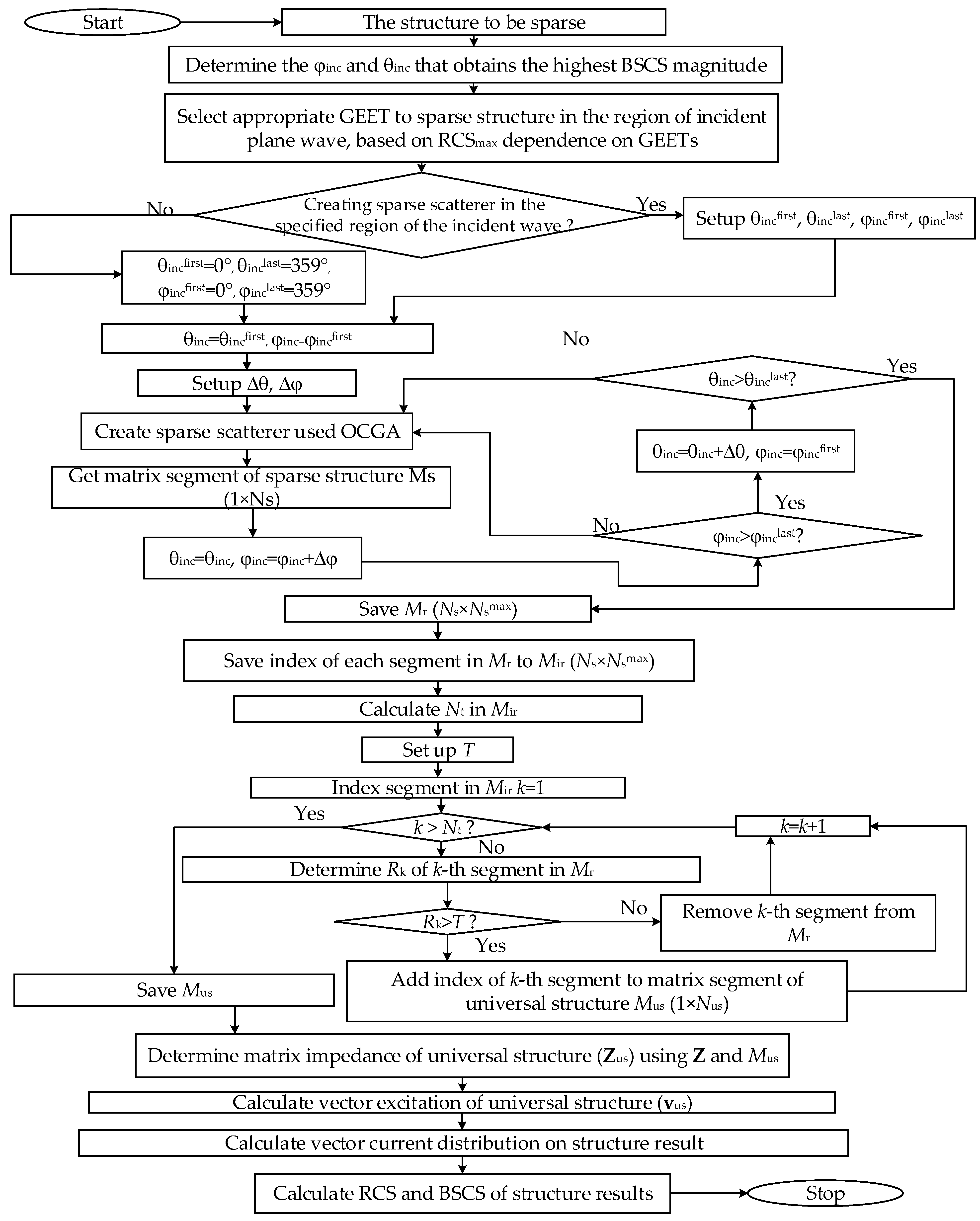
Figure 10.
The MATLAB models of US50 (a), US100 (b), US200 (c), US300 (d).
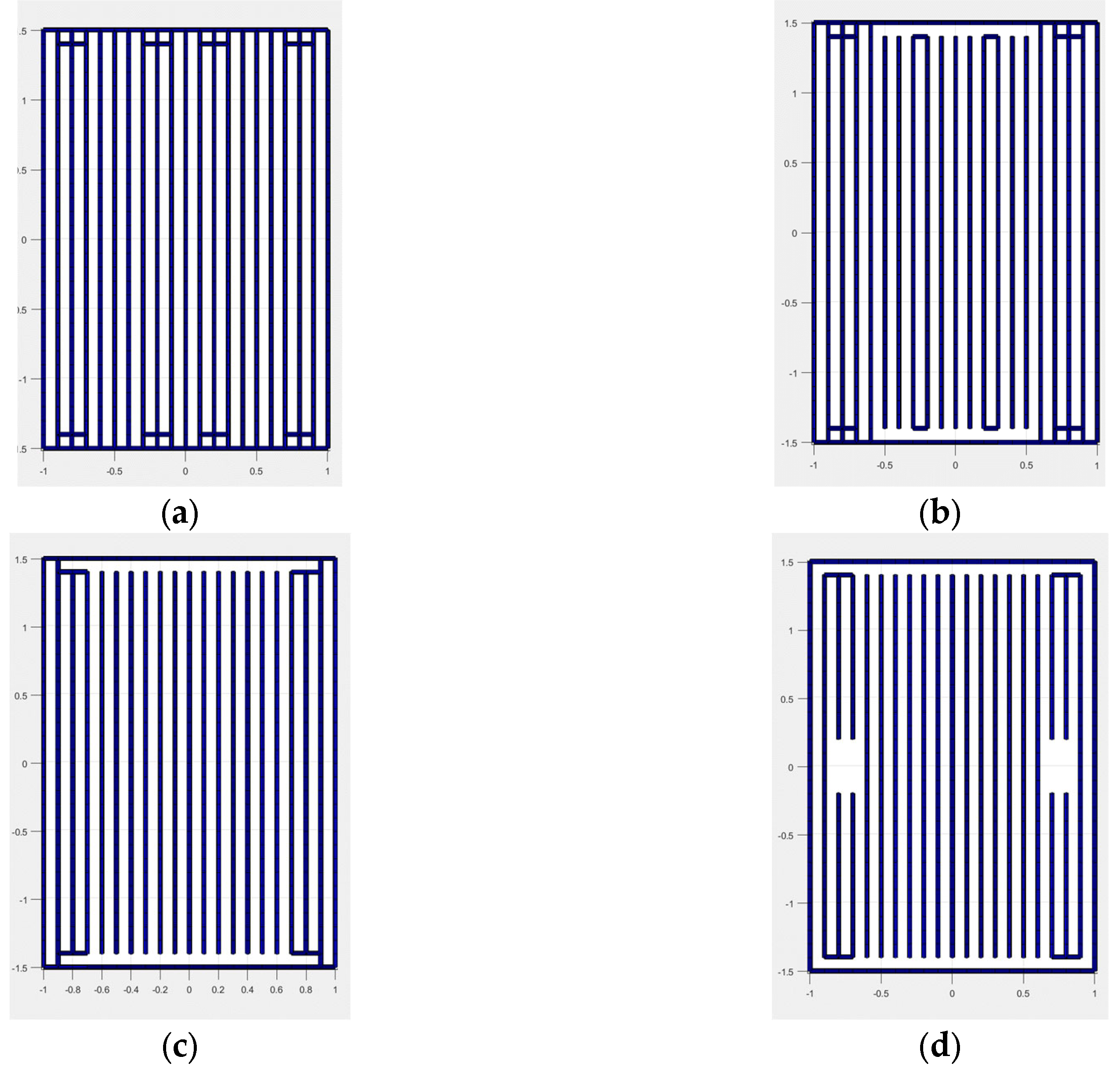
Figure 11.
The obtained BSCSs for original and sparse structures in xOy (a) and yOz (b) planes.
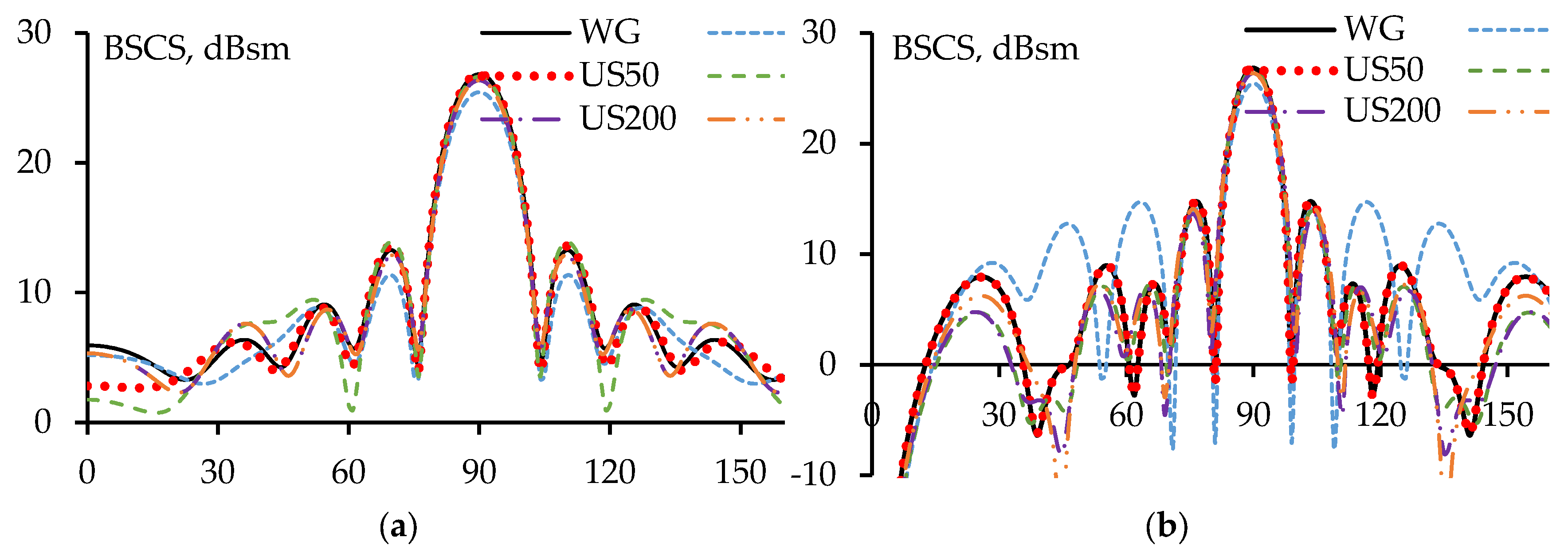
Figure 12.
The dependence of correlation coefficient of group 1 (a) and group 2 (b) on T.
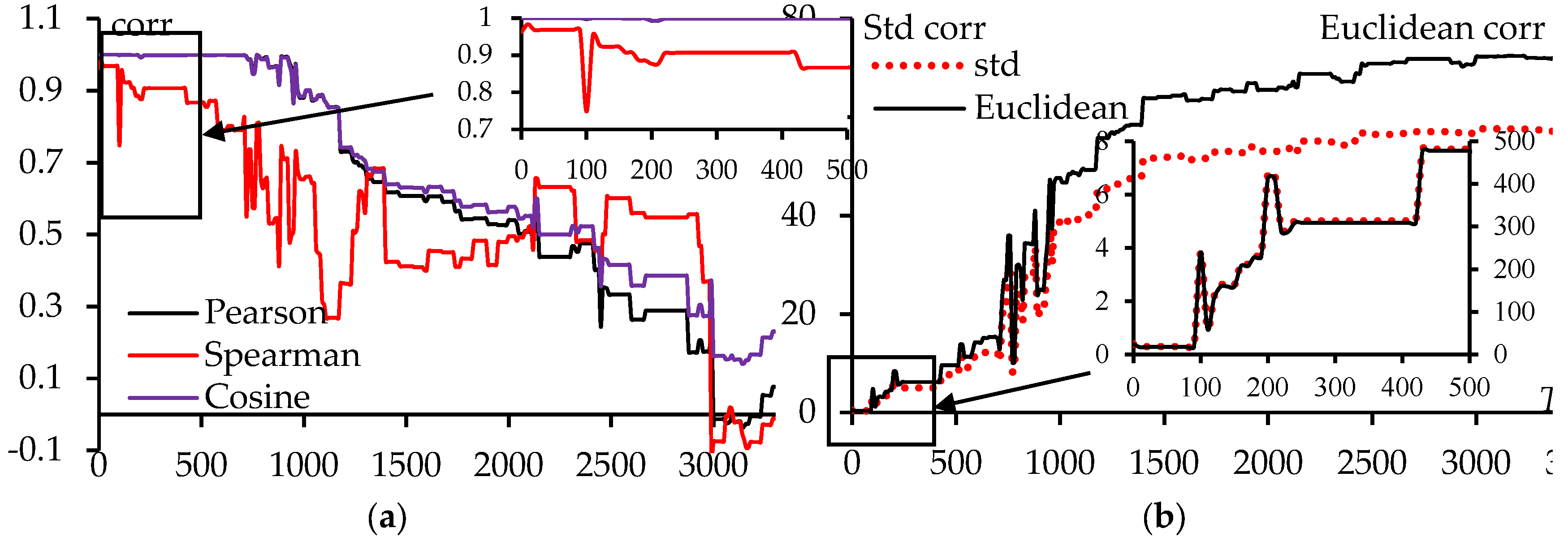
Figure 13.
T dependences of the sparse WG reduction in scatterer mass and surface, and in the time and memory on subsequent simulations after OCGA.
Figure 13.
T dependences of the sparse WG reduction in scatterer mass and surface, and in the time and memory on subsequent simulations after OCGA.
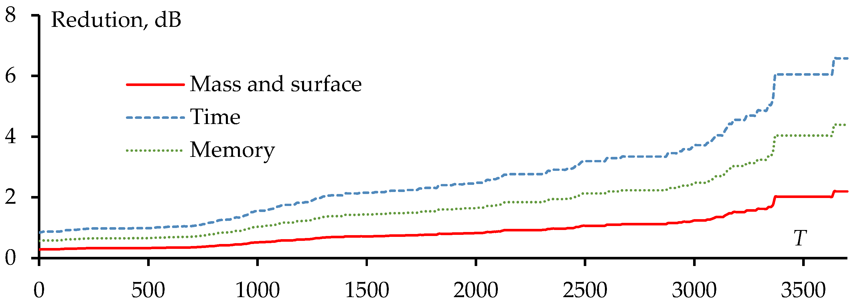
Figure 14.
The MATLAB models of USr50 (a), USr100 (b), USr200 (c), and USr300 (d).
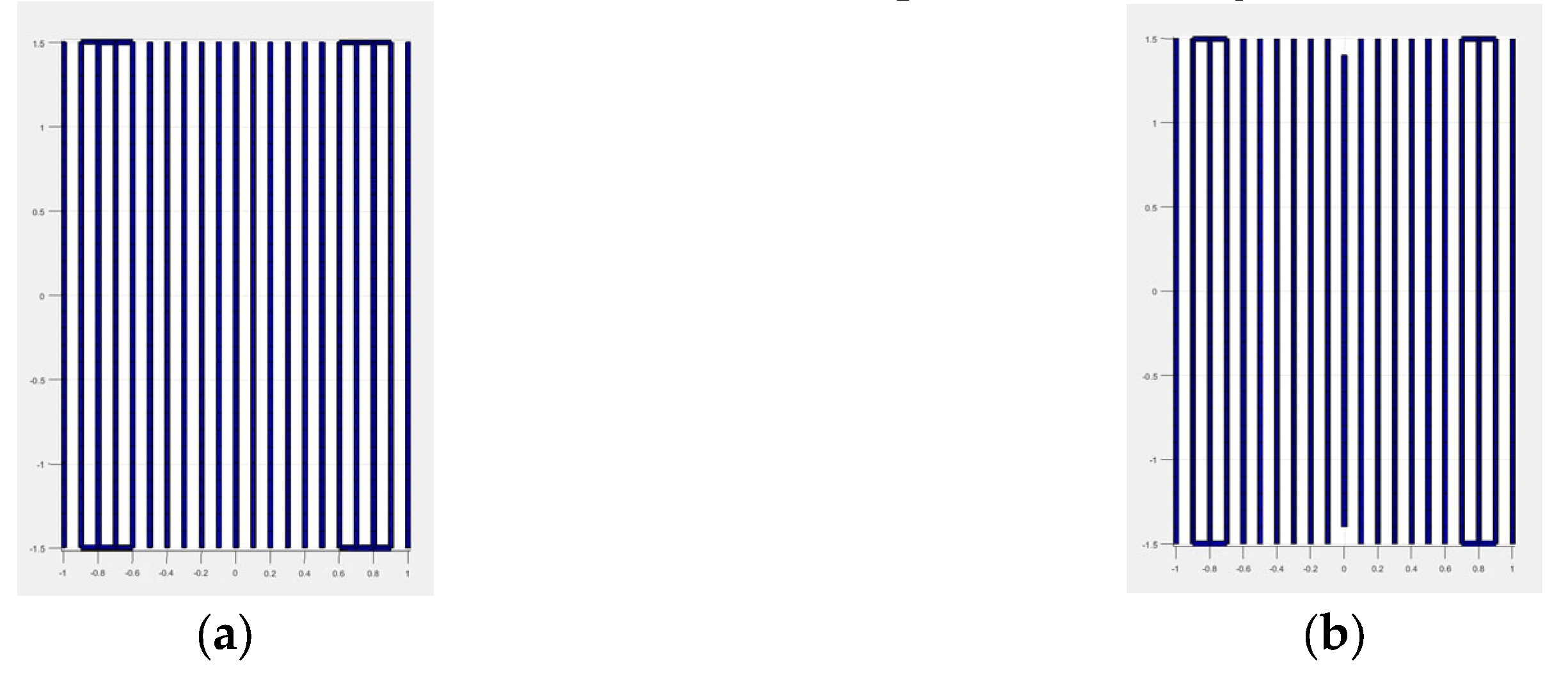
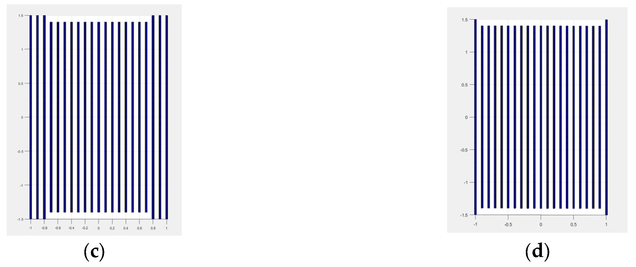
Figure 15.
The obtained BSCSs for original (smoothing value) and sparse structures in region θ=60–120°, ϕ=60–120° (a), xOy (b) and yOz (c) plane.
Figure 15.
The obtained BSCSs for original (smoothing value) and sparse structures in region θ=60–120°, ϕ=60–120° (a), xOy (b) and yOz (c) plane.


Table 1.
Prototype, original WG structure and sparse structures obtained after applying different approaches to different types of antennas.
Table 1.
Prototype, original WG structure and sparse structures obtained after applying different approaches to different types of antennas.
| Antenna | f, GHz | GEET, % | Prototype | Original WG | Sparse after OCGA | Sparse after EOCGA | Sparse after NCOCGA |
|---|---|---|---|---|---|---|---|
| Reflector | 3.4-3.7 [65] | 30 |  |
 |
 |
 |
 |
| 5.1-5.9 [63] | 10 | 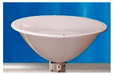 |
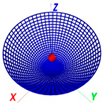 |
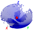 |
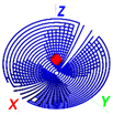 |
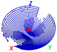 |
|
| 10-12 [64] | 20 | 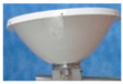 |
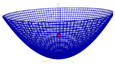 |
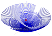 |
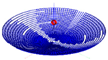 |
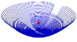 |
|
| Horn | 0.7-1.3 [67] |
75 |  |
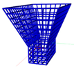 |
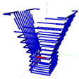 |
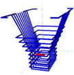 |
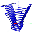 |
| 18-38 [66] |
80 | 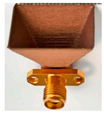 |
 |
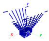 |
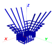 |
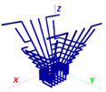 |
|
| Conical horn | 5.3-6.3 [68] |
20 |  |
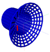 |
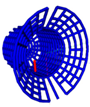 |
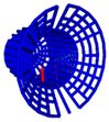 |
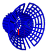 |
| 8 [63] | 6 | 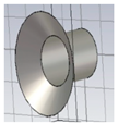 |
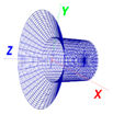 |
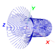 |
 |
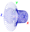 |
|
| Patch | 2-3 [69] | 30 | 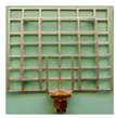 |
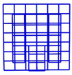 |
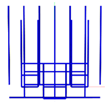 |
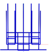 |
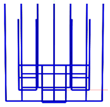 |
Table 2.
The improvements and maximum differences from the original sparse structure after applying different approaches to different antenna types.
Table 2.
The improvements and maximum differences from the original sparse structure after applying different approaches to different antenna types.
| Antenna | f, GHz | GEET, % | Approach | Reductions, times | Maximum difference of characteristics | |||||
| Mass and surface | Memory | Time | Gmax , dB | VSWR | |S11|, dB | |Z|, Ohm | ||||
| Reflector | 3.4–3.7 [65] | 30 | OCGA | 1.39 | 1.94 | 2.71 | 0.14 | 0.007 | 2.83 | 0.34 |
| EOCGA | 1.99 | 3.97 | 7.91 | 3.91 | 0.018 | 8.78 | 0.72 | |||
| NCOCGA | 1.37 | 1.88 | 2.58 | 0.09 | 0.006 | 3.30 | 0.29 | |||
| 5.1–5.9 [63] | 10 | OCGA | 1.51 | 2.28 | 3.44 | 0.12 | 0.01 | 0.26 | 0.08 | |
| EOCGA | 1.80 | 3.24 | 5.84 | 2.20 | 0.01 | 0.13 | 0.46 | |||
| NCOCGA | 1.49 | 2.21 | 3.27 | 0.10 | 0.01 | 0.25 | 0.09 | |||
| 10–12 [64] | 20 | OCGA | 1.37 | 1.87 | 2.57 | 0.30 | 0.014 | 0.63 | 0.54 | |
| EOCGA | 1.78 | 3.17 | 5.64 | 3.47 | 0.032 | 0.85 | 1.48 | |||
| NCOCGA | 1.36 | 1.86 | 2.53 | 0.28 | 0.016 | 0.61 | 0.70 | |||
| Horn | 0.7–1.3 [67] |
75 | OCGA | 1.86 | 3.45 | 6.40 | 2.38 | 1.20 | 14.64 | 30.45 |
| EOCGA | 2.03 | 4.11 | 8.32 | 3.14 | 1.11 | 12.51 | 31.02 | |||
| NCOCGA | 1.83 | 3.35 | 6.14 | 2.33 | 1.22 | 13.00 | 28.14 | |||
| 8–12 [61] | 60 | OCGA | 1.58 | 2.50 | 3.94 | 2.75 | 3.62 | 0.19 | 7.28 | |
| COCGA | 1.56 | 2.44 | 3.82 | 2.04 | 3.17 | 0.16 | 7.33 | |||
| 18–38 [66] |
80 | OCGA | 2.36 | 5.56 | 13.11 | 2.22 | 0.51 | 3.24 | 6.51 | |
| EOCGA | 2.46 | 6.05 | 14.89 | 2.41 | 0.48 | 3.22 | 6.74 | |||
| NCOCGA | 2.32 | 5.38 | 12.48 | 2.20 | 0.46 | 3.14 | 6.15 | |||
| Conical horn | 5.3–6.3 [68] |
20 | OCGA | 1.19 | 1.42 | 1.69 | 1.67 | 0.53 | 2.32 | 22.98 |
| EOCGA | 1.19 | 1.42 | 1.69 | 1.67 | 0.53 | 2.32 | 22.98 | |||
| NCOCGA | 1.19 | 1.42 | 1.69 | 1.67 | 0.53 | 2.32 | 22.98 | |||
| 8 [63] | 6 | OCGA | 1.26 | 1.60 | 2.02 | 0.55 | 0.03 | 0.21 | 0.24 | |
| EOCGA | 2.75 | 7.55 | 20.75 | 3.91 | 0.22 | 1.44 | 29.28 | |||
| NCOCGA | 1.25 | 1.56 | 1.96 | 0.57 | 0.03 | 0.22 | 0.20 | |||
| Patch | 2–3 [69] | 30 | OCGA | 1.52 | 2.31 | 3.51 | 0.22 | 2.79 | 6.04 | 41.49 |
| EOCGA | 1.72 | 2.95 | 5.07 | 1.54 | 11.52 | 15.88 | 66.63 | |||
| NCOCGA | 1.49 | 2.22 | 3.31 | 0.88 | 3.08 | 15.81 | 136.12 | |||
Table 3.
The improvements and maximum differences from the original sparse structure after applying different approaches to different antenna types.
Table 3.
The improvements and maximum differences from the original sparse structure after applying different approaches to different antenna types.
| Antenna | f, GHz | Approach for reduction | Approach for characteristics | Current distribution for sparse structure | Frequency for characteristics |
| Reflector | 3.4–3.7 [65] | E/OCGA | NCOCGA | at the lowest frequency | at the center frequencies |
| 10–12 [64] | E/OCGA | NCOCGA | at the lowest frequencies | at higher frequencies | |
| Horn | 0.7–1.3 [67] | E/OCGA | NCOCGA | at the center and lowest frequency | at higher frequencies |
| 8–12 [61] | OCGA | COCGA | at the lowest frequencies | at higher frequencies | |
| 18–38 [66] | E/OCGA | NCOCGA | at the lowest or center frequencies | at higher frequencies | |
| Conical horn | 5.3–6.3 [68] | E/OCGA | NCOCGA | at the lowest or center frequencies | at lowest and higher frequencies |
| Patch | 2–3 [69] | E/OCGA | NCOCGA | at low and center frequencies | at a particular frequency |
Table 4.
RCSs, BSCSs, and bandwidth deviations for S35, S40, and S50.
| Structure | Deviation | Maximum deviation, dBsm | ||||||
|---|---|---|---|---|---|---|---|---|
| xOy | yOz | xOy | yOz | |||||
| RCSmax, dBsm | BW, ° | RCSmax, dBsm | BW, ° | RCS | BSCS | RCS | BSCS | |
| S35 | 0.032 | 0 | 0.032 | 0 | 0.5 | 1.7 | 0.52 | 3.14 |
| S40 | 1.388 | 0 | 1.388 | 0 | 1.54 | 2.45 | 6.82 | 17.14 |
| S50 | 10.89 | 30 | 10.89 | 2 | 10.89 | 10.89 | 19.77 | 22.89 |
Table 5.
BSCS (dBsm) deviations for S40, US50, US100, US200, and US300.
| Structure | BSCSmax | Maximum BSCS deviation | |
|---|---|---|---|
| xOy and yOz | xOy | yOz | |
| S40 | 1.39 | 2.45 | 17.1 |
| US50 | 0.000187 | 3.11 | 0.25 |
| US100 | 0.194 | 4.77 | 6.46 |
| US200 | 0.479 | 1.554 | 8.89 |
| US300 | 0.479 | 1.554 | 13.7 |
Table 6.
BSCS (dBsm) deviations for S40, S50, S100, S200, and S300.
| Structure | BSCSmax | Maximum BSCS deviation | ||
|---|---|---|---|---|
| θ=60–120°, ϕ=60–120° | xOy plane | yOz plane | ||
| S40 | 1.388 | 31.17 | 2.45 | 17.14 |
| S50 | 0.0003 | 18.15 | 1.98 | 0.37 |
| S100 | 0.014 | 28.51 | 2.1 | 19.58 |
| S200 | 0.33 | 23.45 | 2.2 | 12.84 |
| S300 | 0.42 | 18.55 | 1.8 | 8.15 |
Disclaimer/Publisher’s Note: The statements, opinions and data contained in all publications are solely those of the individual author(s) and contributor(s) and not of MDPI and/or the editor(s). MDPI and/or the editor(s) disclaim responsibility for any injury to people or property resulting from any ideas, methods, instructions or products referred to in the content. |
© 2024 by the authors. Licensee MDPI, Basel, Switzerland. This article is an open access article distributed under the terms and conditions of the Creative Commons Attribution (CC BY) license (http://creativecommons.org/licenses/by/4.0/).
Copyright: This open access article is published under a Creative Commons CC BY 4.0 license, which permit the free download, distribution, and reuse, provided that the author and preprint are cited in any reuse.


