Submitted:
17 December 2024
Posted:
18 December 2024
You are already at the latest version
Abstract
In the current work, we analyze the spectral distribution of the geometric mean of two or more matrix-sequences constituted by Hermitian positive definite matrices, under the assumption that all input matrix-sequences belong to the same Generalized Locally Toeplitz (GLT) $*$-algebra. We consider the geometric mean for two matrices, using the Ando-Li-Mathias (ALM) definition, and then we pass to the extension of the the idea to more than two matrices by introducing the Karcher mean. While there is no simple formula for the geometric mean of more than two matrices, iterative methods from the literature are employed to compute it. The main novelty of the work is the extension of the study in the distributional sense when input matrix-sequences belong to one of the GLT $*$-algebras. More precisely, we show that the geometric mean of more than two positive definite GLT matrix-sequences forms a new GLT matrix-sequence, with the GLT symbol given by the geometric mean of the individual symbols. Numerical experiments are reported concerning scalar and block GLT matrix-sequences in both one-dimensional and two-dimensional cases. A section with conclusions and open problems ends the current work.
Keywords:
Matrix geometric mean
; Karcher mean
; Positive definite matrix
; multilevel Toeplitz matrices
; generalized locally Toeplitz sequences
1. Introduction
The study of geometric means of matrices has become increasingly important in various fields, including numerical linear algebra, differential equations, and signal processing. Positive definite matrices arise naturally in many applications, such as in the discretization of differential equations via methods like finite differences or finite elements. These methods produce matrix-sequences whose sizes increase as the mesh size becomes finer. An essential concept related to matrix-sequences is the asymptotic eigenvalue distribution in the Weyl sense and this has been a classical study; see e.g. [17,23,40]. Since the publication of the seminal papers by Tyrtyshnikov in 1996 [41] and Tilli in 1998 [38,39], there has been growing interest in this area, which eventually contributed to the development of the theory of Generalized Locally Toeplitz (GLT) sequences [35,36]. The increasing attention to this topic is not purely theoretical, as the asymptotic eigenvalue and singular value distributions have significant practical applications, particularly in the analysis of large-scale matrix computations especially in the context of the numerical approximations of systems of (fractional) partial differential equations ((F)PDEs); see e.g. the books and review papers [7,8,20,21,22] and references therein. In fact, it is worth noticing that virtually any meaningful approximation technique of a (F)PDE leads to a GLT matrix-sequence, including finite differences, finite elements of any order, discontinuous Galerkin techniques, finite volumes, isogeometric analysis etc. More in detail, if we fix positive integer numbers, then the set of d-level r-block GLT matrix-sequences forms a maximal *-algebra of matrix-sequences, isometrically equivalent to d-variate matrix-valued mesurable functions defined on . Furthermore, a d-level r-block GLT sequence is uniquely associated with a matrix-valued Lebesgue-measurable function , known as the GLT symbol, which is defined over the domain . Notice that the set can be replaced by any bounded Peano-Jordan measurable subset of as occurring with the notion of reduced GLT *-algebras, see [35][pp. 398-399, formula (59)] for the first occurrence with applications of approximated PDEs on general non-Cartesian domains in d dimensions, [36][Section 3.1.4] for the first formal proposal, and [5] for an exhaustive treatment, containing both the *-algebra theoretical results and a number of applications. This symbol provides a powerful tool for analyzing the singular value and eigenvalue distributions when the matrices are Hermitian and part of a matrix-sequence of increasing size. The notation indicates that is a GLT sequence with symbol . Notably, the symbol of a GLT sequence is unique in the sense that if and , then almost everywhere in [7,8,20,21]. Furthermore, by the *-algebra structure, and implies that , i.e., the matrix-sequence is zero-distributed and the latter is very important for building explicit matrix-sequences approximating a GLT matrix-sequence and whose inversion is computationally cheap, in the context of preconditioning of large linear systems.
In certain physical applications, it is often necessary to represent the results of multiple experiments through a single average matrix G, where the data is represented by a set of positive definite matrices . The arithmetic mean is not appropriate in these cases because it does not fulfill the requirement that the inverse of the mean should coincide with the average of the inverses . This property, which is crucial in certain physical models is satisfied by the geometric mean. For positive real numbers , the geometric mean is defined as
a concept that is extended to the case of matrices [10,26] in a nontrivial way, where the difficulty is of course the lack of commutativity. A well-known definition that satisfies desirable properties such as congruence invariance, permutation invariance, and consistency with the scalar geometric mean was proposed by ALM [1]. They defined the geometric mean of two Hermitian positive definite (HPD) matrices as
We recall the definition of functions applied to diagonalizable matrices, which we frequently utilize throughout our work. Suppose is diagonalizable, meaning , where is a diagonal matrix, and f is a given function. In this case, is defined as , with being a diagonal matrix whose diagonal entries are , for . In the case where f is a multi-valued function, the same branch of f must be chosen for any repeated eigenvalue.
If then the ALM-mean is obtained through a recursive iteration process where at each step the geometric means of k matrices are computed by reducing them to matrices. However, a significant limitation of this method is its linear convergence leading to a high computational cost due to the large number of iterations required at each recursive step. As a result, the computation of the ALM-mean using this approach becomes quite expensive. However, despite the elegance of the ALM geometric mean for two matrices, it becomes computationally infeasible to extend this formula to more than two matrices [14].
To overcome these limitations, the Karcher mean [13], was introduced as a generalization of the geometric mean for more than two matrices. The Karcher mean of HPD matrices is defined as the unique positive definite solution to the matrix equation:
as established by Moakher [26, Proposition 3.4]. This equation can be equivalently expressed in other forms, such as
by utilizing the formula , which holds for any invertible matrix M and any matrix K with real positive eigenvalues. This formulation arises from Riemannian geometry, where the space of positive definite matrices forms a Riemannian manifold with non-positive curvature. The Karcher mean represents the center of mass (or barycenter) on this manifold [10]. In this manifold, the distance between two positive definite matrices A and B is defined as where denotes the Frobenius norm.
Several numerical methods have been proposed for solving the Karcher mean equation. Initially, fixed-point iteration methods were used, but these methods suffered from slow convergence, especially in cases where the matrices involved were poorly conditioned [26]. Later, methods based on gradient descent in the Riemannian manifold were introduced. A common iteration scheme for approximating the Karcher mean is
where is the approximation at the v-th step, and the exponential and logarithmic functions are matrix operations. Although this method improves convergence, it can exhibit slow linear convergence in certain cases. The iteration with or and , as considered in [25,26], can fail to converge for some matrices . Furthermore, similar iterations have been proposed in [3,28], but without specific recommendations on choosing the initial value or step length. While an optimal could theoretically be determined using a line search strategy, this approach is often computationally expensive. Heuristic strategies for selecting the step size, as discussed in [18], may result in slow convergence in many cases.
To further enhance the convergence rate, the Richardson iteration method is employed. Indeed, the considered method improves the convergence by using a parameter , which controls the step size in each iteration [13]. More precisely, given , the Richardson iteration is given by
Any solution of Eq. (3) is a fixed point of the map T in (5). The iterative formula can also be rewritten as
provided that all the iterates remain positive definite. Equation (6) further demonstrates that if is Hermitian, then is also a Hermitian matrix.
The parameter plays a crucial role in controlling the step size of each iteration and choosing an optimal value of can significantly influence the convergence behavior of the iteration. If is small enough, the iteration is guaranteed to produce positive definite matrices and converge towards the solution. In particular, when the matrices commute, setting ensures at least quadratic convergence. More generally, the optimal value of can be determined based on the condition numbers of matrices , where G is the desired solution. The closer the eigenvalues of are to 1, the faster the convergence is. This analysis guarantees that if the initial guess is close enough to the solution and is positive definite, the sequence generated by the iteration remains well-defined and converges to the desired solution. However, if the initial iterate is not positive definite, adjusting the value of or modifying the iteration scheme may be necessary to ensure that all iterates remain positive.
Numerical experiments show that selecting appropriate initial guesses, such as the arithmetic mean or the identity matrix , can significantly affect the convergence rate. In particular, the cheap mean introduced in [12] provides a practical initial approximation that leads to faster convergence in many cases.
In our study, we consider the analysis of the Karcher mean to matrix-sequences, particularly those arising from the discretization of differential equations, which often form GLT sequences. Numerical results demonstrate that the geometric mean of not only two but more than two GLT matrix-sequences is itself a GLT matrix-sequence, with the symbol of the new sequence given by the geometric mean of the original symbols: the latter is formally proven in the case of two GLT matrix-sequences. Regarding the examples, we consider either scalar unilevel and multilevel GLT matrix-sequences or block GLT asymptotic structures, with special attention to cases stemming from the approximation by local methods of differential operators. By analyzing the spectral distribution of the geometric mean of these matrix-sequences, we provide new insights into the asymptotic behavior of large-scale matrix computations and their potential applications in numerical analysis.
This paper is structured as follows. In Section 2, we introduce notations, terminology, and preliminary results concerning Toeplitz and GLT structures, which are essential for the mathematical formulation of the problem and its technical solution. In Section 3, we present the geometric mean of two matrices and the Karcher mean for more than two matrices, followed by a discussion of the iterative methods employed for their computation: the section contains the GLT theoretical results. Section 4 contains numerical experiments that illustrate the (asymptotic) spectral behavior of the geometric mean for GLT matrix-sequences in both 1D and 2D settings and in both scalar and block cases. Finally, in Section 5 we draw conclusions and we punt in evidence few open problems.
2. Preliminaries
In this introduction, we provide the necessary tools for performing the spectral analysis of the matrices involved, based on the theory of uni and multilevel block GLT matrix-sequences.
2.1. Matrices and Matrix-Sequences
Given a square matrix , we denote by its conjugate transpose and by the Moore–Penrose pseudoinverse of A. Recall that whenever A is invertible. Regarding matrix norms refers to the spectral norm and for , the notation stands for the Schatten p-norm defined as the p-norm of the vector of the singular values. Note that the Schatten ∞-norm, which is equal to the largest singular value coincides with the spectral norm ; the Schatten 1-norm since it is the sum of the singular values is often referred to as the trace-norm; and the Schatten 2-norm coincides with the Frobenius norm. Schatten p-norms, as important special cases of unitarily invariant norms are treated in detail in a wonderful book by Bhatia [9].
Finally, the expression matrix-sequence refers to any sequence of the form , where is a square matrix of size with strictly increasing so that as . A r-block matrix-sequence, or simply a matrix-sequence if r can be deduced from context is a special in which the size of is , with fixed and strictly increasing.
2.2. Multi-Index Notation
To effectively deal with multilevel structures it is necessary to use multi-indices, which are vectors of the form . The related notation is listed below
- are vectors of all zeroes, ones, twos, etc.
- means that for all . In general, relations between multi-indices are evaluated componentwise.
- Operations between multi-indices, such as addition, subtraction, multiplication, and division, are also performed componentwise.
- The multi-index interval is the set . We always assume that the elements in an interval are ordered in the standard lexicographic manner
- means that varies from to , always following the lexicographic ordering.
- means that .
- The product of all the components of is denoted as .
A multilevel matrix-sequence is a matrix-sequence such that n varies in some infinite subset of , is a multi-index in depending on n, and when . This is typical of many approximations of differential operators in d dimensions.
2.3. Singular Value and Eigenvalue Distributions of a Matrix-Sequence
Let be the Lebesgue measure in . Throughout this work, all terminology from measure theory (such as “measurable set,” “measurable function,” “almost everywhere”, etc.) always refers to the Lebesgue measure. Let (resp., ) be the space of continuous complex-valued functions with bounded support defined on (resp., ). If , the singular values and eigenvalues of A are denoted by and , respectively. The set of the eigenvalues (i.e., the spectrum) of A is denoted by .
Definition 1.
(Singular value and eigenvalue distribution of a matrix-sequence). Let be a matrix-sequence, with of size , and let be a measurable function defined on a set D with .
- We say that has an (asymptotic) singular value distribution described by ψ, and we write , if
- We say that has an (asymptotic) spectral (or eigenvalue) distribution described by ψ, and we write , if
- If ψ describes both the singular value and eigenvalue distribution of , we write .
In this case, the function ψ is referred to as the eigenvalue (or spectral) symbol of .
The same definition when the considered matrix-sequence shows a multilevel structure. In that case n is replaced by uniformly in and .
The informal meaning behind the spectral distribution definition is as follows: if is continuous, then a suitable ordering of the eigenvalues , assigned in correspondence with an equispaced grid on D, reconstructs approximately the r surfaces , . For example, in the simplest case where and , , the eigenvalues of are approximately equal — up to a few potential outliers — to , where
If and , , the eigenvalues of are approximately equal — again up to a few potential outliers — to , where
If the considered structure is two-level then the subscript is and .
Furthermore, for , a similar reasoning applies.
Finally we report an observation which is useful in the following derivations.
Remark 1.
The relation and for all n imply that the range of f is a subset of the closure of S. In particular and positive definite for all n imply that f is nonnegative definite almost everywhere, simply nonnegative almost everywhere if . The same applies when a multilevel matrix-sequence is considered and similar statements hold when singular values are taken into account.
2.4. Approximating Classes of Sequences
In this subsection, we present the notion of the approximating class of sequences and a related key result.
Definition 2
(Approximating class of sequences). Let be a matrix-sequence and let be a class of matrix-sequences, with and of size . We say that is an approximating class of sequences (a.c.s.) for if the following condition is met: for every j, there exists such that, for every ,
where , , and depend only on j, and
denotes that is an a.c.s. for .
The following theorem represents the expression of a related convergence theory and it is a powerful tool used, for example, in the construction of the GLT *-Algebra
Theorem 1.
Let , , with , be matrix-sequences and let be measurable functions defined on a set D with positive and finite Lebesgue measure. Suppose that:
- 1.
- for every j;
- 2.
- ;
- 3.
- in measure.
Then
Moreover, if all the involved matrices are Hermitian, the first assumption is replaced by for every j, and the other two are left unchanged, then
We end this section by observing that the same definition can be given and corresponding results (with obvious changes) hold, when the involved matrix-sequences show a multilevel structure. In that case n is replaced by uniformly in , , .
2.5. Matrix-Sequences with Explicit or Hidden (Asymptotic) Structure
In this subsection, we introduce the three types of matrix structures that constitute the basic building blocks of the GLT *-algebras. To be more specific, for any positive integers we consider the set of d-level r-block GLT matrix-sequences. For any positive integers, the considered set forms a *-algebra of matrix-sequences, which is maximal and is isometrically equivalent to the maximal *-algebra of -variate matrix-valued measurable functions (with respect to the Lebesgue measure) defined canonically over ; see [4,7,8,19,20,21] and references therein.
The reduced version is essential when dealing with approximations of integro-differential operators (also in fractional versions) defined over general (non-Cartesian) domains. The idea was presented in [35,36] and it was exhaustively developed in [5], where the GLT symbols are again measurable functions defined over , with Peano-Jordan measurable and contained in . Als the reduced versions form maximal *-algebras isometrically equivalent to the corresponding maximal *-algebras of measurable functions. The considered GLT *-algebras represent rich examples of hidden (asymptotic) structures. Their building blocks are formed by two classes of explicit algebraic structures, d-level r-block Toeplitz and sampling diagonal matrix-sequences (see Section 2.7 and Section 2.8), plus the asymptotic structures given by the zero-distributed matrix-sequences; see Section 2.6. It is worth noticing that the latter class plays the role of compact operators with respect to bounded linear operators and in fact they form a two-sided ideal of matrix-sequences with respect to any of the GLT *-algebras.
2.6. Zero-Distributed Sequences
Zero-distributed sequences are defined as matrix-sequences such that . Note that, for any , is equivalent to , where is the zero matrix. The following theorem (see [34] and [20]), provides a useful characterization for detecting this type of sequence. We use the natural convention .
Theorem 2.
Let be a matrix-sequence, with of size . Then
- if and only if with and as ;
- if there exists such that as .
As in Section 2.4, the same definition can be given and corresponding result (with obvious changes) holds, when the involved matrix-sequences show a multilevel structure. In that case n is replaced by uniformly in .
2.7. Multilevel Block Toeplitz Matrices
Given , a matrix of the form
with blocks , , is called multilevel block Toeplitz, or more precisely, d-level r-block Toeplitz matrix.
Given a matrix-valued function belonging to , the -th Toeplitz matrix associated with f is defined as
where
are the Fourier coefficients of f, in which i denotes the imaginary unit, the integrals are computed componentwise, and . Equivalently, can be expressed as
where ⊗ denotes the Kronecker tensor product between matrices and is the matrix of order m whose entry equals 1 if and zero otherwise.
is the family of (multilevel block) Toeplitz matrices associated with f, which is called the generating function.
2.8. Block Diagonal Sampling Matrices
Given , , and a function , we define the multilevel block diagonal sampling matrix as the block diagonal matrix
2.9. The *-Algebra of d-Level r-Block GLT Matrix-Sequences
Let be a fixed integer. A multilevel r-block GLT sequence, or simply a GLT sequence if we do not need to specify r, is a special multilevel r-block matrix-sequence equipped with a measurable function , , called symbol. The symbol is essentially unique, in the sense that if are two symbols of the same GLT sequence, then almost everywhere. We write to denote that is a GLT sequence with symbol .
It can be proven that the set of multilevel block GLT sequences is the *-algebra generated by the three classes of sequences defined in Section 2.6, Section 2.7, Section 2.8: zero-distributed, multilevel block Toeplitz, and block diagonal sampling matrix-sequences. The GLT class satisfies several algebraic and topological properties that are treated in detail in [7,8,20,21]. Here, we focus on the main operative properties, listed below, that represent a complete characterization of GLT sequences, equivalent to the full constructive definition.
GLT Axioms
- GLT 1. If then in the sense of Definition 1, with and . Moreover, if each is Hermitian, then , again in the sense of Definition 1 with .
-
GLT 2. We have
- -
- if is in ;
- -
- if is Riemann-integrable;
- -
- if and only if .
-
GLT 3. If and , then:
- -
- ;
- -
- for all ;
- -
- ;
- -
- , provided that is invertible almost everywhere.
- GLT 4. if and only if there exist such that and in measure.
-
GLT 5. If and , where
- -
- every is Hermitian,
- -
- for some constant C independent of n,
- -
- ,
then . - GLT 6. If and each is Hermitian, then for every continuous function .
Note that, by GLT 1, it is always possible to obtain the singular value distribution from the GLT symbol, while the eigenvalue distribution can only be deduced either if the involved matrices are Hermitian or the related matrix-sequence is quasi-Hermitian in the sense of GLT 5.
3. Geometric Mean of GLT Matrix-Sequences
This section discusses the geometric mean of positive definite matrices, starting with the well-established case of two matrices and then considering multiple matrices. In particular we give distribution results in the case of GLT matrix-sequences.
3.1. Means of Two Matrices
The geometric mean of two positive numbers a and b is simply , a fact well-known from basic arithmetic. However, extending this concept to HPD matrices introduces a number of challenges, as matrix multiplication is not commutative. The question of how to define a geometric mean for matrices in a way that preserves key properties such as congruence invariance, consistency with scalars, and symmetry was solved by ALM [1]. Their work presented an axiomatic approach to defining the geometric mean of two HPD matrices previously defined in Equation (1). ALM formalized the geometric mean for matrices by establishing a set of ten essential properties, known as the ALM axioms. These axioms ensure the geometric mean behaves appropriately in the matrix setting. Here are three key properties:
1. Permutation invariance: for all .
2. Congruence invariance: for all and all invertible matrices .
3. Consistency with scalars: for all commuting (note that for all commuting because and is similar to the HPD matrix ).
When considering sequences of matrices, particularly in the framework of GLT sequences, the geometric mean operation is well-preserved under the structure of GLT sequences. If and we consider two scalar unilevel GLT matrix-sequences, that is, and , where are HPD matrices for every n, the matrix-sequence of their geometric mean also forms a scalar unilevel GLT matrix-sequence. The symbol of the resulting sequence is the geometric mean of the individual symbols and .
Theorem 3
([20], Theorem 10.2). Let . Suppose and , where for every n. Assume that at least one between κ and ξ is nonzero almost everywhere. Then
and
The previous result is easily extended to the case of matrix-sequence resulting from the geometric mean of two block multilevel GLT matrix-sequences, thanks to powerful *-algebra structures of considered spaces described in Section 2.9. Indeed the following two generalizations of Theorem 3 hold.
Theorem 4.
Let and . Suppose and , where for every multi-index . Assume that at least one between κ and ξ is nonzero almost everywhere. Then
and
Proof. Since both and are positive definite for every multi-index , the matrix-sequence is well defined according to formula (1) since is well defined for every multi-index . According to the assumption, we start with the case where is nonzero almost everywhere. Hence the matrix-sequence is a GLT matrix-sequence with GLT symbol by Axiom GLT 3, part 3. Since the square root is continuous and well defined over positive definite matrices also the matrix-sequence is a GLT matrix-sequence with GLT symbol by virtue of Axiom GLT 6.
Now using two times GLT 3, part 2, we infer that is a GLT matrix-sequence with GLT symbol , where is positive definite because of the Sylvester inertia law. Hence the square root of is well defined and by exploiting again Axiom GLT 6 we deduce that is a GLT matrix-sequence with GLT symbol . Finally, by exploiting Axiom GLT 3, part 3, we have is a GLT matrix-sequence with GLT symbol and the application of GLT 3, part 2, two time leads to the desired conclusion
where the latter and Axiom GLT 3 imply .
Finally the other case where is nonzero almost everywhere has the very same proof since is invariant under permutations and hence
so that the the same steps can be repeated by exchanging and . •
Theorem 5.
Let . Suppose and , where for every multi-index . Assume that at least one between the minimal eigenvalue of κ and the minimal eigenvalue of ξ is nonzero almost everywhere. Then
and
Furthermore whenever the GLT symbols κ and ξ commute.
Proof. The case of is already contained in Theorem 4, so we assume i.e. a true GLT block setting. The proof is in fact a repetition of that of the previous theorem with the only attention to GLT symbol part where the multiplication is noncommutative.
Since both and are positive definite for every multi-index , the matrix-sequence is well defined according to formula (1) since is well defined for every multi-index . According to the assumption, we start with the case where is invertible almost everywhere so that by Axiom GLT 3, part 3, and thanks to Axiom GLT 6.
Now using two times GLT 3, part 2, we have , where
is positive definite because of the Sylvester inertia law. Hence the square root of is well defined and by exploiting again Axiom GLT 6 we obtain . Finally, by exploiting Axiom GLT 3, part 3, on the matrix-sequence and using GLT 3, part 2, two times, we conclude
where the symbol is exactly . Furthermore, relation (11) and Axiom GLT 3 imply where , whenever and commute.
Finally the remaining case where is invertible almost everywhere has the very same proof since is invariant under permutations and hence
so that the the same steps can be repeated by exchanging and and by exchanging and . •
3.2. Mean of More Than Two Matrices
In this section, we describe the iterative method used to compute the Karcher mean for more than two HPD matrices. The Karcher mean is an extension of the geometric mean to more than two matrices and can be computed using an iterative method based on the Richardson-like iteration. As detailed earlier in the introduction (see Equation 6), the iteration updates the approximation at each step based on the logarithmic correction term. The step-size parameter is dynamically computed during the iteration, ensuring that the process converges efficiently by accounting for the condition numbers of the matrices involved.
Specifically, is given by
with and computed as
where and G is the current approximation of the Karcher mean.
The Richardson-like iteration can be implemented in different equivalent forms
Among these equivalent formulations, the first one, Equation (15), is the most practical for implementation. It avoids matrix inversions, which can introduce numerical instabilities and increase computational complexity. While formulations Equation () and Equation () aim to reduce the number of matrix inversions, the final step requires inverting the result, which can lead to inaccuracies, especially for poorly conditioned matrices. Additionally, Equation () retains the simplicity of direct matrix operations without introducing unnecessary complications. A numerically more efficient approach uses Cholesky factorization to reduce the computational cost of forming matrix square roots at every step, enhancing efficiency as forming the Cholesky factor costs less than computing a full matrix square root [24].
Suppose is the Cholesky decomposition of , where is an upper triangular matrix. The iteration step can be rewritten as
In this formulation, the Cholesky factor is updated at each iteration. The condition number of the Cholesky factor in the spectral norm is the square root of the condition number of , thus ensuring good numerical accuracy. For this heuristic to be effective, it is essential that provides a good approximation of G. Therefore, selecting as the Cheap mean is critical. An adaptive version of this iteration has been proposed and implemented in the Matrix Means Toolbox [11].
Of course the Richardson-like iteration is relevant for computing efficiently the Karcher mean: we also exploit its formal expression for theoretical purposes when dealing with sequences of matrices, particularly those involving GLT sequences. For the theory we come back at relation (15) and we consider the associated iteration
with given positive definite matrix. We know that converges to the geometric mean of as tends to infinity for every fixed positive definite initial guess .
Fix . Suppose now that the block multitivel sequence of matrices for are given, where are positive definite for every multi-index .
Due to the positive definiteness of the matrices and because of , from Axiom GLT 1 it follows that each is nonnegative definite almost everywhere (see Remark 1).
In this setting, it is conjectured that the sequence of Karcher means forms a new GLT matrix-sequence whose symbol is the geometric mean of the individual symbols , specifically if all symbols commute and in the general case. In order to attack the problem the initial guess matrix-sequence must be of GLT type with nonnegative definite GLT symbol. In this way thanks to (20) and using the GLT axioms in the way it is done in Theorem 5, we deduce easily that is still a GLT matrix-sequence with symbol converging to .
Finally Theorem 1 and Axiom GLT 4 could be applied if we prove that if an a.c.s. for the limit sequence . This could be proven using Schatten estimates like those in the second item of Theorem 2, but at the moment this is not easy because the known convergence proofs for the Karcher iterations are all based on pointwise convergence.
4. Numerical Experiments
In this section, we present and critically analyze several selected examples, by considering matrix-sequences of geometric means k HPD matrices for . In particular our numerics show asymptotical spectral properties of the resulting matrix-sequences in accordance with the theoretical results (and conjectures) of the previous section. We introduce few examples in which the input matrix-sequences are either of Toeplitz type or are general r-block d-level GLT matrix-sequences, stemming from the approximations of differential operators via local methods such finite differences, finite elements, isogeometric analysis: in the first group we explore the geometric mean of two matrix-sequences and in the second group we consider the Karcher mean of three matrix-sequences, both taking into account one-dimensional (1D) and two-dimensional (2D) settings, i.e., and ; in the final group we deal with r-block GLT matrix-sequences with . We anticipate the strong agreement of the numerical evidences with the theoretical results in Theorem 3, Theorem 4, Theorem 5, and with the conjecture regarding the Karcher mean, also when the matrix-sizes are quite moderate. The latter is a nontrivial numerical finding since all the theoretical results have an asymptotic spectral nature.
4.1. Example 1 (1D)
Let according to Section 2.7 and let be the finite difference discretization of the differential operator on the interval , with boundary conditions , where is positive on . For the fourth order boundary value problem
we approximate the derivative by using the second-order central FD scheme characterized by the stencil . More specifically, for smooth enough, we have equal to
for all ; here, and for .
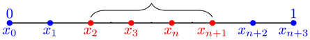
By taking into account the homogeneous boundary conditions and by neglecting the approximation error, we approximate the nodal value with the value of for , where and is the solution of the linear system
for all .
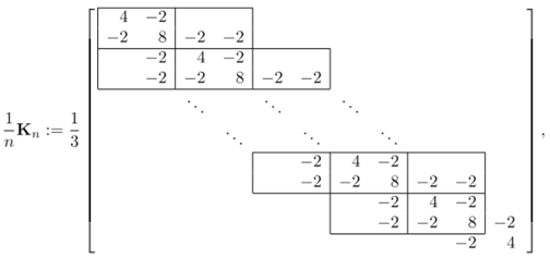
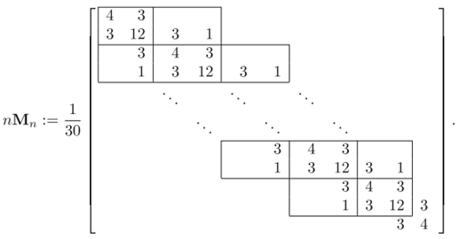
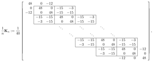
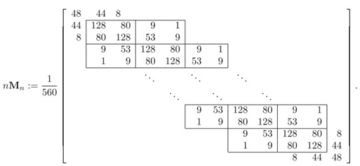
The structure of the resulting matrix is as reported below
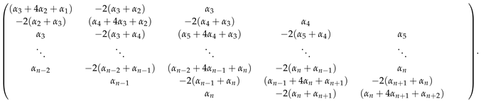
Looking at in (21), we observe that it can be written as
with
It is easy to check that grids and are asymptotically uniform in , according to the notion given in [6]. In fact, for we have
For we have
For we have
Hence, by , part 2, and by [6], we deduce that , and . In conclusion, by invoking , we infer
Eigenvalue Distribution
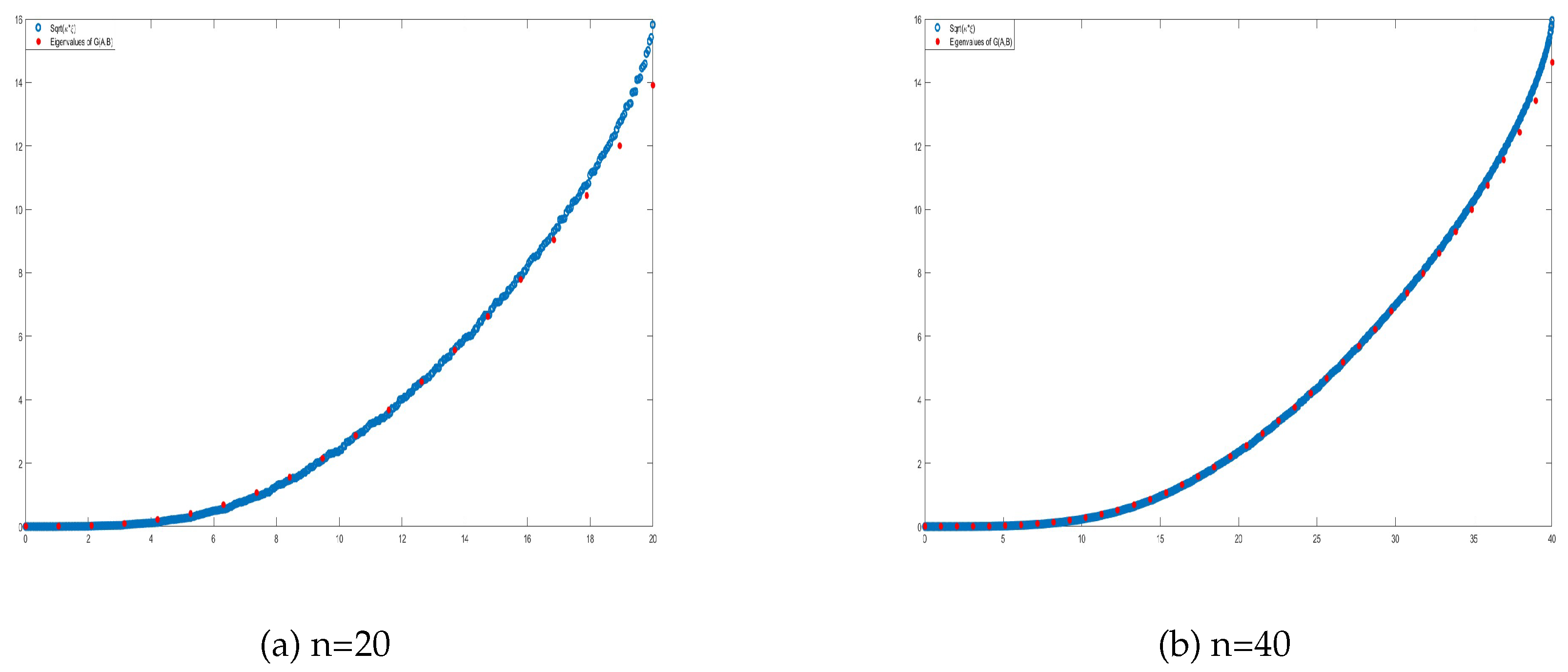
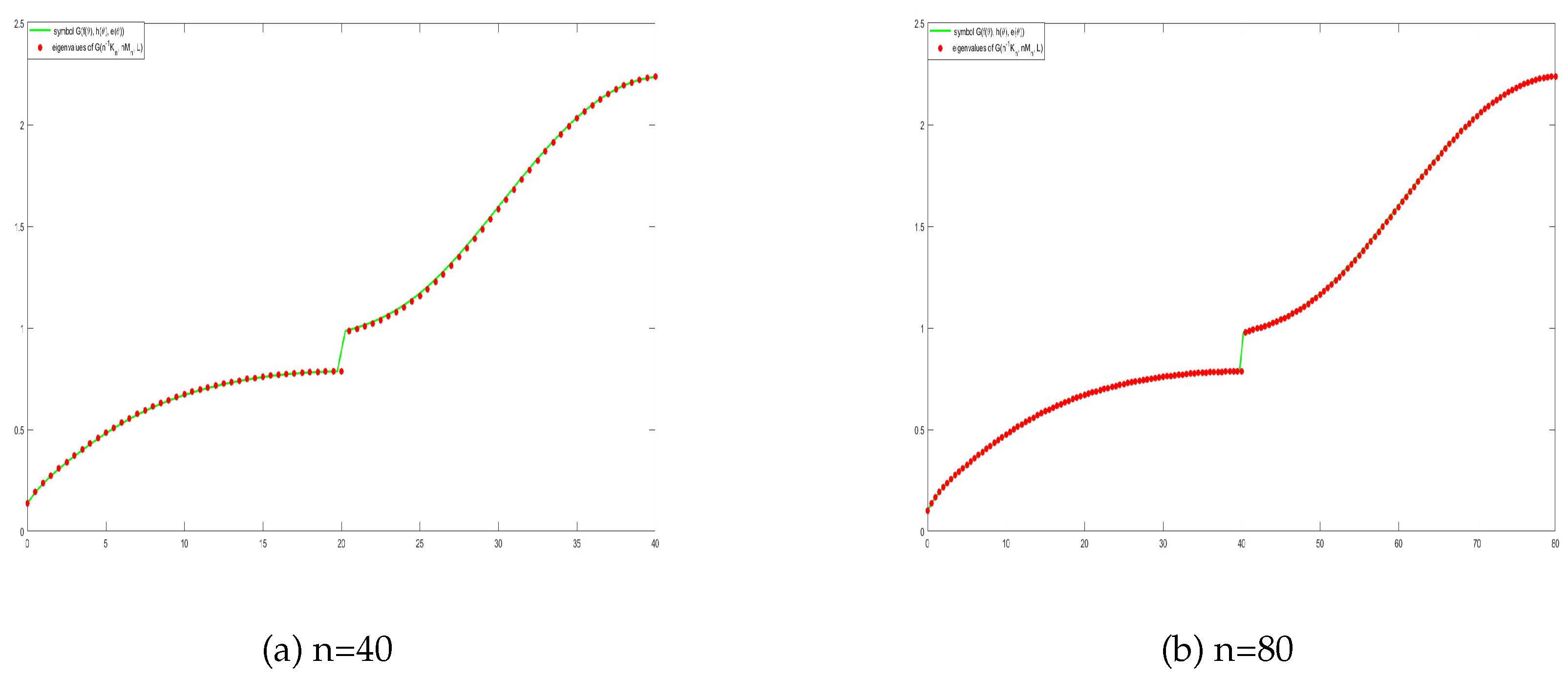
We begin by numerically verifying the eigenvalue distribution of the matrix-sequence with respect to its GLT symbol according to Theorem 8, with , as in (21) with , , . In Figure 1, we compare the eigenvalues of the geometric mean with a uniform sampling of the symbol. It is evident that, as n increases, the symbol provides a better and better approximation of the eigenvalues. Similar results for the two-dimensional case are shown in Example Section 4.2, Figure 2.
Figure 1.
Comparison between the symbol and .
4.2. Example 2 (2D)
Let according to the notation in Section 2.7 with and be the finite difference discretization of the differential operator
on the open domain , with nonnegative on the closure of , with homogeneous Dirichlet boundary conditions on , and zero normal derivatives at .
Regarding , the generating function is given by
with .
Thus, we have
As in the one-dimensional setting in Example Section 4.1, we apply the second-order central finite difference scheme separately to the x- and y-directions, in perfect analogy with the 1D case, and take , . Choosing the related problem is semielliptic, but it is of separable nature. This separable nature is reflected algebraically in a tensor decomposition of the whole approximation and in fact we find that resulting global matrix is given by the Kronecker sum
where denotes the identity matrix of size n and is exactly the structure displayed in (21). By exploiting the GLT analysis in the one-dimensional case, the symbol for the two-dimensional matrix-sequence can be derived similarly. More precisely, we have
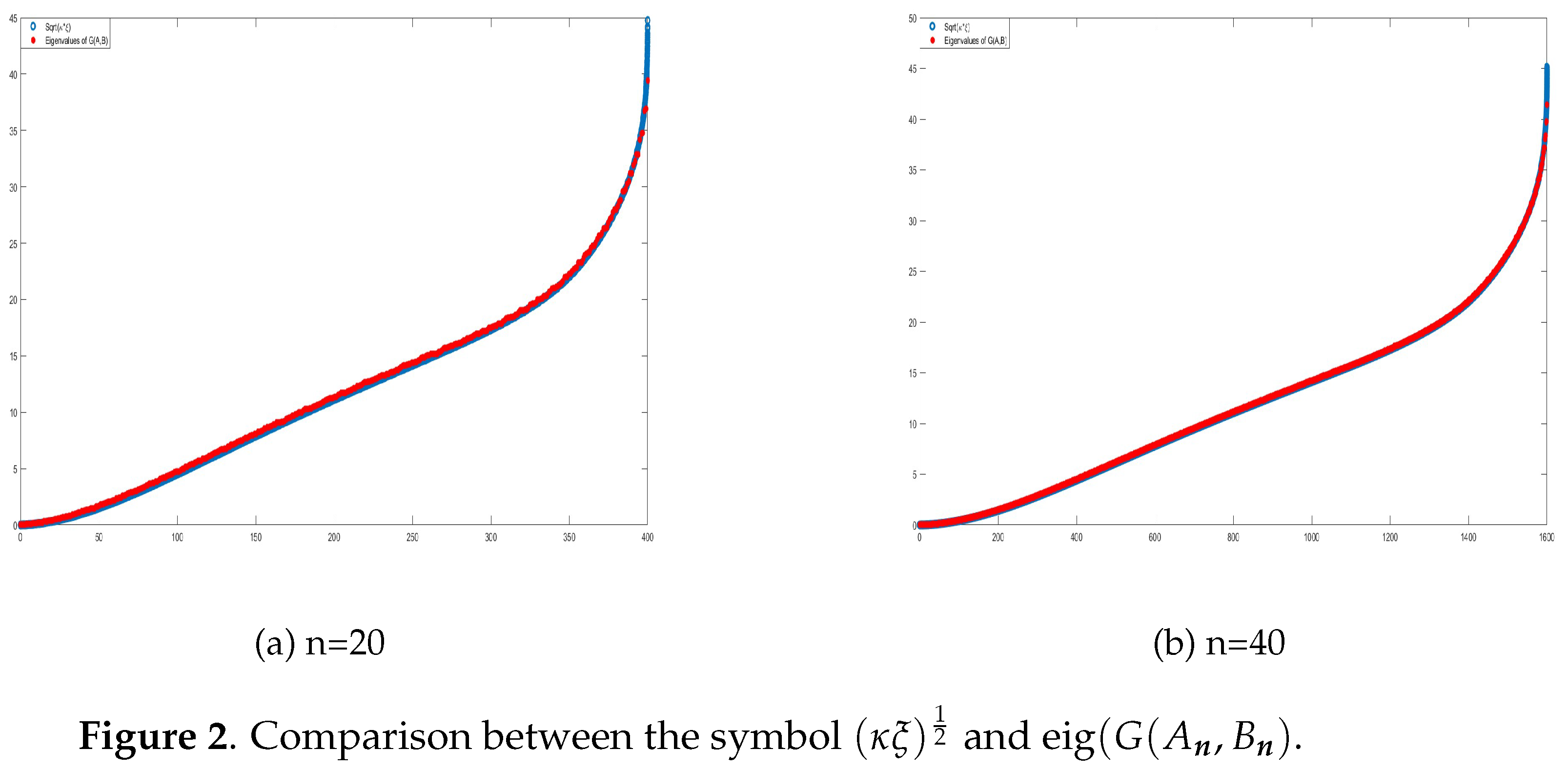
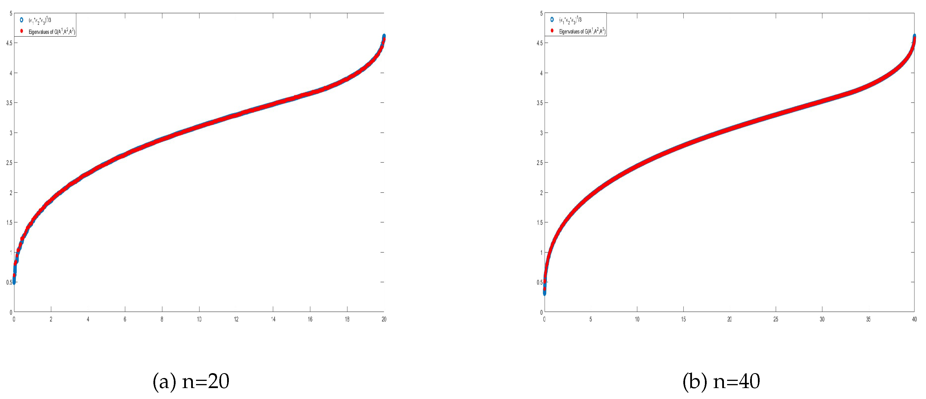
As shown in Figure 2, the agreement is remarkable even for the largest eigenvalues for which the absolute discrepancy is higher.
Figure 2.
Comparison between the symbol and .
4.3. Example 3 (1D)
Let , , and , where is the Toeplitz operator for as in Section 2.7 and is the diagonal matrix generated by the continuous function , according to the notation in Section 2.8.
Eigenvalue distribution
First, we aim to verify the eigenvalue distribution of more than two matrices using the Karcher mean. In Figure 3, we compare the eigenvalues of the Karcher mean with a uniform sampling of the resulting limit GLT symbol. It can be observed that the symbol provides a reliable approximation of the eigenvalues, and in fact, as n increases, the spectral distribution holds asymptotically. Similar results for the two-dimensional case are shown in Example Section 4.4, Figure 4. Both types of result corroborate the conjecture on the GLT nature of the limit matrix-sequence of the Karcher means, as discussed at the end of Section 3.2.
Figure 3.
Comparison between the symbol and .
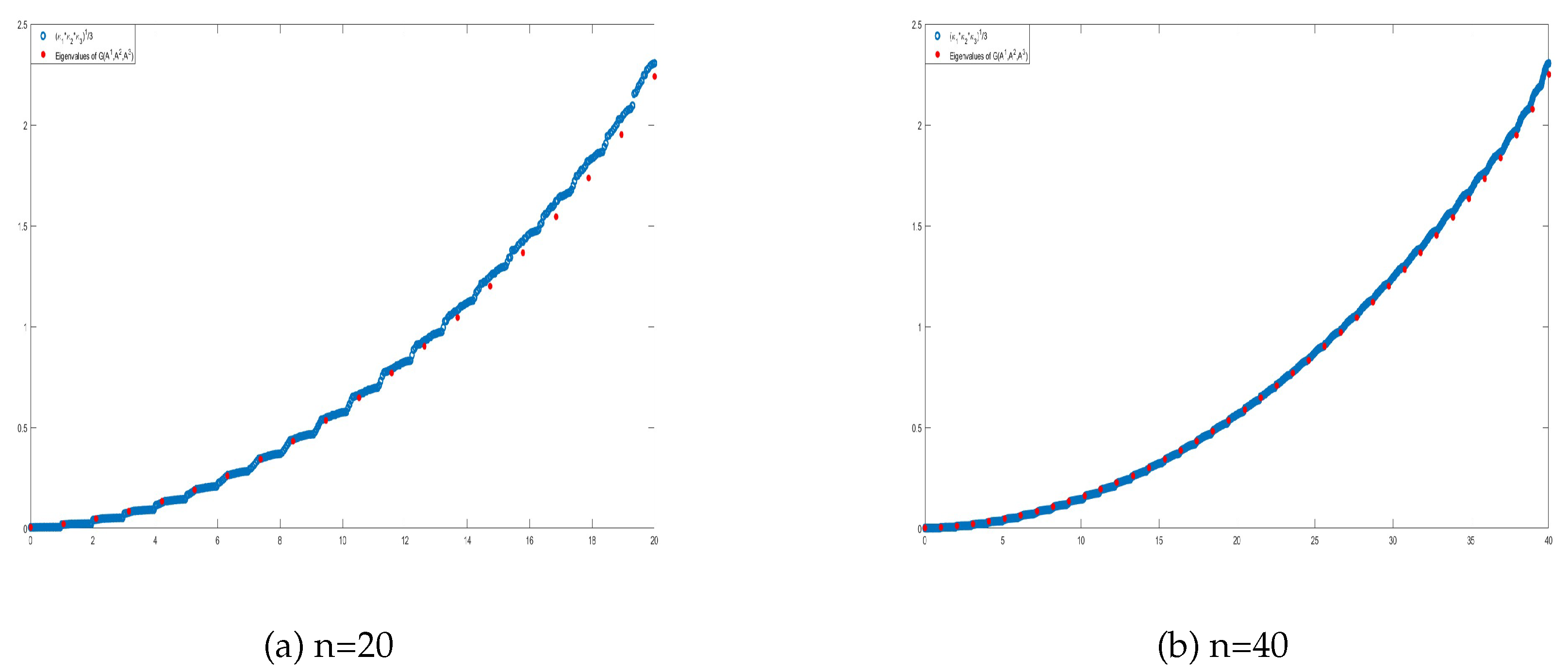
Figure 4.
Comparison between the symbol and .
4.4. Example 4 (2D)
Consider the matrix , where is the Toeplitz operator as in Section 2.7 with , and the function is defined as , with , resulting in .
Also, consider the diagonal matrix , where, according to the notation in Section 2.8, is the diagonal sampling matrix generated by a continuous function , which is positive on the domain .
We take the matrix , where is positive and unbounded on the domain , and where the generating function , with implies that is .
Also in the current example the agreement between the limit GLT symbol and the displayed eigenvalues is remarkably good, so giving ground to the conjecture on the Karcher means reported in the final part of Section 3.2.
4.5. Galerkin Discretization of the Laplacian Eigenvalue Problem
The one-dimensional Laplacian eigenvalue problem is given by the differential equation
with Dirichlet boundary conditions:
The goal is to find the eigenvalues and corresponding eigenfunctions , for , where is the standard Sobolev space of functions with derivatives and vanishing at the boundaries.
Weak formulation
To derive the weak formulation, we multiply both sides of the differential equation by a test function and integrate over the interval i.e. . Using integration by parts on the left-hand side and noting that the boundary terms vanish, we deduce , so that the weak form becomes
for every test function . The latter is rewritten compactly as
where the bilinear form and the inner product are defined as
Galerkin Approximation
The weak formulation allows us to use the Galerkin method to approximate the solution. Let be a finite-dimensional subspace of . The weak problem now becomes: find approximate eigenvalues and eigenfunctions , for such that, for all , we have . By expanding and in terms of the basis functions , we obtain , , and substituting into the bilinear forms, the generalized eigenvalue problem
is defined, where the stiffness matrix and mass matrix are defined as
Both and are symmetric and positive definite, due to the coercive character of the underlying bilinear forms.
4.6. Quadratic C0 B-Spline Discretization
In the quadratic C0 B-spline discretization of the one-dimensional Laplacian eigenvalue problem, the basis functions are chosen as B-splines of degree 2 defined on a uniform mesh with step size . The basis functions are explicitly constructed on the knot sequence (excluding the first and last B-splines, which do not vanish on the boundary of ); see [22]. The resulting normalized stiffness and mass matrices are given by
The stiffness matrix and the mass matrix contain, as principal submatrices, the unilevel 2-block Toeplitz matrices and , according to the notation in Section 2.7 with and , where the generating functions and are given by
and
Since for any Lebesgue integrable generating function g (Axiom GLT 2, part 1), the theory of GLT sequences and a basic use of the extradimensional approach [2,42] lead to
By the Axiom GLT 3, the linear combination of two GLT sequences is again a GLT sequence, with the symbol being the corresponding linear combination of their symbols. The matrix-sequence with
is a linear combination of the sequences and . Consequently,
where and are the symbols of the stiffness matrix and the mass matrix , respectively.
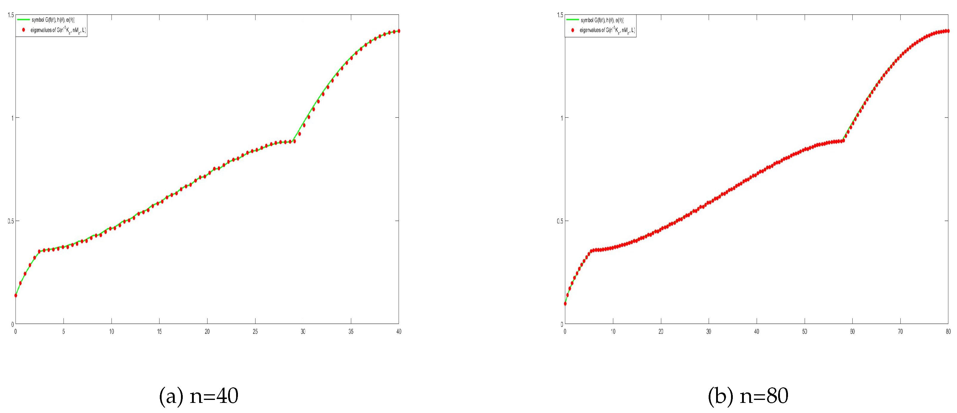
Figure 5.
Comparison between the symbol and .
The numerical evidence is convincing: furthermore, from the related figure, we observe that there exist two branches of the spectrum in accordance with Theorem 5 with .
4.7. Cubic C1 B-Spline Discretization
In the cubic C1 B-spline discretization on a uniform mesh with step size , the basis functions are chosen as the B-splines; see [22]. The resulting normalized stiffness and mass matrices are given by
 According to the notation in Section 2.7 with and , the stiffness matrix and the mass matrix contain, as principal submatrices, the unilevel 2-block Toeplitz matrices and , where the generating functions and are matrix-valued functions given by
and
As discussed in Section 4.6, the same reasoning applies to the matrix-sequence with
which results in the GLT sequence symbol . The numerical evidence is again strong and we can see from the related figure that there exist two branches of the spectrum in accordance with Theorem 5 with .
According to the notation in Section 2.7 with and , the stiffness matrix and the mass matrix contain, as principal submatrices, the unilevel 2-block Toeplitz matrices and , where the generating functions and are matrix-valued functions given by
and
As discussed in Section 4.6, the same reasoning applies to the matrix-sequence with
which results in the GLT sequence symbol . The numerical evidence is again strong and we can see from the related figure that there exist two branches of the spectrum in accordance with Theorem 5 with .
Figure 6.
Comparison between the symbol and .
4.8. Minimal Eigenvalues and Conditioning
In the last part of the current numerical section, we consider the problem of understanding the extremal behavior of the spectral of the conditioning of in dependence of the analytical features of the corresponding GLT symbol. The idea is borrowed from the literature, where we find papers dealing with the extremal eigenvalues in a Toeplitz setting [16,29,30,37], in a r-block Toeplitz setting [31,32], in a differential setting [27,43], including multilevel cases of . Here we restrict our attention to the unilevel scalar setting with and we consider again the examples in Section 4.1 and in Section 4.3.
4.8.1. Example 1 (1D): Minimal Eigenvalue
We consider the example in Section 4.1. The generating function of has a unique zero of order 4 at , while the matrix-sequence shows the GLT symbol with combinations of zeros at of order 1 and at of order 4. According to the theory, the minimal eigenvalue of is positive and tends to zero as (see [16,29,30,37]). On the other hand, according to [27,43], we know that eigenvalue of is positive and tends to zero as . If we consider the geometric mean of the two symbols, we deduce that it has again zeros of order at most 4: as a consequence, heuristically we expect that the minimal eigenvalue of is positive and tends to zero as as it is perfectly verified in the table below with tending to 4.
- Take
- Compute
- Compute

| 0.00010994 | 3.8698 | |
| 0.00000752 | 3.9398 | |
| 0.00000049 | 4.0297 | |
| 0.00000003 |
4.8.2. Example 3 (1D): Minimal Eigenvalue
We consider the example in Section 4.3. The generating function of is strictly positive, the generating function of has a unique zero of order 2 at , while the matrix-sequence shows the GLT symbol with combinations of zeros at of order 4 and at of order 4. According to the theory, the minimal eigenvalue of is positive and tends to as (see [16,29,30,37]). On the other hand, according to [27,43], we know that eigenvalue of is positive and tends to zero as , while for it is trivial tp check that the minimal eigenvalue tends to zero as . If we consider the geometric mean of the two symbols, we observe that it has zeros of order at most 2: hence, heuristically we expect that the minimal eigenvalue of is positive and tends to zero as as it is perfectly verified in the table below with tending to 2.
- Take
- Compute
- Compute
| 0.0014 | 2.2223 | |
| 0.00034797 | 2 | |
| 0.000086993 | 2 | |
| 0.000021748 |
5. Conclusions
We have studied the spectral distribution of the geometric mean of two or more matrix-sequences constituted by HPD matrices, under the assumption that k input matrix-sequences belong to the same d-level, r-block GLT *-algebra, where , . For an explicit formula exists and this has allowed to prove that the new matrix-sequence is of GLT type for any fixed , with GLT symbol being the corresponding geometric mean of the input symbols, according to Theorems 4 and 5. As a consequence the spectral distribution of the geometric mean of matrix-sequences is formally demonstrated. For , an explicit formula is not available and we have considered the Karcher mean, for which efficient iterative procedures available in the literature can be used for computational purposes. Interestingly enough, using the same tools as in the proof of Theorems 4 and 5, we have shown that all the matrix-sequences made by the Karcher mean iterates are still GLT matrix-sequences with symbols converging the geometric mean of the k symbols, provided that the matrix-sequence of the initial input matrices is a GLT matrix-sequence made by HPD matrices. The theoretical results have been confirmed through various numerical experiments, where we compared the eigenvalues of the geometric mean with a uniform sampling of the geometric mean of the symbols. A very good agreement has been observed in all the numerical tests and aven for very moderate matrix-sizes. In fact, as the matrix-size increases, the symbol provides a better and better approximation of the eigenvalues, both in one-dimensional and two-dimensional cases, and both with scalar and block matrices, i.e. using GLT matrix-sequences taken from the differential world with , and including finite difference, finite element, isogeometric analysis approximations of constant and variable differential operators. Few open questions remain and in the subsequent lines we indicate three main issues:
- A formal proof of the GLT nature of the Karcher mean of HPD GLT matrix-sequences has to be given under the assumption that the initial guess is a HPD GLT matrix-sequence; in this respect, also from a computational viewpoint, starting with a initial guess having already as GLT symbol the geometric mean of the input symbols should reduce sensibly the number of iterations;
- in connection with Theorems 4 and 5 and , the ALM axioms suggest that the technical assumption on the invertibility almost everywhere of the input GLT symbols is not necessary for every ;
- a completely open problem concerns the study of the extremal eigenvalues of the geometric means of GLT matrix-sequences as a function of the analytic features of the geometric means of the GLT symbols: in this direction it should be recalled that a rich literature exists regarding the extremal eigenvalues in a Toeplitz setting [16,29,30,37], in a r-block Toeplitz setting [31,32], in a differential setting [27,43], so involving all the types of examples considered in the numerical experiments. Prelinary numerical experiments in the unilevel scalar setting with has been performed in Section 4.8 and the results are quite promising. Interestingly enough, and substantially mimicking the cases already studied in the literature, it seems that the order of the zeros of the GLT symbol decides the asymptotic behavior of the minimal eigenvalues and hence of the conditioning of , at least for , .
All the previous items show that a lot of scientific research has still to be done in connection with the findings discussed in the current work.
References
- T. Ando, C.-K. Li, R. Mathias, Geometric Means, Linear Algebra and its Applications, 385 (2004), pp. 305–334.
- N. Barakitis, P. Ferrari, I. Furci, S. Serra-Capizzano, An extradimensional approach and distributional results for the case of 2 × 2 block Toeplitz structures, Springer Proceedings on Mathematics and Statistics, (2025), in press.
- F. Barbaresco, New foundation of radar Doppler signal processing based on advanced differential geometry of symmetric spaces, in: International Radar Conference 2009, Bordeaux, France, 2009.
- G. Barbarino, Equivalence between GLT sequences and measurable functions, Linear Algebra and its Applications, 529 (2017), pp. 397–412. [CrossRef]
- G. Barbarino, A systematic approach to reduced GLT, BIT 62 (3) (2022), PP. 681–743. [CrossRef]
- G. Barbarino, C. Garoni, An extension of the theory of GLT sequences: sampling on asymptotically uniform grids, Linear and Multilinear Algebra, 71 (12) (2023), pp. 2008–2025. [CrossRef]
- G. Barbarino, C. Garoni, S. Serra-Capizzano, Block generalized locally Toeplitz sequences: theory and applications in the unidimensional case, Electronic Transactions on Numerical Analysis, 53 (2020), pp. 28–112. [CrossRef]
- G. Barbarino, C. Garoni, S. Serra-Capizzano, Block generalized locally Toeplitz sequences: theory and applications in the multidimensional case, Electronic Transactions on Numerical Analysis, 53 (2020), pp. 113–216. [CrossRef]
- R. Bhatia, Matrix Analysis, Graduate Texts in Mathematics, vol. 169, Springer-Verlag, New York, 1997.
- R. Bhatia, Positive Definite Matrices, Princeton University Press, 2007.
- D.A. Bini, B. Iannazzo, The Matrix Means Toolbox, http://bezout.dm.unipi.it/software/mmtoolbox/. Retrieved 7 May 2010.
- D.A. Bini, B. Iannazzo, A note on computing matrix geometric means, Advances in Computational Mathematics, 35 (2–4) (2011), pp. 175–192. [CrossRef]
- D.A. Bini, B. Iannazzo, Computing the Karcher Mean of Symmetric Positive Definite Matrices, Linear Algebra and its Applications, 438 (2013), pp. 1700–1710. [CrossRef]
- D.A Bini, B. Meini, F. Poloni, An effective matrix geometric mean satisfying the Ando-Li-Mathias properties, Math. Comp. 79 (269) (2010), pp. 437–452. [CrossRef]
- S. Bonnabel, R. Sepulchre, Riemannian metric and geometric mean for positive semidefinite matrices of fixed rank, SIAM Journal on Matrix Analysis and Applications, 31 (3) (2009), pp. 1055–1070. [CrossRef]
- A. Böttcher, S.M. Grudsky, On the condition numbers of large semi-definite Toeplitz matrices, Linear Algebra and its Applications, 279 (1-3) (1998), pp. 285–301.
- A. Böttcher, B. Silbermann, Introduction to large truncated Toeplitz matrices, Universitext. Springer-Verlag, New York, 1999.
- P.T. Fletcher, S. Joshi, Riemannian geometry for the statistical analysis of diffusion tensor data, Signal Processing, 87 (2007), pp. 250-262.
- C. Garoni, Topological foundations of an asymptotic approximation theory for sequences of matrices with increasing size, Linear Algebra and its Applications, 513 (2017), pp. 324–341. [CrossRef]
- C. Garoni, S. Serra-Capizzano, Generalized locally Toeplitz sequences: theory and applications. Vol. I, Springer, Cham, 2017.
- C. Garoni, S. Serra-Capizzano, Generalized locally Toeplitz sequences: theory and applications. Vol. II, Springer, Cham, 2018.
- C. Garoni, H. Speleers, S.-E. Ekström, A. Reali, S. Serra-Capizzano, T.J.R. Hughes, Symbol-based analysis of finite element and isogeometric B-spline discretizations of eigenvalue problems: exposition and review, Archives of Computational Methods in Engineering. State of the Art Reviews, 26 (5) (2019), pp. 1639–1690. [CrossRef]
- U. Grenander, G. Szegö, Toeplitz forms and their applications, California Monographs in Mathematical Sciences. University of California Press, Berkeley-Los Angeles, 1958.
- N.J. Higham, Functions of Matrices: Theory and Computation, Society for Industrial and Applied Mathematics, Philadelphia, PA, USA, 2008.
- J.H. Manton, A globally convergent numerical algorithm for computing the centre of mass on compact Lie groups, in: Eighth International Conference on Control, Automation, Robotics and Vision, ICARCV 2004, Kunming, China, 2004.
- M. Moakher, A differential geometric approach to the geometric mean of symmetric positive-definite matrices, SIAM Journal on Matrix Analysis and Applications, 26 (3) (2005), pp. 735–747. [CrossRef]
- D. Noutsos, S. Serra Capizzano, P. Vassalos, The conditioning of FD matrix sequences coming from semi-elliptic differential equations, Linear Algebra and its Applications, 428 (2-3) (2008), pp 600–624. [CrossRef]
- Y. Rathi, O. Michailovich, A. Tannenbaum, Segmenting images on the tensor manifold, in: Proceedings of Computer Vision and Pattern Recognition, 2007, pp. 1-8.
- S. Serra-Capizzano, On the extreme spectral properties of Toeplitz matrices generated by L1 functions with several minima/maxima, BIT, 36 (1) (1996), pp. 135–142.
- S. Serra-Capizzano, On the extreme eigenvalues of Hermitian (block) Toeplitz matrices, Linear Algebra and its Applications, 270 (1998), pp. 109–129.
- S. Serra-Capizzano, Asymptotic results on the spectra of block Toeplitz preconditioned matrices, SIAM Journal on Matrix Analysis and Applications, 20 (1) (1999), pp. 31–44.
- S. Serra-Capizzano, Spectral and computational analysis of block Toeplitz matrices having nonnegative definite matrix-valued generating functions, BIT, 39 (1) (1999), pp. 152–175.
- S. Serra-Capizzano, Distribution results on the algebra generated by Toeplitz sequences: a finite-dimensional approach, Linear Algebra and its Applications, 328 (1-3) (2001), pp. 121–130. [CrossRef]
- S. Serra-Capizzano, Spectral behavior of matrix sequences and discretized boundary value problems, Linear Algebra and its Applications, 337 (2001), pp. 37-78. [CrossRef]
- S. Serra-Capizzano, Generalized locally Toeplitz sequences: spectral analysis and applications to discretized partial differential equations, Linear Algebra and its Applications, 366 (2003), pp. 371–402. [CrossRef]
- S. Serra-Capizzano, The GLT class as a generalized Fourier analysis and applications, Linear Algebra and its Applications, 419 (2006), pp. 180–233. [CrossRef]
- S. Serra-Capizzano, P. Tilli, Extreme singular values and eigenvalues of non-Hermitian block Toeplitz matrices, Journal of Computational and Applied Mathematics, 108 (1-2) (1999), pp. 113–130. [CrossRef]
- P. Tilli, Locally Toeplitz sequences: spectral properties and applications, Linear Algebra and its Applications, 278 (1998), pp. 91–120.
- P. Tilli, A note on the spectral distribution of Toeplitz matrices, Linear and Multilinear Algebra, 45 (2-3) (1998), pp. 147–159.
- C.A. Tracy, H. Widom, Level-spacing distributions and the Airy kernel, Communications in Mathematical Physics, 159 (1) (1994), pp. 151–174.
- E.E. Tyrtyshnikov, A unifying approach to some old and new theorems on distribution and clustering, Linear Algebra and its Applications, 232 (1996), pp. 1–43.
- E.E. Tyrtyshnikov, Extra dimension approach to Spectral Distributions, Private discussion (1997).
- P. Vassalos, Asymptotic results on the condition number of FD matrices approximating semi-elliptic PDEs, Electronic Journal of Linear Algebra, 34 (2018), pp. 566-581.
Disclaimer/Publisher’s Note: The statements, opinions and data contained in all publications are solely those of the individual author(s) and contributor(s) and not of MDPI and/or the editor(s). MDPI and/or the editor(s) disclaim responsibility for any injury to people or property resulting from any ideas, methods, instructions or products referred to in the content. |
© 2024 by the authors. Licensee MDPI, Basel, Switzerland. This article is an open access article distributed under the terms and conditions of the Creative Commons Attribution (CC BY) license (http://creativecommons.org/licenses/by/4.0/).
Copyright: This open access article is published under a Creative Commons CC BY 4.0 license, which permit the free download, distribution, and reuse, provided that the author and preprint are cited in any reuse.


