Submitted:
17 December 2024
Posted:
18 December 2024
You are already at the latest version
Abstract
This paper presents a machine learning-based approach to grade engine health and generate a respective score ranging from 0 to 100 for tuned high-performance vehicles. It integrates the technical intricacies of automotive engineering with machine learning practices in a clear and sequential process. Data is collected from sensors monitoring RPM, boost, rail pressure, timing, and temperature. The data is processed for supervised learning and analyzed using scatter, pair, heatmap, PCA, parallel coordinates, and t-SNE plots. Models are trained, innovatively tuned through hyperparameter optimization, and tested for their ability to grade new data logs. Results highlight K-Neighbors, Extra Trees, and Extreme Gradient Boosting as exceptional regressors for this task, with Gradient Boosting, Support Vector Machine, and Random Forest trailing behind. This automated grading of engine health and performance enhances objectivity and efficiency in the tuning process, and potentially serves as a basis for a digital twin. The developed methodology is discussed in the context of health evaluation for any sensor-based system, with practical applications extending across various domains and industries.
Keywords:
automotive
; engine
; hyperparameter
; logs
; machine learning
; sensors
; tuning
; visualization
1. Introduction
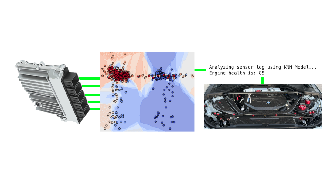
Tuning the engine of a car refers to modifying the default parameters in its Engine Control Unit (ECU), often to extract performance [1]. The ECU is a computer module located in the engine bay of the vehicle that manages and controls various aspects of the engine [2]. It does this by reading sensor data, performing the necessary calculations, and then sending signals to the different components in the car. The traditional method of monitoring the car and engine through the use of error codes and regular maintenance is acceptable for stock vehicles as the manufacturer has done extensive testing, but is not adequate for tuned vehicles as different parameters are used [3].
Tuners use a notion known as logging to verify their work. Logging refers to collecting a data log of various sensor values. Through post analysis of a log, a tuner can receive feedback on how the engine and supporting parts operated, and adjust parameters as needed.
Our main goal in this research is to create a model that is able to read a log and tell us if the engine is functioning optimally. We will do this using a method that involves collecting, processing, and analyzing sensor data, and then using it to train, validate, and test machine learning models. Success in automating the task of log grading makes the tuning process more objective and efficient [4], and as will be discussed, is crucial for the performance and reliability of the engine. In addition, the methodical process shown here can be applied to extend the scope of machine learning in tuning applications and also used to monitor the health of any system containing sensors.
2. Materials
2.1. Test Vehicle
The car that is used in this research is of a BMW make. The platform that is used for the tuning tasks is known as MHD, which is a popular tuning solution. MHD allows flashing of maps, which are files containing various ECU parameters and codes. MHD allows for the flashing of three different types of maps: OEM, OTS, and custom [5]. The OEM map is the file that all cars of the same make come with from the manufacturer. The second is known as off-the-shelf, and is a full remap of the parameters, and is created and provided by the tuning platform themselves, in this case MHD. The third is a map that a tuner has created specifically for an individual vehicle. We will be using an OTS map, as it is the most generic tuned map that is available. An OTS map is not car specific, but rather engine specific. Any car equipped with the engine that the OTS map was designed for can accept the OTS map into its ECU. The OTS maps are named in stages, such as Stage 1, which is flashed onto an otherwise stock vehicle. By stock vehicle we refer to a car that has very minimal modifications done to it regarding the engine and the supporting components. Stage 2, which is the map on the test vehicle, requires an aftermarket high-flow downpipe, which is a pipe that is connected to the turbo and responsible for directing the gasses from the combustion process out and away from the engine bay. The factory downpipe that comes with the vehicle by default has a restrictive catalytic converter, which limits airflow, and thus parameters that an engine tune can run [6]. While the models in this research will be trained with data mostly gathered from one configuration of car, the only requirement to use our model on a similar car is to simply log the same sensors. The methodology otherwise remains the same and can be used to create models for any vehicle or system.
2.2. Engine
The engine in the test vehicle is the second generation B58, also codenamed B58TU. This is one of the most popular engines in which tuning is performed upon at the moment. The B58 is fed from a single turbocharger, often shortened to turbo. A turbo increases an engine’s power output by forcing more air into the combustion chamber. This is done by drawing in air and compressing it. The increased air leads to higher power than an equivalent naturally aspirated engine would produce [7]. Tuning is most often performed on vehicles with a turbocharger, as one of the biggest elements in the tuning process is increasing boost levels, which is the pressure of the compressed air.
3. Data Collection
3.1. Logging
MHD has logging capabilities, where data logs are collected by connecting a smartphone to a dongle attached to the OBD port on the car. Through the MHD app, the sensors that a user wishes to monitor are selected. There are over 700 sensors available using this method. Our goal is to select the most important sensors. We want relevant, high-quality, and non-redundant information to get good results.
3.2. Attribute Selection
The features that we choose to focus on are: Acceleration Pedal Position, RPM, Boost Level, Rail Pressure, Timing, and Intake Temperature.
3.3. Procedure
The data that is collected is during what is known as a pull. A pull is a controlled test in which the car is accelerated under specific conditions. The pull is conducted at wide-open throttle (WOT), which means the accelerator pedal is pushed down to its maximum position, or 100 percent, requesting the maximum amount of power from the vehicle. The pull ranges from the lowest possible RPM to the highest possible RPM (also known as redline). This is done in a specific gear, and is usually the same gear that is used on dynamometers, which is a device that can measure the power output of a vehicle. This gear is generally the one that gives a 1:1 gear ratio; or the gear that is one lower or one higher than it. For vehicles with the B58 engine containing the ZF8 automatic transmission and associated gearbox, this is 5th gear, but 4th gear is often used instead [8]. Executing the pull in a lower gear such as first results in erratic readings as the vehicle goes through the gear and RPM range too quickly. In addition, the chance of wheel spin in a lower gear is greater, due to inertia and torque multiplication. Conversely, doing a pull in a higher gear such as 6th imposes more of a safety risk due to greater speeds, and more of the RPM range is wasted from lugging the engine. The data was collected using the following method: shift manually into 4th gear, drop the RPMs to around 2000, and floor the pedal until the rev limiter kicks in. This was and should be carried out on a straight road with safety precautions.
3.4. Example Pull
An example of the data collected during a pull can be seen in Figure 1. The data logs are saved as comma-separated values (.csv files) and can be visualized. A popular website used by tuners for doing so is known as Datazap [9]. In the figure we can see how the values change over the pull. The gray line at the top is the acceleration pedal position. We can see that it goes from 0 to 100 nearly instantly as we floor the pedal. The dark gray line towards the center that climbs throughout the pull is RPM. The orange line represents boost deviation, which is at a maximum during the acceleration pedal transition from 0 to 100, as the ECU requests a high boost pressure. The time that it takes for the boost deviation to stabilize is known as turbo lag. We can see the intake temperatures in the ivory color rise during the pull, as the turbo heats up and starts blowing hotter air. The timing corrections throughout the pull for each cylinder are 0, so they are all on the same line as the purple one. The rail pressure deviation is the light gray sawtooth-like wave near the center. The variance is in an acceptable range and there are no large negative spikes. We can see that as the RPMs approach 7000 or redline, the readings become erratic, as the rev limiter cuts power to prevent over-revving the engine. The jargon used here will be explained shortly.
3.5. Sample Size
In a single pull, which will correspond to one data log, there are approximately 100 rows of data. Each row contains readings from all the selected sensors at that moment in time. The number of rows in a pull depends on several factors including the power of the car and the sample rate of the logger. An aggressively tuned car will go through the pull quicker than a moderately tuned car will, and a faster logger will capture more samples in a period of time than a slower one. Shorter and longer gear ratios on different gearboxes will have an effect as well. While 100 rows per pull does not seem like a large amount of data, the number of rows is not as important as the quality of the data log. A quality data log reflects what happened during the pull, whether it has 50 or 500 rows. The diversity of the data logs we can collect is far more crucial. We want a dataset with a high variance.
As an experiment, a data log over an entire 20-minute drive was recorded. This data file contained tens of thousands of rows. The issue now however was that there was no longer a baseline of 100% acceleration pedal position. As a result, a model capable of discerning patterns over varying vehicle loads would have to be developed, since most of data was at less than 100% throttle. A model trained on such data would be less effective at accurately predicting health scores of 100% throttle pulls, which is a pitfall for our goal, as idle and low-load situations contain little useful information regarding performance. If a model was being developed to instead analyze the efficiency of a car’s engine, then this approach could prove insightful, but otherwise ends up adding a considerable amount of noise to our data.
3.6. Feature Overview
We briefly mentioned the information collected. Let us go over the concepts and then we can discuss the actual sensors chosen.
3.6.1. RPM
Revolutions Per Minute is the number of rotations that the crankshaft, which converts the linear motion of the pistons into rotational motion to power the drivetrain, undergoes [10]. RPM is chosen because it gives the machine learning model context on all the other values. Each row in our data has an associated RPM, and so the model knows at which RPM those values occurred at. This is crucial because in the learning we perform, the model must be able to differentiate between values that occurred at low RPMs, high RPMs, and everything in between.
3.6.2. Boost
Boost is a term that refers to the air pressure at the location of the respective air sensor. Fresh air is drawn through the front grille of the car into the intake system, which routes the air through a filter to remove debris. The air then enters the turbocharger, whose turbine is spun from the exhaust gasses of the internal combustion process. The turbine drives a compressor which pressurizes the incoming air. This pressurized air travels through the engine bay in what is known as the charge pipe, and enters the intercooler, which is integrated into the intake manifold. The air-to-water intercooler significantly reduces the temperature of the pressurized air, which becomes hot after being compressed. The intercooler can reduce the charged-air temperature by 200 degrees Fahrenheit as observed. This cooled air is eventually fed into the cylinders through the intake manifold. There is a sensor that measures the pressure before the intake manifold, and one that measures it inside. The one inside generally has a 1 PSI lower reading than the one before due to the cooling and physical resistance of the core [11], even though the system as a whole can be thought of as closed [12]. The important thing is that the readings are fully correlated, which is indeed the case, as fluctuations in one part of the system are reflected in the other, and hence either sensor can be used.
3.6.3. Rail Pressure
Similar to boost, rail pressure refers to the pressure of the fuel rather than the air. The rail pressure reading in our data is specific to the high-pressure-fuel-pump (HPFP), which is responsible for delivering fuel to the engine’s fuel injectors in a direct-injection fueling system, which the B58TU uses from factory.
3.6.4. Timing
3.6.5. Intake Air Temperature
Also shortened to IAT, the intake air temperature is the temperature of the air that is entering the intake manifold. It is measured after the intercooler. The temperature between the turbocharger and intercooler, which is the air inside the charge pipe, is the charged-air temperature. The air before the turbocharger is simply the ambient air temperature. The IAT is the most important of the three because it is a measure of the air that enters the cylinder and is used in the combustion process.
3.6.6. Acceleration Pedal Position
A measure of the throttle input provided by the driver, and reflects the power that is being requested from the car. A 100% pedal position represents maximum load and stress.
3.7. Sensor Selection
The above is a list of the information we want to capture. Now we can talk about the sensors that are available to do so.
3.7.1. Boost Sensors
For boost, there are a few sensor options that can be logged. They include Boost Actual, Boost Manifold, Boost Target, and Boost Deviation. Boost Actual is the pressure of the air after it has been compressed by the turbocharger, which as mentioned is known as the charged-air. Boost Manifold is the pressure of the air inside the intake manifold that will enter the combustion chamber, and as noted, is slightly lower than Boost Actual. Boost Target is the pressure that the ECU is requesting. The pressure is controlled by the waste gate, which is a flap located in the turbo housing that opens and closes to allow more pressure to build [15]. If Boost Actual is lower than Boost Target, then the waste gate closes. If Boost Actual is higher than Boost Target, or within a specified tolerance, then the waste gate opens. The operation of the waste gate is controlled by the waste gate duty cycle, and the closer it is to 100, the more closed it is. During the start of the pull, the waste gate is fully open as no power is being requested. When the pedal is floored, the waste gate fully closes to allow Boost Actual to reach Boost Target as fast as possible to minimize turbo lag. When Boost Target is reached, the waste gate duty cycle starts to hover between 80 and 90%. In the case of a leak in the system, the waste gate duty cycle will be 100% throughout the entire pull, as Boost Actual never reaches Boost Target, and the ECU keeps the waste gate closed in a futile attempt to allow the turbo to build the desired pressure. The reason the waste gate opens slightly when the target is reached is to limit the amount of pressure that is generated. The turbocharger can indeed generate more boost, and provide more power, which is essentially what tuning does, but after exceeding a certain pressure, the turbo becomes less efficient and results in less power for the engine as it starts blowing hotter air. Furthermore, the charge pipe, intake manifold, and engine have limits, and over pressure may cause cracks.
Instead of logging the whole slew of these sensors, we can combine the most useful information into one. Boost Deviation is the difference between Boost Target and Boost Actual. If the target is higher than the actual, the boost deviation is positive, and negative if lower. In Figure 1, we can see that during the first moment of the pull, Boost Deviation is at a maximum, as the target is 20 PSI and the actual is 0 PSI. As we follow the orange line, we can see its magnitude drop, as the turbocharger is working to build boost. In a couple hundred RPM, boost deviation has a mean of around 0, meaning that the turbo has spooled. A smaller turbo spools faster than a larger turbo, due to greater pressure differentials throughout the system, but in general, a properly sized turbo should spool within 500-1500 RPM above the starting RPM of the pull. If for example, a pull is initiated at 2300 RPM, and at 5000 RPM the boost deviation is still high, then it is evidence of a problem, such as a leak in the system, damaged turbo, or a malfunctioning waste gate. We want to monitor this, and logging Boost Deviation does just that, and reduces the dimensionality of our dataset [16].
It is also important to mention that we will be focusing on positive boost deviations. It is perfectly normal for the boost deviation to be slightly negative, meaning the actual pressure is higher than the target, as cars are non-perfect machines operating in non-perfect conditions. A pressure deviation ranging from -1 to 1 shows that the tune and car are operating correctly to control boost. We will not focus on large negative boost deviations (overboosts). This will occur and show up in logs, but only after the driver lets off the throttle after the car has already built boost. This is because the pressure vacuum is broken and some of the air forced out through the intake system, creating a surge at the sensor. This scenario only occurs under normal conditions when the acceleration pedal position is below 100%, and as will be shown in a future section, will be discarded. If the car is heavily overboosted for an extended period of time, then the pressure will either destroy the turbo, engine, or interconnecting components. Therefore, predicting the health score of a car that just suffered a catastrophic failure is unnecessary.
3.7.2. Rail Pressure Sensors
The exact same rationale to choose Boost Deviation is used to choose Rail Pressure Deviation, and saves us a feature. Here however, Rail Pressure Deviation is the difference between the Actual Rail Pressure and Target Rail Pressure (opposite of Boost Deviation). Hence, a positive deviation means the HPFP is delivering too much fuel, and a negative deviation means it is not delivering enough. The deviation is reported in terms of MPa in the logs, but is often talked about in units of PSI. A deviation of about -100 to +100 PSI is normal for the HPFP. Large positive values do not occur as the HPFP is a mechanical device capable of only generating a certain amount of pressure. Large negative values however are indicative of a weak HPFP. When the rail pressure goes negative, by more than a few couple hundred PSI, it means that the ECU and tune is requesting more fuel than the pump can provide, and is known as HPFP tanking. Eventually, if negative enough, the rail pressure will crash and power must be pulled to avoid damage to the engine [17]. The HPFP is a robust piece of hardware, and rail pressure tanks and crashes are usually not due to a mechanical failure.
Instead, dips in rail pressures are more commonly caused by the fuel contents. Gasoline is often used to fuel cars, but in high performance tuned vehicles, including the car used in this paper, ethanol is used. Ethanol has a higher octane rating than gasoline, which increases its resilience to premature ignition, also known as knock [18]. This is an issue in higher compression engines like the B58TU, which has a compression rating of 11:1 [8]. Ethanol however has a lower (by 30%) energy content per unit of volume compared to gasoline [19]. This means to produce the same power, 30% more fuel has to be used. This is just the base figure on a stock car. If tuned, then the car must consume even more fuel to produce the additional power over the OEM map. This makes the HPFP work harder, and eventually, will cause rail pressure to tank if it cannot provide the requested amount of fuel. On the B58TU with the factory HPFP, this occurs at around 50% ethanol mix. An ethanol mix is part ethanol and part gasoline. A 50% ethanol mix means that for a 10 gallon fuel tank, 5 gallons are pure ethanol and 5 gallons are pure gasoline. Since E85 pumps contain a varying amount of gasoline, and gasoline pumps contain a varying amount of ethanol, the fuel content has to be analyzed to reach a desired mix. To produce the maximum amount of power from the B58TU engine on the factory HPFP, a 40% (approximately) ethanol mix is used. As the user deviates from this value, power is reduced, and if too high of an ethanol mix is used, such as filling the tank with only ethanol, then the rail pressure will drop. The remedy for this is to upgrade the HPFP to a stronger one, use a different fueling system such as port injection, or simply run a lower ethanol content.
3.7.3. Timing Sensors
The sensors that are associated with timing are for the majority on a per-cylinder basis. The B58 engine is an inline-six engine, meaning there are six cylinders in total arranged in a straight row. There are six sensors, labeled Timing Cyl. 1, Timing Cyl. 2, etc. These are the raw values that the ECU is targeting. They are predetermined and programmed into the map, and are one of the parameters that are modified when tuning a vehicle [20]. They are important to monitor to get a sense of the performance that the tune is targeting, but also to see timing pull and timing advances. Timing pull signifies that the ECU is firing the spark plug later, and timing advance means that it is firing it earlier. Timing pull is the ECU’s response to potential knocking. There exists a dedicated sensor for knock detection, which triggers from dangerous abnormal vibrations of the engine. The most common cause of knock in a tuned vehicle is low quality fuel. Lower-octane fuel is more prone to knock due to early detonation. If the ECU detects knock, it will pull timing to prevent damage to the engine [18]. This delayed firing results in a loss of performance. Generally speaking, up to 3 degrees of timing pull is considered acceptable on a cylinder. Raising the octane level of the fuel in the tank by using higher quality pump gas such as 93 octane (AKI) instead of 91 octane (AKI), or using a higher ethanol mix usually gets rid of these timing pulls. If the values are greater however, then it is a potential concern. If there is significant timing pull on a cylinder, then it could suggest a spark plug or coil pack failure.
It is also important to mention that timing pull at higher RPMs is more serious than at lower RPMs. This is because the shorter combustion duration at higher RPMs lowers the likelihood of knock, and hence knock at high RPMs is more of a concern. Furthermore, the engine is at a high mechanical load at higher RPMs and timing pull means the engine is struggling to maintain safe operation under the most dangerous period [18].
Timing advance on the other hand is considered a pre-calculated value and is already applied in the map to improve performance. Hence in logs, timing advance alone is not generally reported, only the raw timing value itself.
Instead of logging the actual timing values, we will log the timing corrections, consisting of a total of six sensors. The timing corrections show the timing pull on each individual cylinder and are reported in negative degrees in increments of 0.3. The concern here is that we are adding six additional features into our model. To avoid curse of dimensionality, we will employ feature engineering, and simply take the sum of all the timing corrections across all six cylinders. As an example, if at 3500 RPM, Cyl 3’s timing correction was -1.5, Cyl 6’s timing correction was -3, and the rest of the cylinders had zero timing pull, then the total timing correction will be -4.5 for that data row.
3.7.4. RPM, Intake Air Temperature, Acceleration Pedal Position Sensors
For RPM and IAT, we will use the direct sensor values with no modifications.
Acceleration pedal position will be used to clean up our logs and prepare them for training, but will not be used in the learning itself, as it is a redundant feature since every data row in the dataset will have a corresponding acceleration pedal position of 100%, as we are only interested in data from a WOT pull.
4. Data Wrangling
The information collected must be pre-processed before using it as input. Python 3 inside a Jupyter notebook is used for all future programming related tasks throughout this paper.
4.1. Cleaning
An example of an uncleaned data log is shown in Figure 2. We start by removing the first four rows as they contain irrelevant information. Next we remove any columns containing unused features. These include Time, Amb. Pressure, Ethanol Contents, and the last column. These are columns that cannot be disabled in the logger and are always recorded for the user’s information. The starting and stopping of the log recording is done manually by the user while driving, so the log contains data before and after the pull that must be removed. We filter the data by removing any data outside of a WOT condition, or in other words, keep only the rows that have a 100 in the Accel Ped. Pos. (%) column. Next, another filter is applied to keep only values between the 2300 and 6800 RPM range. The pulls are done in 4th gear, which can be manually selected as long as the RPM is above 1500, at which point the automatic transmission will override and downshift to 3rd gear. Our pull is initiated below 2300 RPM, but we only use the values above 2300 RPM to avoid any potential issues that can occur at the start of the pull such as traction loss, which will skew the data. The stock redline of the B58 engine is 7000 RPM, but we exclude any data above 6800 RPM as the chance of running into erratic data above this figure increases drastically as we approach the rev limiter. Next, we sum the six individual timing correction columns into a single column which we name Total Negative Timing Correction. We then reorder the columns from left to right as Accel Ped. Pos. (%), RPM (rpm), Boost deviation (PSI), Rail pressure dev. (MPa), Total Negative Timing Correction, and IAT (°C). We keep the first column, even though it will not be used in the learning, to verify the data after cleaning it and make sure everything is correct.
4.2. Grading
The final task is to label the log, as we will be performing supervised learning.
4.2.1. Procedure
A health score is assigned to each data log. The log as a whole is analyzed, and every row in the log is given an equal health score corresponding to the health of that log. If a certain log has ideal values across the pull, a high health score is assigned. If the values are mediocre, then a medium health score is assigned, and if the values are poor, a low health score is assigned. The reason for this is that we want our model to capture patterns across all features and all rows, and not just individual ones. Essentially, we want our model to learn what a log is. The caveat of doing so however is that we need a very diverse set of logs in order for our model to generalize well to different test data. This is because the information is compacted. If we train our model using a couple of high health logs, it will not predict the score of other health logs. In reality, as we found, it is even poor at predicting the health of other high score logs.
The health score that we assign to the data ranges from 0 to 100. A health score of 0 implies the car essentially does not operate, and a score of 100 represents a perfect car. Generally speaking, high health score files included ideal values in all features, medium health score files included poor values in one feature, and low health score files contained poor values across multiple features. Additionally, there was variance within the same figurative health categories. For example, the file with a health score of 80 had slightly worse values than the file with a health score of 90, even though neither are classified by us as being low health.
4.2.2. Dataset
The training data consisted of 15 individual logs. The file names given to our logs are their respective health scores. They will be described below.
- 94.csv: This file has the highest health score in our dataset. Across the pull, it features boost and rail pressure deviations with a mean of 0, 0 total negative timing corrections, and IATs that start at 43, go down to 40 during the middle of the pull, and rise to 46 towards the end of the pull. These are all ideal figures and reflective of a very optimized tune running on a well functioning vehicle with high fuel quality under good conditions.
- 92.csv: Very similar to 94.csv, but has slightly lower IATs but slightly more boost deviation. All figures are still well within ideal ranges.
- 83.csv: Similar in values to 92.csv, but has higher IATs, starting at 56 and ending at 63. This file represents a good tune, good car, but simply high ambient temperatures, which is unfortunate. We label this with a lower health score as it implies that upgrading the intake manifold with one that features a stronger air-to-water intercooler could lead to improved performance and reliability.
- 80.csv: Very similar in values to 92.csv, but has small negative timing corrections from 2300 to 4300 RPM. The values start at -1.5 and drop to -0.3 towards the end. This shows that the timing pull is both very marginal to begin with and dies off as we approach redline. This is an indication of a small performance loss due to non ideal conditions.
- 73.csv: Like 80.csv but with stronger timing pull in a similar RPM range. It again dies off, this time at 4400 RPM, but starts at -3. This is generally due to using or mixing a low quality pump fuel such as 91 octane (AKI).
- 70.csv: Similar to the timing pull in 80 and 73, but occuring at a higher RPM range, in this case from 6000 to the end of the pull.
- 65.csv: This file, partially shown in Figure 3 has timing pull from 2400 to 5000RPM. It starts at -3, goes to -5.7 in the mid range, and then dies off towards the high. While it occurs in a lower RPM range than 70.csv, it is more severe in magnitude, and overall worse for performance as it happens throughout a larger duration of the pull.
- 60.csv: This file does not have any timing corrections, but has rail pressure deviations. Starting at about 3000 RPM we see a dip of -1 MPa, which is more than expected. The pressure continues to decrease until it reaches a maximum negative value of around -5 MPa, which is equivalent to a drop of 700 PSI. If the target rail pressure in this scenario was 5100 PSI (usual for B58TU), then the actual rail pressure at its worse is about 4400 PSI. This means that the HPFP is struggling to provide the fuel requested and that the engine is running lean, meaning the air-fuel ratio is not optimal. However, the rail pressure in this scenario would not necessarily be deemed crashed, just tanked. The rail pressure deviation stabilizes and goes back up to a mean of 0 when the RPMs reach roughly 4600. The RPM range in which this occurred is considered the mid range, and is where the most torque is generated by the engine, so it is detrimental to performance. The ethanol mix should be slightly lowered in this scenario, as an example.
- 50.csv: Here, the rail pressure deviation is more severe, and occurs from the start of the pull all the way to the end of the pull, averaging about -7 MPa. This is indicative of a crashed HPFP which cannot recover. There are also slight timing corrections during the low-mid range. This file commonly represents a car running a very high ethanol mix on a map designed for a lower one.
- 45.csv: This file represents an overheated system, in which IATs start at 68 and end at 75. Both of these values are over the 150 degree Fahrenheit mark which is considered the maximum value for IAT for the B58 before the ECU starts cutting power. This scenario can happen during a track session in hot climates. The car should be cooled down. A potential fix to extract the maximum performance is to upgrade the cooling components, such as the intercooler and heat exchangers, or to run a higher ethanol mix, which has lower combustion temperatures.
- 40.csv: Timing pull across multiple cylinders throughout the pull. Most commonly due to very low quality fuel.
- 30.csv: Timing corrections across the pull and tanking HPFP. Indicative of a very aggressive tune. Parameters should be dialed back.
- 25.csv: Similar to 30.csv but more severe timing corrections. This tune should not be run to prevent damage to the engine.
- 20.csv: Here we have a boost deviation throughout the pull centered around a mean of 5 PSI. This is fine during the turbo lag stage, but should not occur over the pull. This is indicative that the turbo is not spooling optimally and that there is likely a leak somewhere in the system.
- 15.csv: This is the file with the lowest health score that will be used in training. It is a combination of 20.csv and 25.csv with slightly more severe values.
4.3. Source of Data
All the files ranging from a health score of 40 to 93 were generated from logs collected using the test vehicle. These were done using varying conditions and fuel mixes, which were experimented with using an ethanol content analyzer installed in the low pressure fuel line, which shows the ethanol percentage of the fuel. The lower health score files, ranging from 15 to 30, were collected from publicly available logs from the same B58 engine. This was to avoid damaging the test car when valid data was already available. An adequate dataset should allow for patterns to be recognized and for our models to generalize well to test data. If additional sensors or features are added at a later time, the sample size should be increased.
5. Data Analysis
Running analytics on the data helps validate the decisions made thus far. Additionally, it can give us foresight into how to go about implementing the machine learning and help visualize our greater than 3 dimensional data. Furthermore, this stage can be revisited after the machine learning is performed to better understand the results, and even improve generalization by adding more data, as long as the proper steps to avoid data-leakage are taken.
5.1. Visualization
To illustrate the data from all the files, a matplotlib 3D scatter plot [21] as shown in Figure 4 can be used. We plot boost deviation on the x-axis, rail pressure deviation on the y-axis, and the timing corrections on the z-axis. To include RPM we use three different markers corresponding to low (less than 3200 RPM), medium (3200 - 5000 RPM), and high (greater than 5200 RPM). We then scale the marker’s size based on its IAT. All five features are included as a result. Lastly, we color map each point based on its health score. All of the respective data logs that capture the variety of engine behaviors can be seen in the plot, such as the cluster on the top left of the image, which has a mediocre health score, minor boost deviations, low timing corrections, but high rail pressure deviations, and hence corresponds to 50.csv. The perspective chosen balances the visibility of all the data as we are trying to plot 6 dimensions with a 3 dimensional system on a 2 dimensional display.
5.2. Trends
As mentioned in the Data Collection section, we prefer non-correlated features to improve generalization. Since a car is a physical system where all components are designed to work together, some intrinsic correlation is expected, but if the correlations are strong, then we increase dimensionality for redundant information. First we can visualize the trends using a seaborn pair plot [22]. Figure 5 compares every combination of feature, and hence will consist of twenty-five plots as there are five features. The bottom left plot for example shows RPM versus IAT, and we can see that as RPMs increase, IATs rise. The center diagonal plots are of the feature against itself, and depict its distribution.
5.3. Correlation
Next we can use a seaborn heatmap [22] to show a quantitative representation of the correlations. Figure 6 shows that our features were very well picked, as there is some small correlation between features as was expected but nothing substantial. The reason we do not plot a numerical representation between the feature and the health score is that this is the job of our machine learning model. We are trying to capture the cumulative connections of all the features to the health score and the underlying patterns, not just one feature independent of the system. Regardless, the complex and multi-dimensional data fails to be modeled with the methods such as pearson used to generate the heatmap [23].
5.4. Variance
A scikit-learn PCA plot [24], shown in Figure 7, can reduce our data’s dimensionality while maintaining and displaying the variance of the features. There are three different clusters that occur in the direction of PCA Component 1. Looking at the color grading, we can quickly tell that these values correspond to the two files that have high IATs, 83.csv and 45.csv. By observing the PCA loadings, we confirm that Component 1 is dominated by IAT with a weight of 0.998. Since Component 1 is everything that Component 2 does not capture, Component 2 is the contributions of the variance from boost deviation (-0.536), rail pressure deviation (0.133), and total negative timing correction (0.833). We exclude RPM from the PCA algorithm because is has an extremely high variance and will fully dominate one of the components, and coupled with IAT, mask the other data.
5.5. Distribution
A pandas [23] parallel coordinates plot as shown in Figure 8 can be used to portray the distribution of the features and their variance respective to the health scores. Standard normalization is used instead of the typical min-max feature scaling to maintain the negative relationship between rail pressure deviations and timing corrections to the health score. Analyzing the plot, we can see that every health score exists across the RPM spectrum, as every log spans from 2300 to 6800 RPM. As another example, large negative timing corrections can be seen for the very low health scores.
5.6. Separability
We can analyze the potential separability of our data using scikit-learn t-SNE plots [24]. Figure 9 includes RPM and shows structures reflecting the strong interrelation between RPM and the other features. Figure 10 is without RPM and shows less defined structures, and has clusters rather than smooth curves. The two plots indicate that separability increases with RPM, which can be useful for machine learning algorithms. This is promising as it aligns with our intended purpose of having RPM as one of the features. The dimensionality reduction techniques, PCA and t-SNE, also give us some insight in which models will perform well if we try to picture how classification could be performed. It would be safe to assume that the data is fairly complex and cannot be linearly separated.
6. Machine Learning
Now that the data has been gathered, processed, and verified, it can be used to train machine learning models.
6.1. Method
The total dataset thus far consists of our fifteen data logs. It is conventional to split this into training, validation, and test sets, with roughly 80/10/10 ratios respectively. However, remember that our goal is holistic in nature; to train a model that can analyze a full log. If we split our current dataset, then the training data will contain gaps in the logs and the validation and test sets will be random fragments consisting of this missing data.
Instead of corrupting the data that we worked so hard to prepare, we will use additional sets of data for validation and testing and keep our current dataset solely for training, as it was intended for. The validation data will consist of three new logs which will be formatted and graded in a manner consistent with the training set. They will be called low_health_validation.csv, medium_health_validation.csv, and high_health_validation.csv, and will have values corresponding to grades of 30, 65, and 90. These are of course logs from different pulls, and do not have values that are exactly the same as the files closest resembling these health scores in the training set. Likewise, the test data will consist of two new logs, but will remain unlabeled. If we were to manually grade these logs, we would assign them scores of 45 and 70 respectively.
6.2. Implementation
Our code establishes the training, validation, and test data using the respective logs, making sure to drop the Accel. Ped. Pos (%) column. It then trains a model using the training dataset.
To check how well our model fits the training data, we use the mean_squared_error function from scikit-learn [24]. The equation used to calculate the in-sample error using MSE is:
where is the actual health score for the i-th row, is the predicted health score for the i-th row, and n is the total number of rows. Note that is based on the model’s learned function, and each algorithm has a distinct way of producing the prediction based on its implementation.
We notice that MSE calculates row-level errors. This is suitable for a calculation of the in-sample error as we simply want a metric to gauge how well the model fit the data. But as mentioned, we want our model to accurately predict the score of an entire log. We do not want to tune on a row-level basis as it introduces row-level bias. Instead, for hyperparameter tuning, we introduce a new error metric which we call Delta:
Delta is how far our model’s predicted health score for a log is from the actual health score of the log. Recall that the actual health score is the label that we assigned to the rows inside the log (and thus the log itself) when we graded it as a tuner would, figuratively speaking. The subscript j is the number of the respective validation log. The Delta calculation relies on the predicted health score of the entire log, which is calculated using:
where represents the predicted health score for the i-th row (calculated using the model’s learned inference as previously mentioned), and where n is the total number of rows in the log. Delta takes the absolute value of the difference because the predicted health score can be lower or higher than the actual.
The total validation error is then:
where m is the number of validation files, and equal to three in our case. The goal of our hyperparameter tuning is to minimize Equation (4).
The same is performed for the test data:
where m is the number of test files, and equal to two in our case. The test files do not have a column corresponding to a grade, as it is the model’s job to grade them. Hence for the error calculation, is 45 and is 70, which is what we would grade the log if we were doing it manually. The test logs are unseen during all stages of training (which includes hyperparameter tuning) and simulate a car tuner using our model to grade some log.
These values are displayed at the end of the program and summarized in
7. Results
7.1. K-Neighbors Regressor
KNN [26] performed extremely poorly by default. This is because KNN relies on distance metrics, where large magnitudes of ranges such as RPM disproportionately affect the distances. To solve this, we employ feature scaling using StandardScaler, which removes the mean and scales to unit variance [24]. This ensures that all features contribute equally to the distance calculation. After scaling the features, KNN performs extremely well, and arguably the best. A low training error means that the model fit the training data well. Since the training error is so low, it flags overfitting. However, looking at the predictions for the validation and test sets, combined with the Deltas, we see very good performance across the board, indicative of an ideal model. The best parameters for KNN were found to be:
- Neighbor count = 5
- Weighting strategy = distance
- Distance metric = euclidean
7.2. Extra Trees Regressor
Extremely Randomized Trees [27] also performed very well. Hyperparameters were tuned using a manual grid search. Since Extra Trees is quite fast, a broad range of parameters can be tested at once. The best parameters were:
- Tree count = 90
- Tree depth = 25
- Minimum samples to split = 2
- Minimum samples at leaf node = 1
- Max features for split = sqrt
- Boostrapping = false
7.3. Extreme Gradient Boosting Regressor
XGBoost [28] performed well, but had a higher training error than KNN and Extra Trees, possibly indicating underfitting. Hyperparameter tuning was performed using a manual grid search, but with narrowing, meaning large ranges with large step sizes are used to narrow down ideal parameters and then small ranges with small step sizes to finely tune. This was done as there are many parameters in which each can take many different values. The best parameters were:
- Number of boosting stages = 160
- Learning rate = 0.15
- Max depth = 7
- Minimum child weight = 3
- Fraction of samples = 0.2
- Fraction of features = 0.8
- Minimum loss reduction () = 1
7.4. Gradient-Boosting Regressor
GBR [29] obtained a lower training error than XGBoost but higher validation and test errors. This means that GBR likely overfitted, which the regularization tactics built into XGBoost prevented through tuning. Hyperparameters for GBR were tuned in a similar way to XGBoost:
- Number of boosting stages = 105
- Learning rate = 0.1
- Max depth = 8
- Minimum sample split = 7
- Minimum samples leaf node = 1
7.5. Support Vector Machine
SVM [30] prior to hyperparameter tuning resulted in extreme overfitting to the training data, and high errors for validation and testing. Predictions for the validation logs were centered around a health score of 65. After tuning, the results are improved, but the model now tends to underfit. In SVM, if the data is not linearly separable, then it must be moved to a higher dimension. The data analysis that we performed hinted that our data possibly contained some parts that could be linearly separated, but the majority could not. To fit all the data, SVM must use a high dimension and as a result risks overfitting, which in our case likely resulted from our relatively small sample size in which the data points become sparse. We can limit this to a degree with hyperparameter tuning, but results showed that the line between underfitting and overfitting was very marginal. Narrowing was used as SVM is quite slow. The best parameters to provide a usable model were:
- Regularization = 70
- Epsilon-Tube width = 0.2
- Kernel type = rbf
- Kernel coefficient () = 1
7.6. Random Forest Regressor
Random Forests [31] performed worse than Extra Trees, and tended to underfit the data. This can be explained by the ensemble methods of each, where Random Forests tends to produce trees that are more similar to each other, and thus struggled to predict the medium health data which could be considered a middle ground between low and high health values after generalizing to the other data. Extra Trees captured these patterns with its inherent increased diversity from random splitting during the tree-building process. Hyperparameter tuning was challenging and narrowing did not work as there were no clear patterns. An extensive grid search consisting of tens of thousands of combinations was used. The best parameters were:
- Tree count = 30
- Tree depth = 13
- Minimum samples to split = 12
- Minimum samples at leaf node = 2
- Boostrapping = false
7.7. Linear Regression
As expected from our data analysis, linear regression failed to provide a usable model, as our data and its patterns are high-dimensional, complex, and not linearly separable. Linear regression, in contrast to non-linear models, has few hyperparameters, but we attempted to modify the regularization strength, , as compared to the default. The improvement in performance however was negligible. As can be seen, the regression line found seems to be tuned towards the medium health data, as it predicted a health score of 65.91 for Val (65), whereas all the other predictions are off.
7.8. Summary
KNN, Extra Trees, and XGBoost are all exceptionally performing models. GBR, SVM, and Random Forest less so but still provide usable performance. Linear Regression, mostly used as a baseline, should not be considered as it fails to predict health scores. The source code provided for the models are the versions with the final hyperparameter search.
8. Discussion
8.1. Analysis
In conventional hyperparameter tuning, the validation data has the same distribution as the training data as it is a subset of it. Our validation data on the other hand, consisting of logs corresponding to 30, 65, and 90 in health offers a good spread of data, but does not capture all of the variance. Leaving the original dataset intact and using our Delta metric was required for hyperparameter tuning, but made our models more prone to overfitting the validation data. As a consequence of a very low validation error, the training and test errors start to rise, and our model performs worse at grading logs, as the model becomes more and more tuned to health scores close to 30, 65, and 90, and detuned to other health scores such as 45 and 70. Thus, we found that regularization techniques are very important for our hyperparameter tuning.
Another thing worth mentioning is that the Delta figures for the totals do not necessarily reflect the best model; at least when referring to the top performers: KNN, Extra Trees, and XGBoost. Remember that the supervised learning performed, which is the grading and labeling of logs, is subject to our interpretation and bias. In actuality, these models are likely more accurate in predicting what the real health score of these files are (relative to the training and validation data) as they mathematically analyze all the data (roughly 10,000 individual points), and their patterns, simultaneously, which is not possible for a human. We can say that a file looks to have a health score of 65, but we lack the precision and objectiveness to determine if it is 64.50 or 65.50. Furthermore, grading logs in such a numerical manner is not done to begin with by humans, as we use intuition and scan for evident patterns and observe only a few values at once, rather than memorizing every point in every log we have ever seen. The labeling done by us in this work is simply an estimation and should not be taken as an absolute truth, only as a starting point for a machine learning model.
8.2. Future Work
Continuing with this subject, a model can be designed to not only grade logs but also to automate the tuning of the ECU entirely. Furthermore, our work serves as a basis for the development of a digital twin, as leveraging a model capable of interpreting real-world data would allow continuous monitoring, simulation, and optimization of a physical object.
While the focus here was high performance vehicles, our methodology of collecting, processing, and analyzing sets of sensor data, and then training and tuning machine learning models is universal. By grading new data, we can perform diagnostics, prognostics, and health monitoring to improve performance, prevent failures, and extend the lifespan of any system, simple or complex, from an electric vehicle to a industrial power plant.
To realize these aspirations, future research can aim to incorporate additional sensors and features into the models while integrating real-time data streams into the framework.
9. Conclusions
This study explored the application of machine learning to read sensor logs and predict the health of an engine based on the features RPM, boost deviation, rail pressure deviation, total negative timing correction, and intake air temperature. The models that were trained successfully graded logs with high accuracy and precision, showcasing their potential and effectiveness in real-world use for performance tuning tasks. The overall methodology and its elements of data collection, data wrangling, data analysis, model training, hyperparameter tuning, and testing, employed to accomplish this objective, lay the foundation for its application to be scaled and applied to numerous realms.
Funding
This research received no external funding.
Data Availability Statement
The data collected and used in the study are openly available at: 10.5281/zenodo.14456697. The codes written for the Data Analysis section are openly available at: 10.5281/zenodo.14456829. The codes written for the Machine Learning section are openly available at: 10.5281/zenodo.14456938.
Conflicts of Interest
The authors declare no conflicts of interest.
References
- Dygalo, V.; Salykin, E.; Kotov, V. Methods of Development and Adaptation of Engineering Microprocessor Engine Control Unit in Real Time to Ensure the Possibility of Research Work in Various Modes. 2019 International Conference on Industrial Engineering, Applications and Manufacturing (ICIEAM), 2019, pp. 1–6. [CrossRef]
- Sarwar, M.H.; Ali Shah, M.; Umair, M.; Faraz, S.H. Network of ECUs Software Update in Future vehicles. 2019 25th International Conference on Automation and Computing (ICAC), 2019, pp. 1–5. [CrossRef]
- Joseph Chukwudi, I.; Zaman, N.; Abdur Rahim, M.; Arafatur Rahman, M.; Alenazi, M.J.F.; Pillai, P. An Ensemble Deep Learning Model for Vehicular Engine Health Prediction. IEEE Access 2024, 12, 63433–63451. [CrossRef]
- Li, J.; Zhou, Q.; Williams, H.; Lu, G.; Xu, H. Statistics-Guided Accelerated Swarm Feature Selection in Data-Driven Soft Sensors for Hybrid Engine Performance Prediction. IEEE Transactions on Industrial Informatics 2023, 19, 5711–5721. [Google Scholar] [CrossRef]
- Tuning, M. MHD Tuning FAQ. https://mhdtuning.com/pages/faq. accessed on 2024-10-05.
- Engineering, F.P. Fabspeed BMW B58 40i Sport Catalytic Converter Downpipe. https://www.fabspeed.com/fabspeed-bmw-b58-40i-sport-catalytic-converter-downpipe-2019. accessed on 2024-10-20.
- Motion, G. What is a Turbo and How Does it Work? https://www.garrettmotion.com/knowledge-center-category/oem/what-is-a-turbo-and-how-does-it-work/. accessed on 2024-10-15.
- Global, B.G.P. Specifications of the BMW 2 Series Coupe M240i (valid from 05/2022). https://www.press.bmwgroup.com/global/article/detail/T0393118EN/ specifications-of-the-bmw-2-series-coupe-m240i-valid-from-05/2022, 2022. accessed on 2024-10-10.
- Datazap. Datazap - Automotive Data Visualization Platform. https://datazap.me/. accessed on 2023-09-30].
- Andersson, I.; McKelvey, T. A system inversion approach on a crankshaft of an internal combustion engine. 2004 43rd IEEE Conference on Decision and Control (CDC) (IEEE Cat. No.04CH37601), 2004, Vol. 5, pp. 5449–5454 Vol.5. [CrossRef]
- Racing, C. New CSF Gen-2 B58 Race X Manifold. https://csfrace.com/new-csf-gen-2-b58-race-x-manifold/. accessed on 2024-10-27.
- Hao, T.; Xie, H.; Yang, S. Transient intake pressure control of turbocharged GDI engine. 2016 35th Chinese Control Conference (CCC), 2016, pp. 8908–8913. [CrossRef]
- Koscielnik, D.; Stepien, J. Electronic control unit for the tuned combustion engines with spark ignition. 2008 International Conference on Signals and Electronic Systems, 2008, pp. 457–460. [CrossRef]
- Tahir, F.; Ohtsuka, T.; Shen, T. Tuning of nonlinear model predictive controller for the speed control of spark ignition engines. 2013 CACS International Automatic Control Conference (CACS), 2013, pp. 216–220. [CrossRef]
- Ossareh, H.R.; Wisotzki, S.; Buckland Seeds, J.; Jankovic, M. An Internal Model Control-Based Approach for Characterization and Controller Tuning of Turbocharged Gasoline Engines. IEEE Transactions on Control Systems Technology 2021, 29, 866–875. [CrossRef]
- Salehi, R.; Stefanopoulou, A.G.; Kihas, D.; Uchanski, M. Selection and tuning of a reduced parameter set for a turbocharged diesel engine model. 2016 American Control Conference (ACC), 2016, pp. 5087–5092. [CrossRef]
- Ren, W.; Shi, X.; Jiao, S.; Zhu, C.; Zhang, Q. Research on rail pressure control of diesel engine based on genetic algorithm nonlinear PID. 2011 IEEE International Conference on Computer Science and Automation Engineering, 2011, Vol. 1, pp. 67–71. [CrossRef]
- Tan, G.; Xu, L.; Li, J.; Xu, H.; Li, Y.; Liu, Z.E.; Shuai, S. Fine-tuning Transfer Learning for Knock Intensity Modeling of an Engine Fuelled with High Octane Number Gasoline. 2023 7th CAA International Conference on Vehicular Control and Intelligence (CVCI), 2023, pp. 1–6. [CrossRef]
- of Energy, U.D. Alternative Fuels Data Center - Fuel Properties. https://afdc.energy.gov/fuels/properties. accessed on 2023-10-30.
- Yang, G.; Jeinsch, T.; Ding, S.; Weinhold, N.; Kirchner, C.; Schultalbers, M. A performance indices based self-tuning approach to the calibration of the 2DOF structured control loops in SI-engines. 2009 European Control Conference (ECC), 2009, pp. 3815–3820. [CrossRef]
- Hunter, J.D. Matplotlib: A 2D graphics environment. Computing in Science & Engineering 2007, 9, 90–95. [CrossRef]
- Waskom, M.L. seaborn: statistical data visualization. Journal of Open Source Software 2021, 6, 3021. [CrossRef]
- pandas development team, T. pandas-dev/pandas: Pandas, 2020. [CrossRef]
- Grisel, O.; Mueller, A.; Pedregosa, F.; Lars.; Gramfort, A.; Louppe, G.; Prettenhofer, P.; Blondel, M.; Niculae, V.; Joly, A.; Nothman, J.; Vanderplas, J.; MechCoder.; Varoquaux, N.; Layton, R.; Metzen, J.H.; Dawe, N.; Estève, L.; (Venkat) Raghav, R.; Schönberger, J.; Engemann, D.A.; Li, W.; Woolam, C.; Eren, K.; Eustache.; Fabisch, A.; Passos, A.; bthirion.; Fritsch, V.; Alsalhi, H. scikit-learn/scikit-learn: 0.19.1, 2017. [CrossRef]
- Monica.; Agrawal, P. A Survey on Hyperparameter Optimization of Machine Learning Models. 2024 2nd International Conference on Disruptive Technologies (ICDT), 2024, pp. 11–15. [CrossRef]
- Cover, T.; Hart, P. Nearest neighbor pattern classification. IEEE Transactions on Information Theory 1967, 13, 21–27. [CrossRef]
- Geurts, P.; Ernst, D.; Wehenkel, L. Extremely randomized trees. Machine Learning 2006, 63, 3–42. [CrossRef]
- Chen, T.; Guestrin, C. XGBoost: A Scalable Tree Boosting System. Proceedings of the 22nd ACM SIGKDD International Conference on Knowledge Discovery and Data Mining. ACM, 2016, pp. 785–794. [CrossRef]
- Friedman, J.H. Greedy function approximation: A gradient boosting machine. Annals of Statistics 2001, 29, 1189–1232. [CrossRef]
- Cortes, C.; Vapnik, V. Support-vector networks. Machine Learning 1995, 20, 273–297. [CrossRef]
- Breiman, L. Random forests. Machine Learning 2001, 45, 5–32. [CrossRef]
Figure 1.
Datazap visualization of a pull.
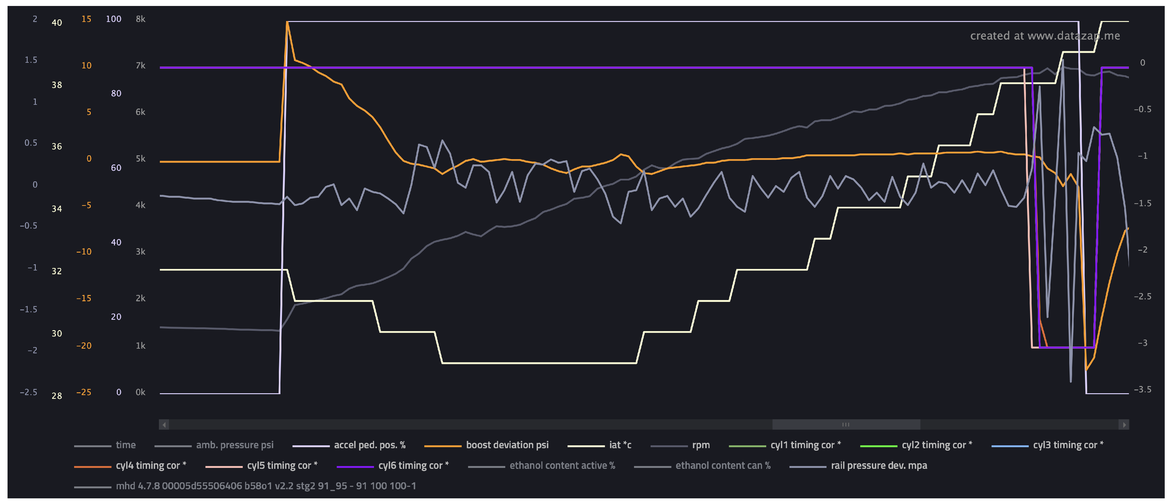
Figure 2.
Uncleaned data log file.
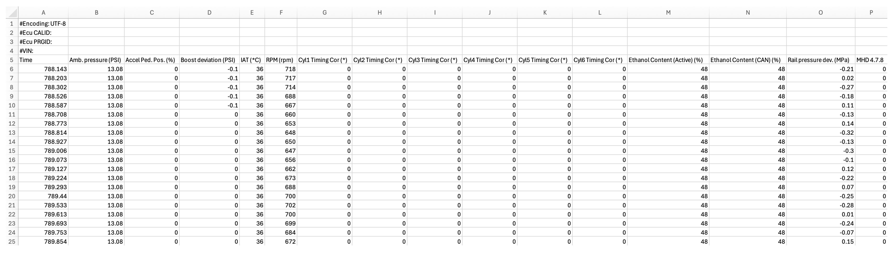
Figure 3.
First few rows of 65.csv.
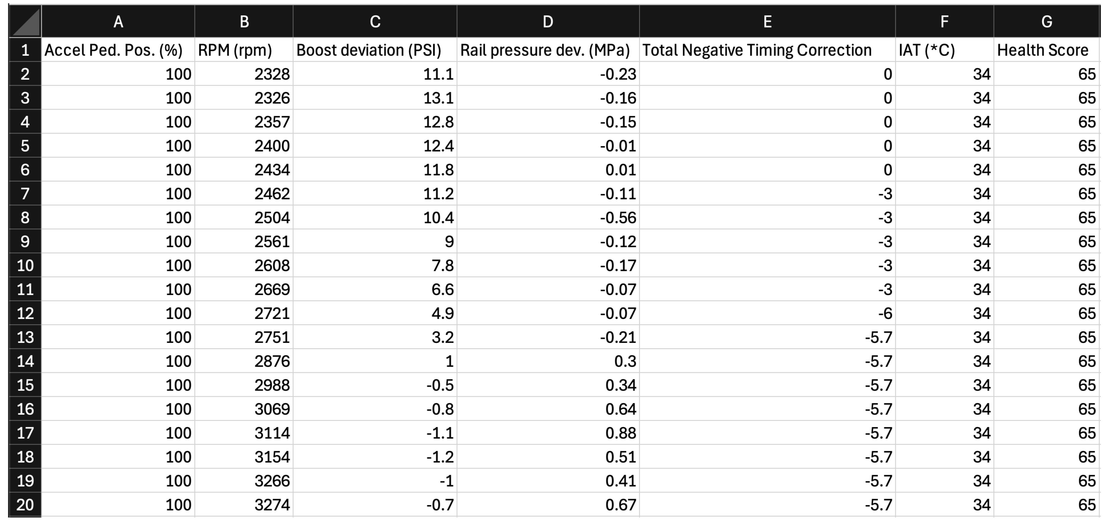
Figure 4.
Training dataset (elevation of 15, azimuth of 45).
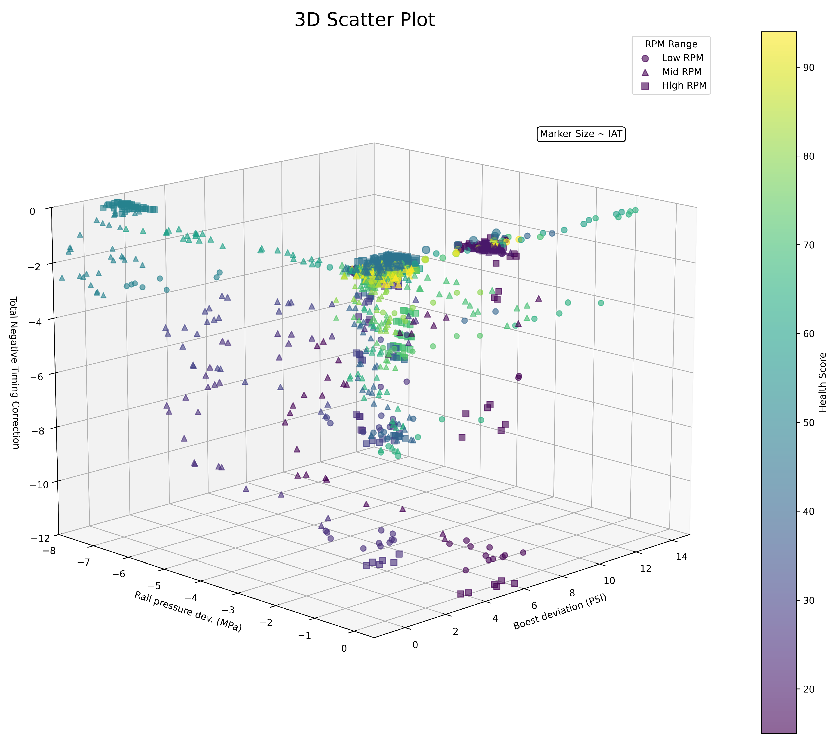
Figure 5.
Pair plot showing trends.
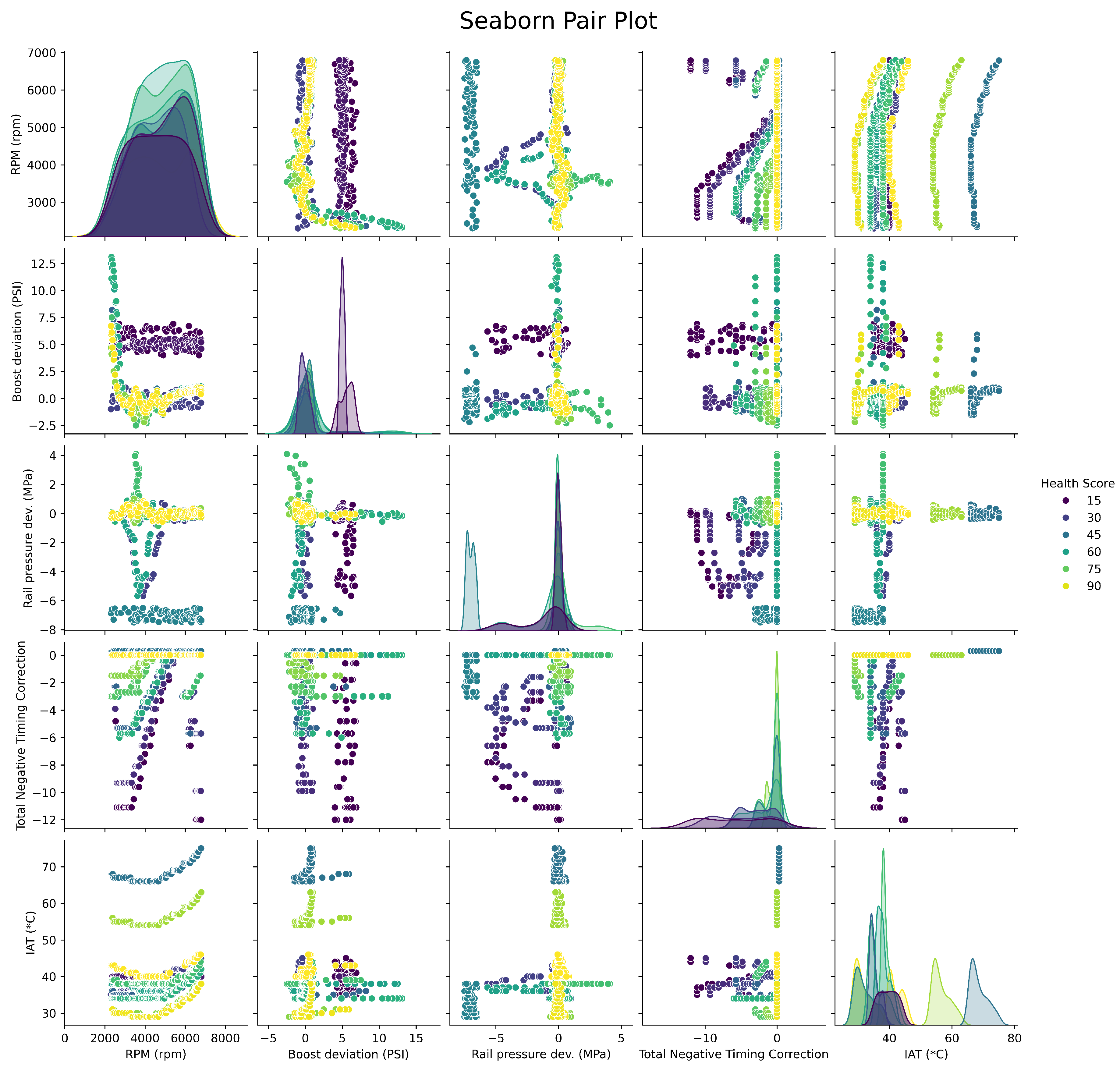
Figure 6.
Heatmap showing correlations.
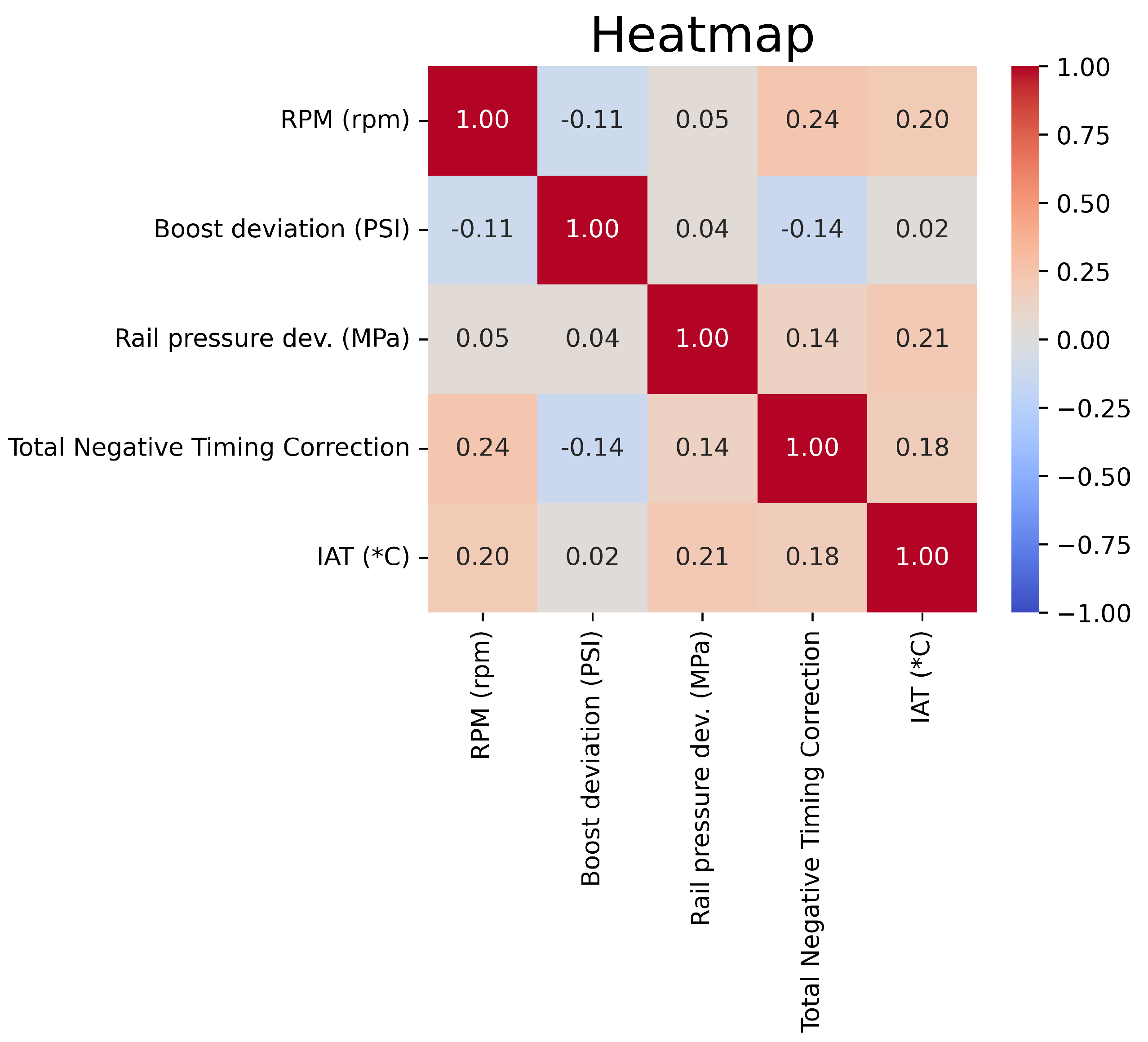
Figure 7.
Principle component analysis showing variance.
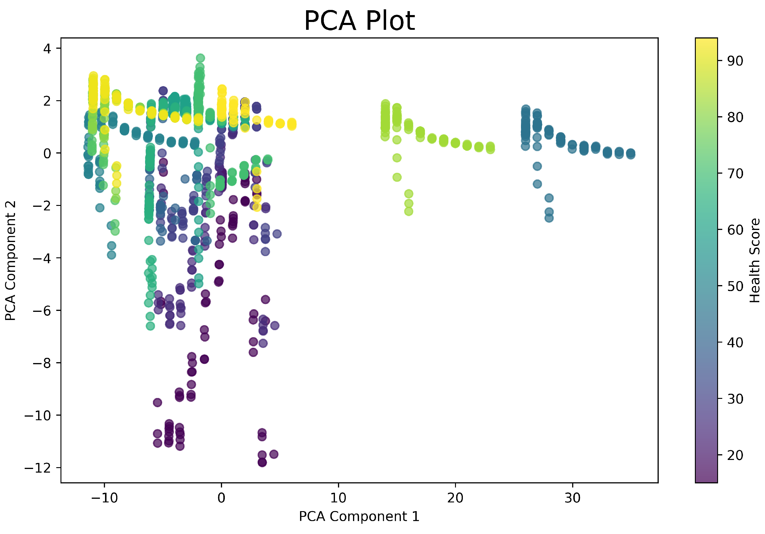
Figure 8.
Parallel coordinates plot showing distribution and variance.
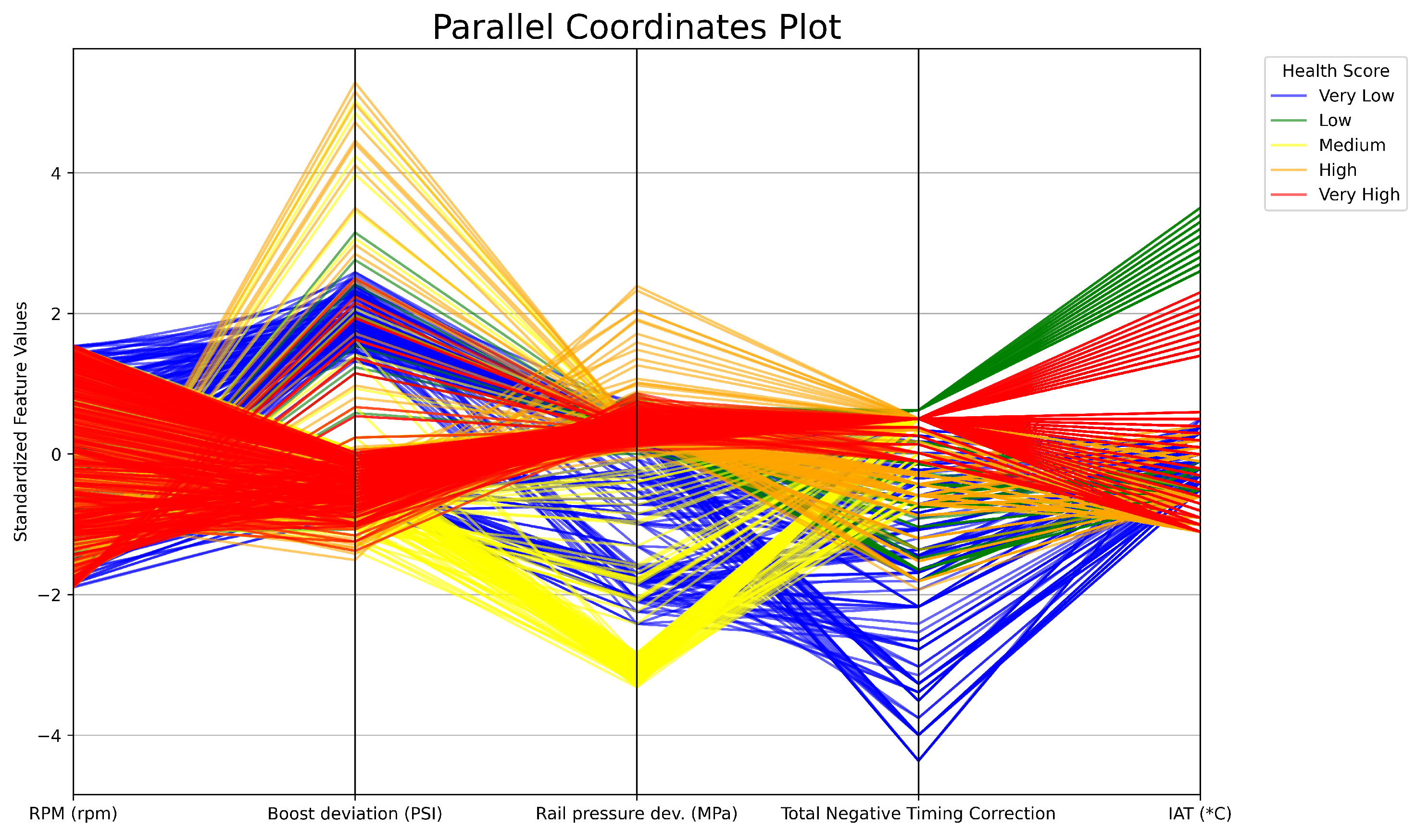
Figure 9.
t-SNE plot showing RPM’s harmonizing effect on the data.
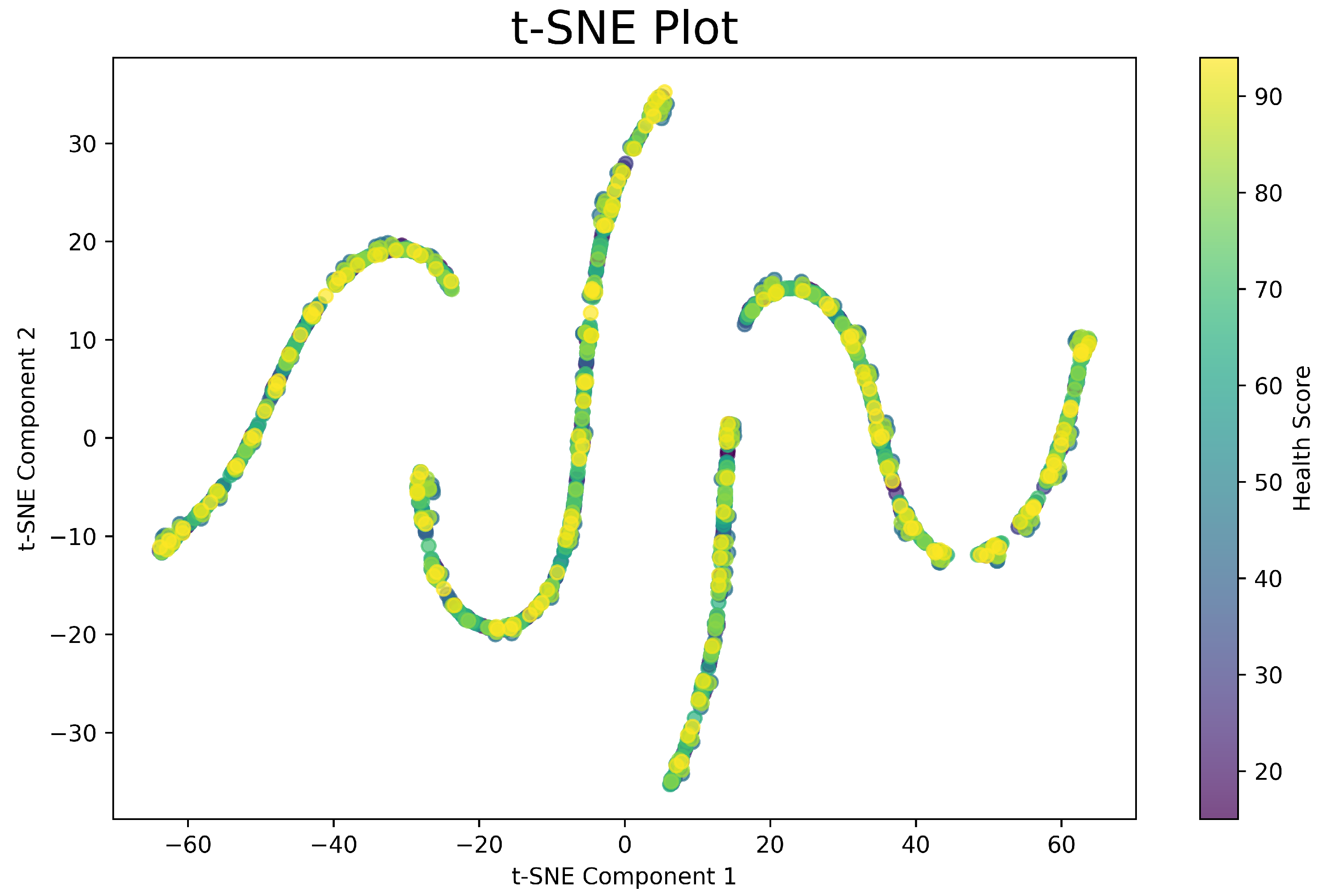
Figure 10.
t-SNE plot showing more disjoint clusters.
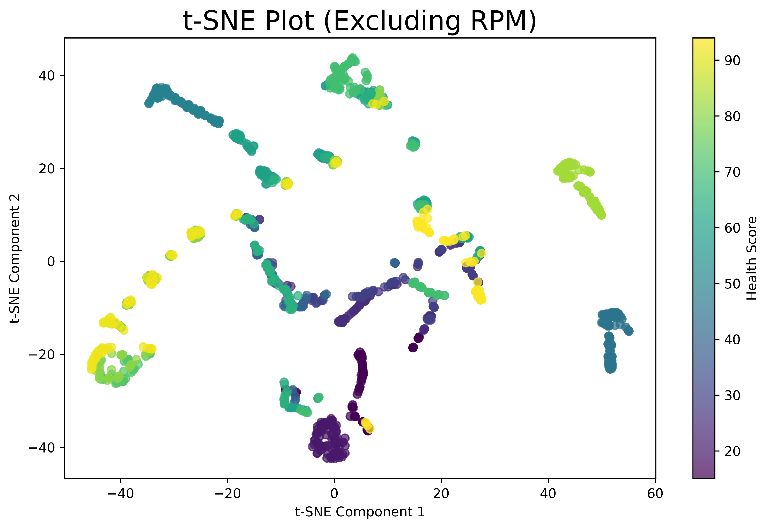

Table 1.
Performance of Models After Tuning Hyperparameters.
| Model | Training Error | Val (30) | Val (65) | Val (90) | Test (45) | Test (70) | ||
|---|---|---|---|---|---|---|---|---|
| KNN | 0.03830 | 30.66 | 64.65 | 90.27 | 45.86 | 70.10 | 1.280 | 0.9647 |
| Extra Trees | 0.1301 | 32.46 | 65.03 | 87.99 | 45.28 | 69.23 | 4.502 | 1.057 |
| XGBoost | 10.88 | 31.85 | 65.41 | 89.86 | 44.63 | 71.26 | 2.402 | 1.639 |
| GBR | 1.414 | 31.07 | 69.71 | 89.96 | 45.15 | 66.32 | 5.812 | 3.824 |
| SVM | 41.19 | 31.66 | 62.69 | 90.01 | 48.26 | 70.89 | 3.985 | 4.157 |
| Random Forest | 28.61 | 30.07 | 69.74 | 89.64 | 43.47 | 65.62 | 5.170 | 5.909 |
| Linear Regression | 354.1 | 52.10 | 65.91 | 64.99 | 57.97 | 64.47 | 48.02 | 18.51 |
14.1cm Figures in the columns Val (30), Val (65), and Val (90) represent the model’s grade on the validation files after tuning. Figures in the columns Test (45) and Test (70) represent the trained model’s grade on the test files.
Disclaimer/Publisher’s Note: The statements, opinions and data contained in all publications are solely those of the individual author(s) and contributor(s) and not of MDPI and/or the editor(s). MDPI and/or the editor(s) disclaim responsibility for any injury to people or property resulting from any ideas, methods, instructions or products referred to in the content. |
© 2024 by the authors. Licensee MDPI, Basel, Switzerland. This article is an open access article distributed under the terms and conditions of the Creative Commons Attribution (CC BY) license (http://creativecommons.org/licenses/by/4.0/).
Copyright: This open access article is published under a Creative Commons CC BY 4.0 license, which permit the free download, distribution, and reuse, provided that the author and preprint are cited in any reuse.


