
Submitted:
16 December 2024
Posted:
17 December 2024
You are already at the latest version
Abstract
The fast-paced depletion of fossil fuels and environmental concerns have intensified interest in renewable energies, with dispatchable solar energy emerging as a key alternative. Concentrated solar power (CSP) technology, utilizing thermal energy storage (TES) systems with molten salts at 560°C, offers significant potential for large-scale energy generation. However, these extreme conditions pose challenges related to material corrosion, critical for maintaining CSP efficiency and lifespan. This research models the corrosion process of 347H stainless steel in molten solar salt (60% NaNO3 + 40% KNO3) melted at 400°C using a cellular automaton (CA) algorithm. The CA model simulates oxide growth under pilot plant conditions in a lattice of 400x400 cells. SEM-EDS imaging compared the model with a mean squared error of 2%, corresponding to a corrosion layer of 4.25 µm after 168 hours. The simulation applied von Neumann and Margolus neighborhoods for ion movement and reaction rules, achieving a cell size of 0.125 µm and 10.08 seconds per iteration. This study demonstrates the CA model’s effectiveness in replicating corrosion processes, offering a tool to optimize material performance in CSP systems.
Keywords:
Cellular automata
; corrosion
; solar energy
; thermal storage
; modeling
; CSP
1. Introduction
Energy transition and the high demand for electricity consumption brings with it a series of challenges and possible problems, especially environmental ones, due to the methods of production used. To meet the growing energy demand and comply with current environmental regulations, new sources of electricity production have been developed, such as solar energy. In recent times, concentrated solar power (CSP) plants have become a promising technology for large-scale electricity production. This technology uses tanks that store thermal energy by employing heat transfer fluid (HTF); this energy is used during the night to produce electricity, thereby maintaining a continuous production cycle [1]. The most used heat transfer medium is a binary mixture of nitrate salts, known as solar salt, composed of 60 % sodium nitrate and 40 % potassium nitrate [1]. Storing thermal energy using molten salts creates extreme operating conditions, reaching over 560 °C, a temperature that affects the materials used in the construction of storage tanks [2,3]. These conditions can cause corrosion damage to the steel used, potentially leading to catastrophic problems for the environment, the plant, or the working personnel [4,5,6,7].
Corrosion study techniques are valuable and provide critical information [8,9,10,11], however, they often require several days or even weeks to complete. To address this, the use of the cellular automata (CA) model is proposed as an alternative for evaluating the corrosion behavior of steel used in thermal storage systems with molten salts [12,13,14]. This approach aims to determine the corrosion rate (C.R.) and simulate oxide formation under the operating conditions of a pilot plant at the University of Antofagasta.
The CA model has been employed by various authors to describe the behavior of natural phenomena, including steel corrosion at different temperatures [15,16,17,18]. Notably, Reinoso-Burrows et al. [19] conducted a comprehensive literature review on the application of this model, focusing on its ability to simulate diverse patterns in the field of corrosion.
The objective of this study is to use the CA model to simulate the formation of corrosion products on 347H stainless steel exposed to molten solar salt at 400 °C. To achieve this, Fe-Cr-Ni elements, representing the main components of the studied steel, were considered. Various corrosion mechanisms for molten nitrate salts have been proposed for these elements. However, most authors have attributed corrosion primarily to nitrate reduction (reaction 1) [7,20,21,22], while dissolved oxygen in the salt has been reported to accelerate corrosion through oxygen reduction (reaction 2) [23].
NO3¯ + 2e¯ ↔ NO2¯ + O2¯
O2 + 4e¯ ↔ 2O2¯
This leads to a series of reactions that govern the corrosion process (reactions 3 to 5). Similarly, the oxide ions present in the molten salt interact not only with iron but also with other key elements in the composition of stainless steel, such as chromium and nickel, as proposed by Mallco et al. [20].
Fe + O2¯ → FeO + 2e¯
3FeO + O2¯ → Fe3O4 + 2e¯
2Fe3O4 + O2¯ → Fe2O3 + 2e¯
2Cr + O2¯ → 3Cr2O3 + 6e¯
2Ni + O2¯ → 2NiO + 2e¯
The present work considers the corrosion mechanism with the above reactions as input data for the model.
2. Methodology: Experimental and Modeling
Immersion Test
The experimental procedure for validating the simulated results involved an immersion test, which included the preparation of stainless steel 347H samples (Table 1). Rectangular samples were cut to dimensions of 300 mm in length, 100 mm in width, and 100 mm in thickness. Each sample was drilled with an 8 mm diameter hole to be placed on the designed rods (Figure 1) for introduction into the pilot molten salt tank (Figure 2).
The samples underwent sanding and polishing treatments up to a 3000-grit size and were weighed in triplicate on an analytical balance ME204T/00 with a precision of ± 0.1 mg before exposure.
After exposure, each sample was removed from the hot tank at 168 h and allowed to cool slowly to room temperature. Excess salt was then removed by rinsing with hot distilled water, acetone, and ethanol, following the ISO/FDIS 17245 standard.
The salt mixture used is solar salt (60% NaNO3 and 40% KNO3) from SQM whose composition is shown in Table 2.
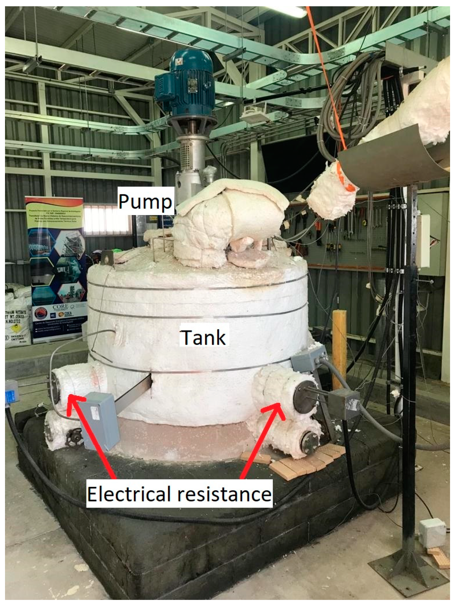
The samples were immersed in 700 kg of solar salt within a the thermal storage tank located in at the University of Antofagasta, Chile. The salt is melted using four 1200-watt electric heaters, reaching an operating temperature of 400°C. The storage system includes a pump that circulates the molten salts within the tank, enabling studies under real operating conditions.
For the SEM/EDS analysis, the cross-sectional corrosion layer of the sample exposed to solar salt needs to be observed. For this purpose, the sample post-exposure was immersed in granular resin heated to 100 °C to be fused with the sample. Subsequently, one side was polished to reveal the steel and the corrosion layer.
Figure 2.
Molten salt thermal storage pilot plant.
Modeling
As part of the methodology, modelling used consists of the following phases: corrosion mechanism, site definition, model parameters and transformation rules.
Corrosion Mechanism
The proposed mechanism considers reactions 3, 4, 5, 6 and 7, which involves a series of reactions of an oxyanion salt. Due to the temperature, the nitrate dissociates, generating the oxide ion (reaction 1). Based on these reactions, various sources of oxide ions are generated. Additionally, this study proposes an extra source corresponding to the reduction of molecular oxygen (reactions 2), which contributes to the concentration of oxide ions in the molten salt mass.
In the long term were only considered hematite, magnetite, chromium oxide and nickel oxide elements in the model from the proposed mechanism, because the model does not consider intermediate reactions and in the long term the presence of FeO at high temperatures is not reported. Because of this, the reactions considered were the following:
3Fe + 4O2¯ → Fe3O4
2Fe3O4 + O2¯ → 3Fe2O3
2Cr + 3O2¯ → Cr2O3
Ni + O2¯ → NiO
Site Definition
A 2-dimensional cellular automaton model was developed within a 400x400 cell grid. To define the sites and facilitate the calculation process, letters representing the compounds and elements involved in the corrosion process were assigned to each cell of the grid, as shown in the Figure 3, with the corresponding letters displayed in the Table 3. All elements are considered fixed, except for site B, which is mobile and can move throughout the entire grid. The initial concentrations of sites A, E, and G (representing elements of Fe, Cr, and Ni, respectively) were 73.5%, 17.5% and 9% respectively. The oxide ion is represented by site B and the corrosion sites C, D, F and H, corresponding to Fe3O4, Fe2O3, Cr2O3, and NiO respectively, were generated throughout the simulation.
The proposed corrosion mechanism, combined with the labeling of elements and compounds involved in the simulation, serves as the foundation for the model's simplified equations. This approach is designed to optimize computation time and streamline the analysis of the model's results.
A + B → C
C + B → D
E + B → F
G + B → H
Model Parameters
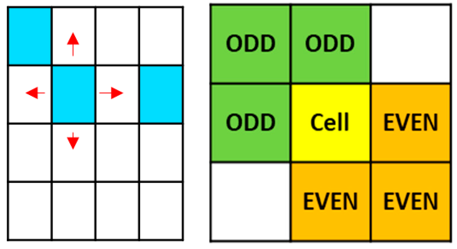
Site B was considered the main corrosive agent in the model. Its movement utilized the von Neumann neighborhood and could move randomly across the entire grid and the reaction rules used the Margolus neighborhood, to reduce programming times.
Figure 4.
(a) Von Neumann and (b) Margolus neighborhood.
Movement probabilities were assigned to site B only when it was adjacent to any site F, corresponding to chromium oxide representing chromium passivation elements seen in the Figure 5. The probabilities were: Pd4 < Pd3 < Pd2 < Pd1 < Pd0, corresponding to 0.2, 0.4, 0.6, 0.8, and 1.0 respectively. Additionally, a constant concentration of 25% was considered in each iteration.
Transformation Rules
Once site B completed its movement, the Margolus neighborhood was applied to determine the reaction and transformation rules. Seventeen possible cases were defined according to each site on the grid. The Figure 6 shows the five possible cases for site A, each possibility having a probability of occurrence based on the relative probability of oxidation, which considers the standard reduction potential using the equation 16 whose results are shown in the Table 4.
3. Results
SEM/EDS
The SEM cross sections results are shown in the Figure 7. The sample exposed to 400 °C for 168 hours in solar salt was used.
The EDS mapping is shown in the Figure 8, which displays the concentration of Cr as an important element in the corrosion resistance of stainless steel 347H. Black areas indicate zones with low or no chromium concentration, while fluorescent green highlights areas with the presence of chromium. From left to right in the image, a transition can be observed from low or no chromium concentration to an increase in chromium concentration within the steel, as shown on the right side of the image.
Modeling
Initially, 100,000 iterations were simulated. Figure 9 shows the general behavior of evolution in the concentration of all the sites in the model. As the simulation progresses, the concentration of the metallic sites A (Fe), E (Cr), and G (Ni) decreases, and due to the reaction and transformation rules, they are converted into corrosion products C, D, F, and H, which increase their concentration over time showed in Figure 10.
Figure 11 shows the concentrations of simulated sites at 60.000 iterations with respect to the metal depth, which corresponds to 200 cells. The X-axis represents the steel depth in terms of cell count, while the Y-axis indicates the sum of sites for the different simulated elements. Initially, there is a lower concentration of sites A, E, and G, up to approximately 34 cells, which marks the end of the corrosion layer. Furthermore, in areas with reduced concentrations of Fe, Cr, and Ni due to the corrosion process, the model generates sites C, D, F, and H, which correspond to the simulated corrosion products.
Figure 12 shows the cross-section of the model, and the evolution of the corrosion layer throughout the simulation.
Data Processing
Data processing was made to simulate results with respect to the experimental EDS results shown in Figure 13. The mean squared error between the simulated curve and the EDS data was calculated, resulting in a 2% error at 60.000 steps, the lowest among all simulation times. This corresponds to 168 hours of exposure, with each iteration representing 10.08 seconds and a cell size of 0.125 µm.
4. Conclusions
The results obtained through SEM/EDS allowed the identification of areas with a lower concentration of key elements involved in the corrosion process, which was fundamental for providing experimental validation of the simulated results. These results indicate that each iteration corresponds to 10.08 experimental seconds, and each cell in the mesh represents 0.125 µm, with a corrosion layer thickness of 4.25 µm in the studied steel. The model achieved an error of 2% at 60.000 iterations. Although the model was refined to achieve a low error rate, further validation and adjustments could potentially reduce it even further.
This study represents progress in simulating the corrosion process in thermal storage systems with molten salts. The results indicate that the cellular automaton model can replicate the formation of expected corrosion products under the operating conditions of a pilot plant. However, a significant gap remains to be addressed regarding the use of the CA model. One challenge is simulating more complex corrosion mechanisms, and another is obtaining a greater amount of experimental data at the scale of a pilot plant.
Concerning transfer of knowledge, data investigated in this study was used as content used in a virtual reality concept, that shall facilitate the transmission of knowledge as well as to enhance the dissemination of results.
Author Contributions
Conceptualization, J.C.R-B. and M.C-C.; methodology, J.C.R-B, M.C-C., M.H.; software, J.C.R-B, C.S., A.A,; validation, J.C.R-B, M.C-C. and M.H., formal analysis, J.C.R-B., F.G-M.,; investigation, J.C.R-B., M.H.; resources, L.G..; data curation, J.C.R-B.; writing—original draft preparation, J.C.R-B.; writing—review and editing, J.C.R-B., M.H., C.S., C.D, E.F., L.G, F.G-M., R.P,; visualization, J.C.R-B.; supervision, J.C.R-B., M.C-C., E.F., F.G-M.; project administration, J.C.R-B. All authors have read and agreed to the published version of the manuscript.
Funding
The authors gratefully acknowledge the financial support of the Project VR4Learning (Project nr. 2022-2-SE02-KA220-YOU-000100999) for in-valuable support with SEM and publication. Funded by the European Union.
Institutional Review Board Statement
Not applicable.
Informed Consent Statement
Not applicable.
Data Availability Statement
The original contributions presented in the study are included in the
article, further inquiries can be directed to the corresponding author.
Acknowledgments
The authors are grateful for the support of ANID-Chile through the research projects, ANID code VIU24P0174, CONICYT/FONDAP 1523A0006 “Solar Energy Research Center” SERC-Chile, Engineering Project 2030 Code 16ENl2-71940 of Corfo, Government of Chile, and Grateful to Doctoral Program in Solar Energy Universidad de Antofagasta, Chile
Conflicts of Interest
The authors declare no conflicts of interest.
References
- Palacios, A. ; C. Barreneche, M. E. Navarro, and Y. Ding, “Thermal energy storage technologies for concentrated solar power – A review from a materials perspective,” Aug. 01, 2020, Elsevier Ltd. [CrossRef]
- M. Walczak, F. Pineda, Á. G. Fernández, C. Mata-Torres, and R. A. Escobar, “Materials corrosion for thermal energy storage systems in concentrated solar power plants,” Apr. 01, 2018, Elsevier Ltd. [CrossRef]
- F. Vilchez, F. Pineda, M. Walczak, and J. Ramos-Grez, “The effect of laser surface melting of stainless steel grade AISI 316L welded joint on its corrosion performance in molten Solar Salt,” Solar Energy Materials and Solar Cells, vol. 213, Aug. 2020. [CrossRef]
- J. D. Osorio et al., “Failure Analysis for Molten Salt Thermal Energy Storage Tanks for In-Service CSP Plants,” 2024. [Online]. Available: www.nrel.gov/publications.
- B. Lucas Granados, B. Lucas Granados, and R. Sanchez Tovar, Corrosion. Editorial de la Universidad Politecnica de Valencia, 2018. [Online]. Available: https://elibro.net/es/lc/uantof/titulos/57467.
- M. Sarvghad, T. A. Steinberg, and G. Will, “Corrosion of stainless steel 316 in eutectic molten salts for thermal energy storage,” Solar Energy, vol. 172, pp. 198–203, Sep. 2018. [CrossRef]
- S. Bell, T. Steinberg, and G. Will, “Corrosion mechanisms in molten salt thermal energy storage for concentrating solar power,” Oct. 01, 2019, Elsevier Ltd. [CrossRef]
- C.Prieto et al., “Study of corrosion by Dynamic Gravimetric Analysis (DGA) methodology. Influence of chloride content in solar salt,” Solar Energy Materials and Solar Cells, vol. 157, pp. 526–532, Dec. 2016. [CrossRef]
- A.G. Fernández, A. Rey, I. Lasanta, S. Mato, M. P. Brady, and F. J. Pérez, “Corrosion of alumina-forming austenitic steel in molten nitrate salts by gravimetric analysis and impedance spectroscopy,” Materials and Corrosion, vol. 65, no. 3, pp. 267–275, Mar. 2014. [CrossRef]
- V. Encinas-Sánchez, M. T. de Miguel, M. I. Lasanta, G. García-Martín, and F. J. Pérez, “Electrochemical impedance spectroscopy (EIS): An efficient technique for monitoring corrosion processes in molten salt environments in CSP applications,” Solar Energy Materials and Solar Cells, vol. 191, pp. 157–163, Mar. 2019. [CrossRef]
- N. Juan Mendoza Flores, R. Durán Romero, J. Genescá Llongueras, and I. Electroquímica JMF, “ESPECTROSCOPÍA DE IMPEDANCIA ELECTROQUÍMICA EN CORROSIÓN.
- W. Wang, B. Guan, X. Wei, J. Lu, and J. Ding, “Cellular automata simulation on the corrosion behavior of Ni-base alloy in chloride molten salt,” Solar Energy Materials and Solar Cells, vol. 203, Dec. 2019. [CrossRef]
- Z. Xu, X. Wei, J. Lu, J. Ding, and W. Wang, “Simulation of corrosion behavior of Fe–Cr–Ni alloy in binary NaCl–CaCl2 molten salt using a cellular automata method,” Solar Energy Materials and Solar Cells, vol. 231, Oct. 2021. [CrossRef]
- Z. Xu, J. Lu, X. Wei, J. Ding, and W. Wang, “2D and 3D cellular automata simulation on the corrosion behaviour of Ni-based alloy in ternary molten salt of NaCl–KCl–ZnCl2,” Solar Energy Materials and Solar Cells, vol. 240, Jun. 2022. [CrossRef]
- J. Stafiej, D. Di Caprio, and Ł. Bartosik, “Corrosion-passivation processes in a cellular automata based simulation study,” Journal of Supercomputing, vol. 65, no. 2, pp. 697–709, Aug. 2013. [CrossRef]
- S. Guiso, D. di Caprio, J. de Lamare, and B. Gwinner, “Intergranular corrosion: Comparison between experiments and cellular automata,” Corros Sci, vol. 177, Dec. 2020. [CrossRef]
- C. F. Pérez-Brokate, D. di Caprio, D. Féron, J. de Lamare, and A. Chaussé, “Probabilistic cellular automata model of generalised corrosion, transition to localised corrosion,” Corrosion Engineering Science and Technology, vol. 52, pp. 186–193, Apr. 2017. [CrossRef]
- H. Chen, Y. Chen, and J. Zhang, “Cellular automaton modeling on the corrosion/oxidation mechanism of steel in liquid metal environment,” Progress in Nuclear Energy, vol. 50, no. 2–6, pp. 587–593, Mar. 2008. [CrossRef]
- J. C. Reinoso-Burrows, N. Toro, M. Cortés-Carmona, F. Pineda, M. Henriquez, and F. M. Galleguillos Madrid, “Cellular Automata Modeling as a Tool in Corrosion Management,” Sep. 01, 2023, Multidisciplinary Digital Publishing Institute (MDPI). [CrossRef]
- A. Mallco, C. Portillo, M. J. Kogan, F. Galleguillos, and A. G. Fernández, “A materials screening test of corrosion monitoring in LiNO3 containing molten salts as a thermal energy storage material for CSP plants,” Applied Sciences (Switzerland), vol. 10, no. 9, May 2020. [CrossRef]
- A.S. Dorcheh, R. N. Durham, and M. C. Galetz, “High temperature corrosion in molten solar salt: The role of chloride impurities,” Materials and Corrosion, vol. 68, no. 9, pp. 943–951, Sep. 2017. [CrossRef]
- Á.G. Fernández and L. F. Cabeza, “Molten salt corrosion mechanisms of nitrate based thermal energy storage materials for concentrated solar power plants: A review,” Solar Energy Materials and Solar Cells, vol. 194, pp. 160–165, Jun. 2019. [CrossRef]
- J. M. De Jong and G. H. J. Broers, “A REVERSIBLE OXYGEN ELECTRODE IN AN EQUIMOLAR KNO,-NaNO, MELT SATURATED WITH SODIUM PEROXIDE-II. A VOLTAMMETRIC STUDY.
Figure 1.
Coupon holder designed for pilot plant.

Figure 3.
Distribution of sites in cellular automata matrix.
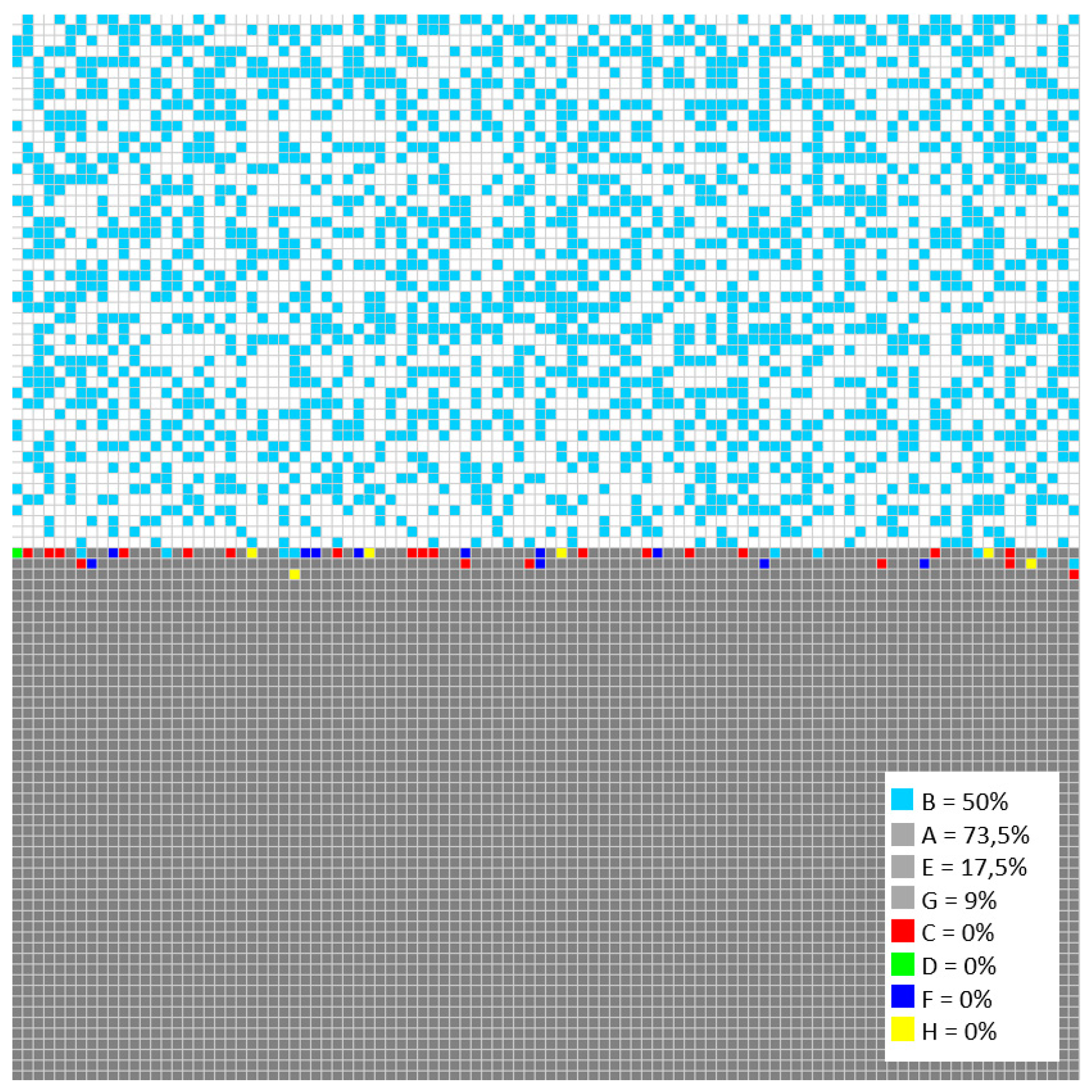
Figure 5.
Probability of motion for site B.
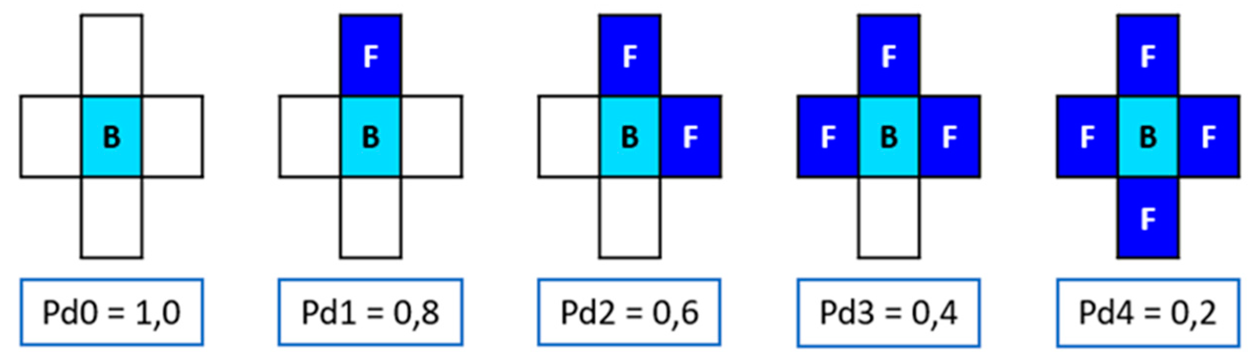
Figure 6.
Reaction and transformation rules for site A.
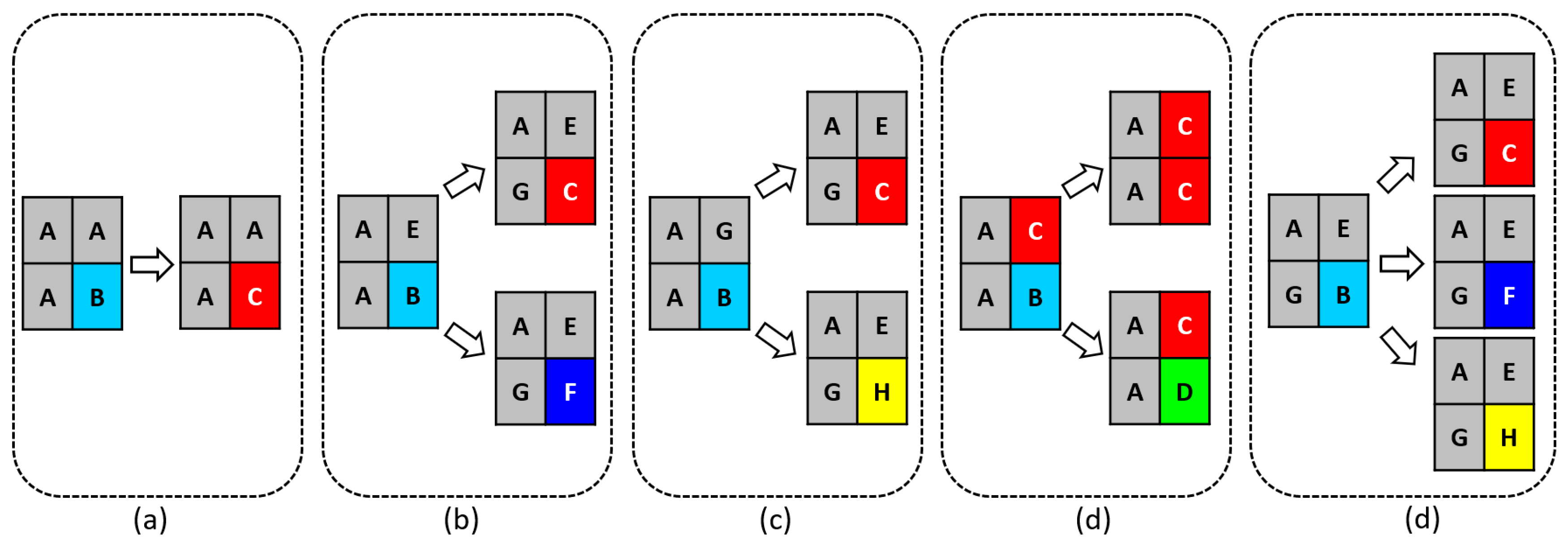
Figure 7.
SEM cross-section of sample 168h.
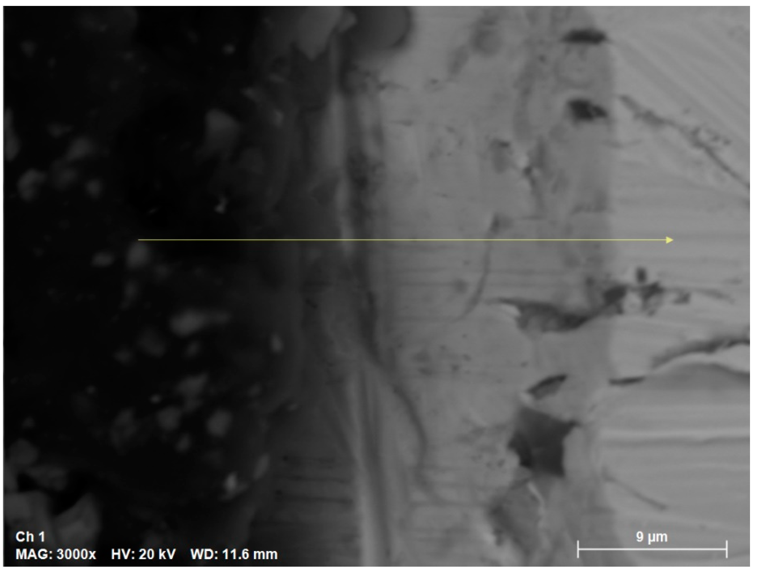
Figure 8.
Mapping EDS cross section of sample 168h.
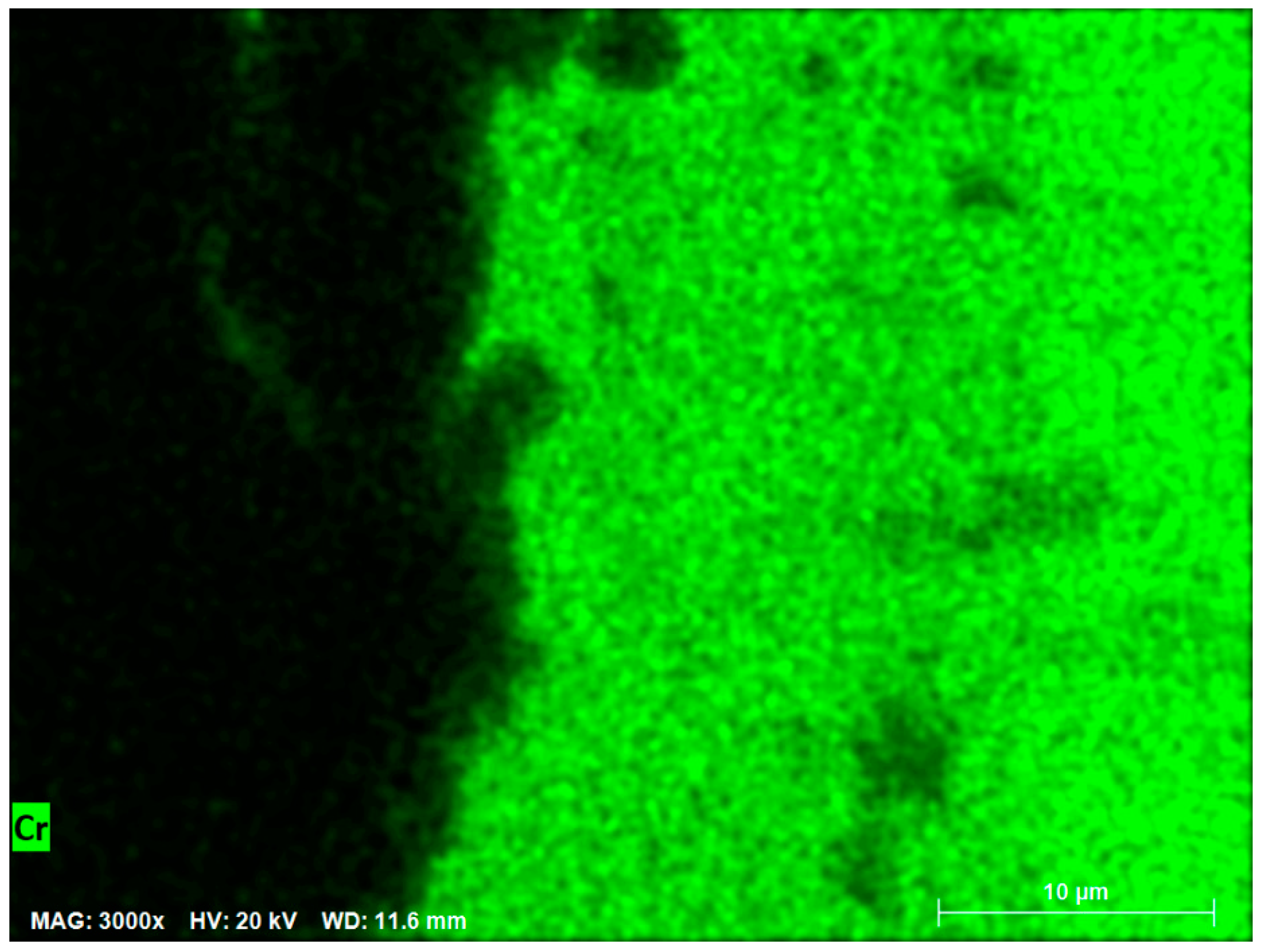
Figure 9.
Concentration of sites A, E, and G after 100,000 iterations with 25% B sites.
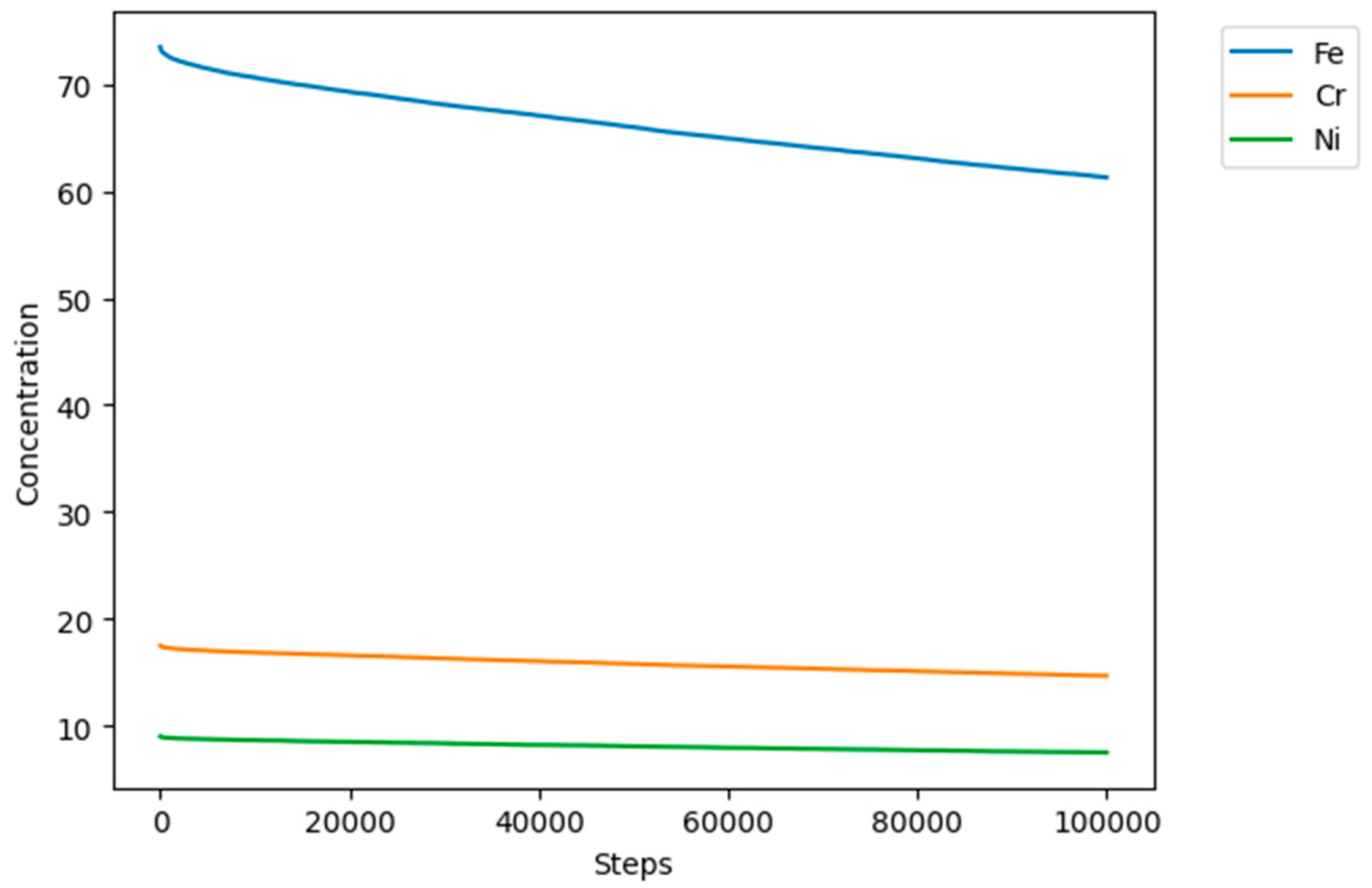
Figure 10.
Concentration of sites C, D, F and H after 100,000 iterations with 25% B sites.
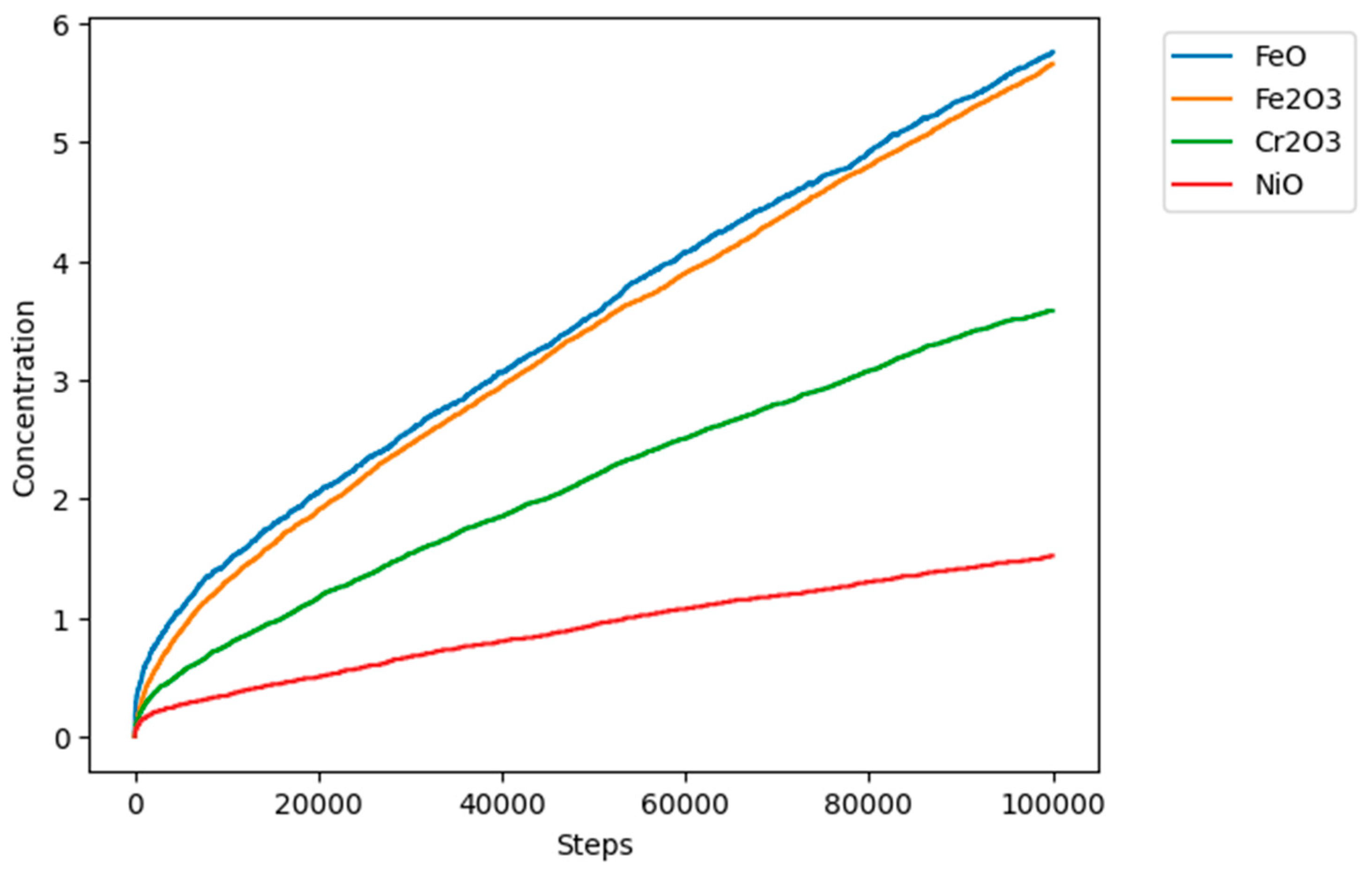
Figure 11.
Evolution of the concentration of simulated elements at 60.000 iterations.
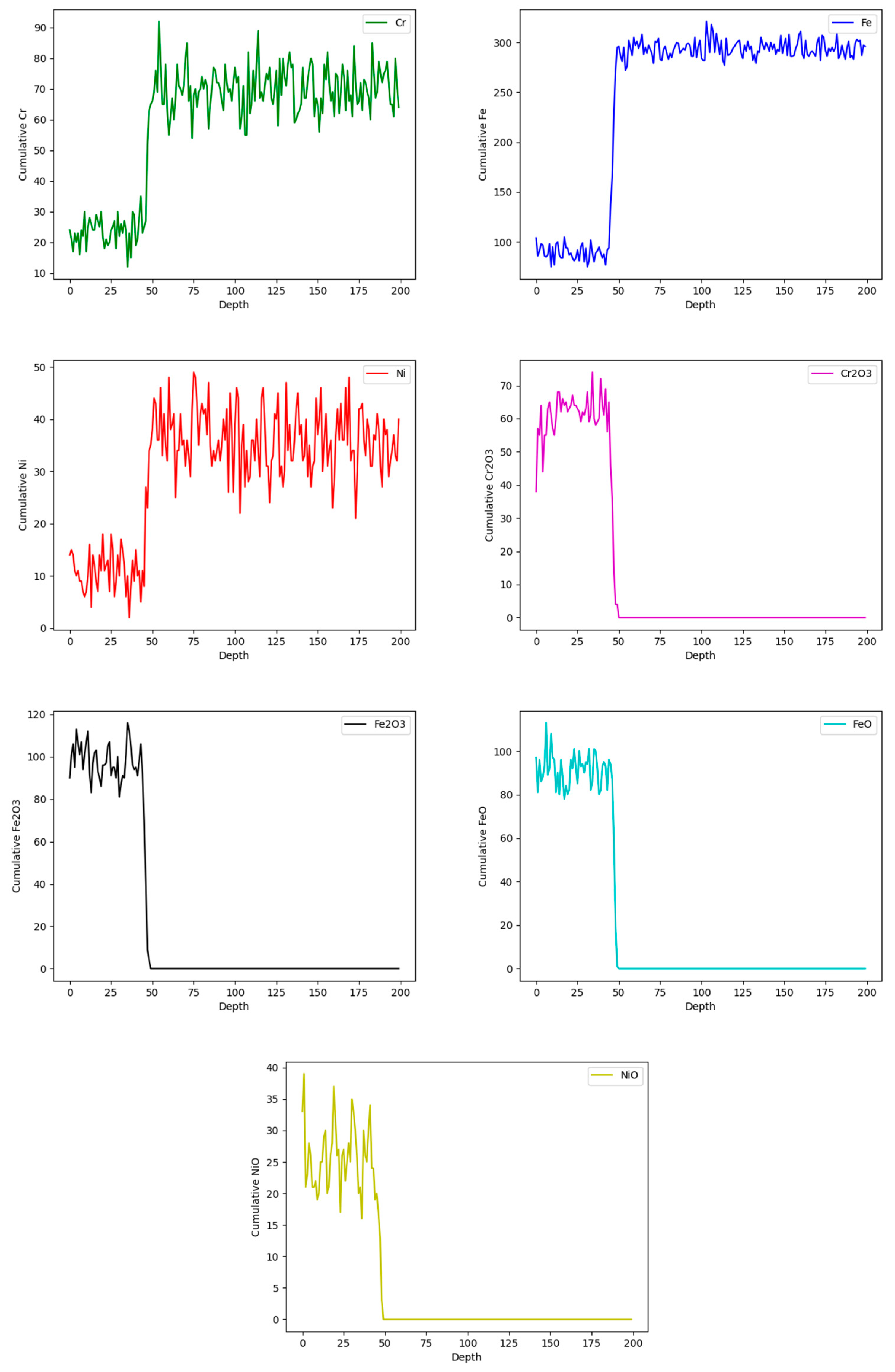
Figure 12.
Cross-sectional view of the corrosion layer growth at 1.000, 20.000, 40.000, and 60.000 steps.
Figure 12.
Cross-sectional view of the corrosion layer growth at 1.000, 20.000, 40.000, and 60.000 steps.

Figure 13.
Comparison of EDS curve for the 168h sample versus chromium site concentration at 60.000 steps.
Figure 13.
Comparison of EDS curve for the 168h sample versus chromium site concentration at 60.000 steps.
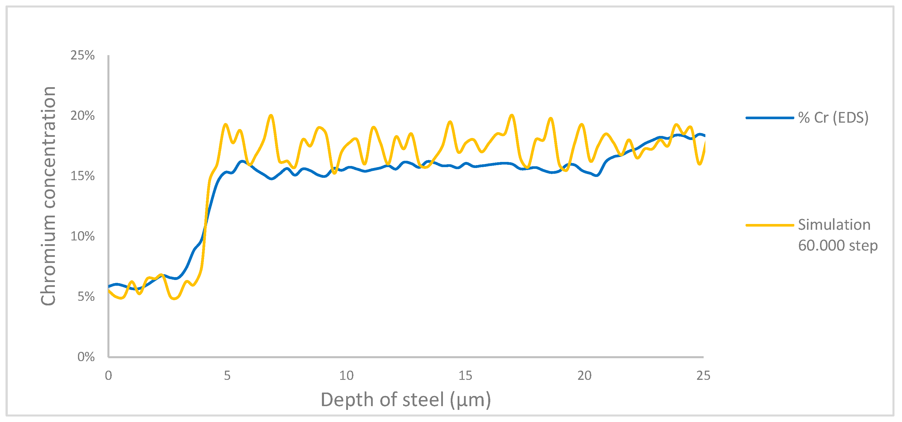

Table 1.
Chemical composition SS 347H.
| Chemical composition of stainless steel AISI 347H [%p/p] | |||||||||||
| Fe | C | Si | Mn | Cr | Mo | Ni | Al | Co | Cu | Nb | W |
| 70.5 | 0.04565 | 0.1885 | 1.735 | 17.05 | 0.396 | 8.96 | 0.0068 | 0.114 | 0.4195 | 0.4015 | 0.0378 |
Table 2.
Chemical composition of solar salt.
| Solar salt – chemical composition | |
| Compound | [%p/p] |
| NaNO3 | 60.2 |
| KNO3 | 39.8 |
Table 3.
Labeling of elements and compounds involved in the simulation.
| Fe | O2- | Fe3O4 | Fe2O3 | Cr | Cr2O3 | Ni | NiO |
| A | B | C | D | E | F | G | H |
Table 4.
Relative probability according to standard reduction potential.
| Site | Element | E° (V) | P.ox_rel | P.rel₁ (%) | P.rel₂ (%) | P.rel₃ (%) | P.rel₄ (%) |
| A | Fe | -0.44 | 1.55 | 31.4 | 57.4 | - | 54.6 |
| E | Cr | -0.74 | 2.09 | 42.4 | 42.6 | 61.8 | - |
| G | Ni | -0.25 | 1.29 | 26.2 | - | 38.2 | 45.4 |
Disclaimer/Publisher’s Note: The statements, opinions and data contained in all publications are solely those of the individual author(s) and contributor(s) and not of MDPI and/or the editor(s). MDPI and/or the editor(s) disclaim responsibility for any injury to people or property resulting from any ideas, methods, instructions or products referred to in the content. |
© 2024 by the authors. Licensee MDPI, Basel, Switzerland. This article is an open access article distributed under the terms and conditions of the Creative Commons Attribution (CC BY) license (http://creativecommons.org/licenses/by/4.0/).
Copyright: This open access article is published under a Creative Commons CC BY 4.0 license, which permit the free download, distribution, and reuse, provided that the author and preprint are cited in any reuse.


