4. Experimental Analysis
The precision of the terrain data in this experiment is 12.5 meters. Using the calculation formula of the neighborhood range, the Eps range for the experiment should fall within [
13,
20].
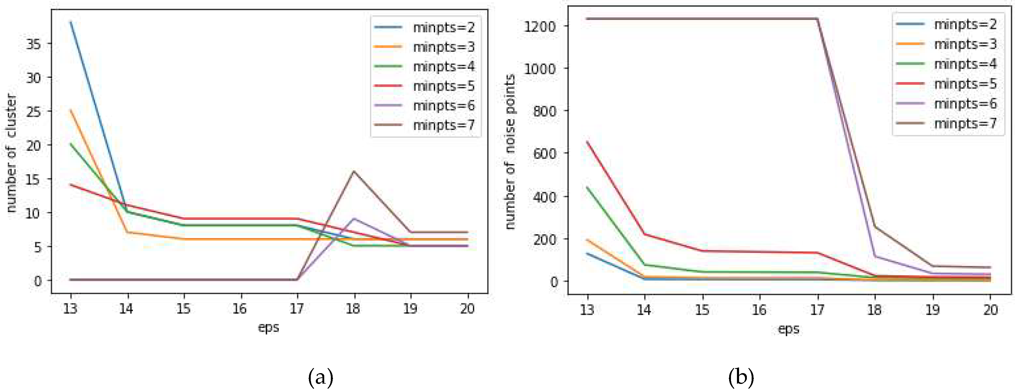
Figure 3 illustrates the fluctuation in the number of clusters and noise data as the neighborhood radius varies when MinPts lies between 2 and 7.
Figure 3 illustrates the outcomes of the cluster analysis.
Figure 3(a) and
Figure 3(b) depict the number of clusters and noise points derived from clustering under varying parameters such as neighborhood radius Eps and minimum sample points MinPts. As indicated in
Figure 3, there is a fluctuation in the number of clusters under different minimum sample points. When MinPts is 6 and 7, and Eps is 17 or 18, the number of clusters and noise points shows significant changes but remains unchanged as parameters increase further. Consequently, this parameter is not beneficial for parameter selection and should be excluded. Similarly, when MinPts equals 2 or 3, the number of clusters also experiences a sudden change before stabilizing. In that case, there are fewer noise points, but the number of clusters suddenly decreases with changes in the neighborhood radius. This is attributed to isolated noise points whose quantity exceeds two, and these two or more points are proximate. They are classified into a cluster under a lower neighborhood radius Eps. As the neighborhood radius increases, the genuine clusters merge the classes composed of noise data. This situation can misguide the choice of Eps results; hence, it needs to be excluded. When MinPts equals 4 or 5, neither of these situations occurs that will cause a significant change in the number of clusters. However, when MinPts equals 5, the volume of noise data surpasses that when MinPts equals 4, as shown in
Figure 3(b). Given that this study focuses on the viewshed and aims to incorporate more visible points in subsequent analysis, it is currently necessary to have relatively fewer noise data and include more visible points in the viewshed analysis. Therefore, choosing MinPts as 4 is more rational, and with this parameter value, the number of clusters changes less as Eps changes, so one can more precisely choose the neighborhood radius value. When selecting the value of Eps, it should ensure that both the number of noise data and clusters are relatively low and they do not change with the increase in neighborhood radius. As shown in
Figure 3(a), when Eps is 18, it can meet conditions such as fewer clusters, no further changes with increasing neighborhood radius, and relatively fewer noise data. Therefore, choosing 18 meters as the neighborhood radius is appropriate.
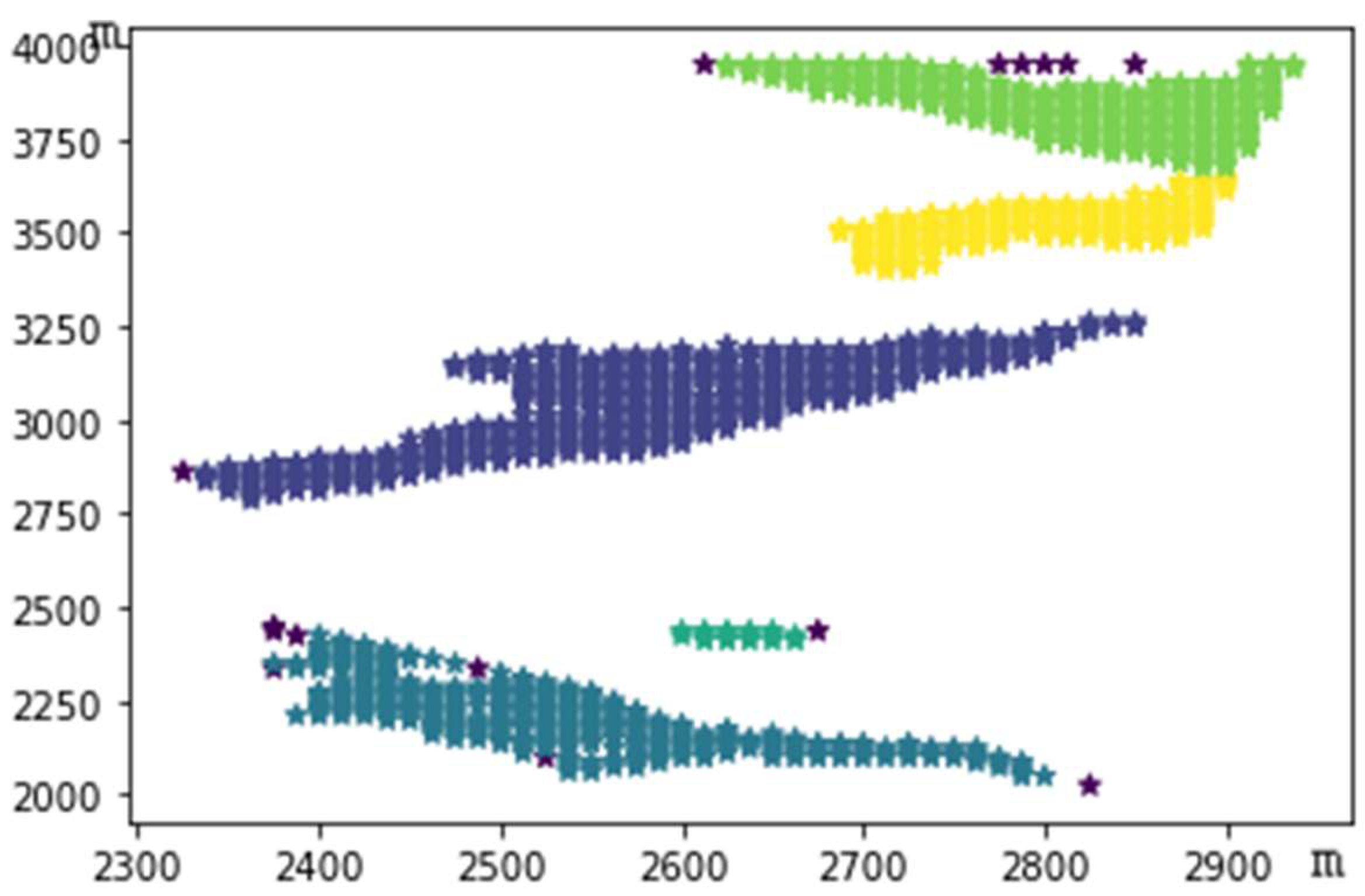
Consequently, clustering was executed with a minimum sample point count of 4 and a neighborhood radius of 18 meters, yielding the results depicted in
Figure 4.
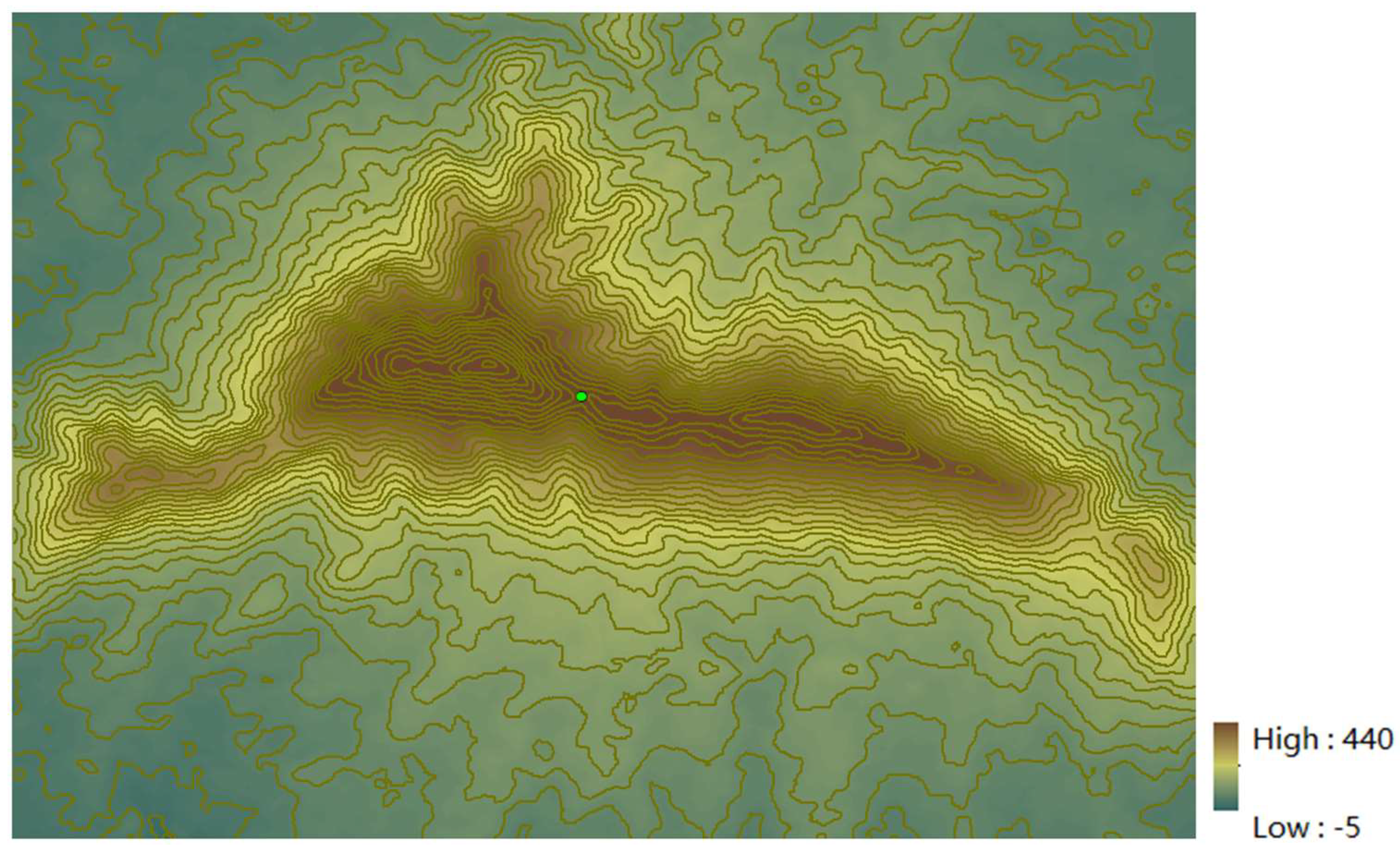
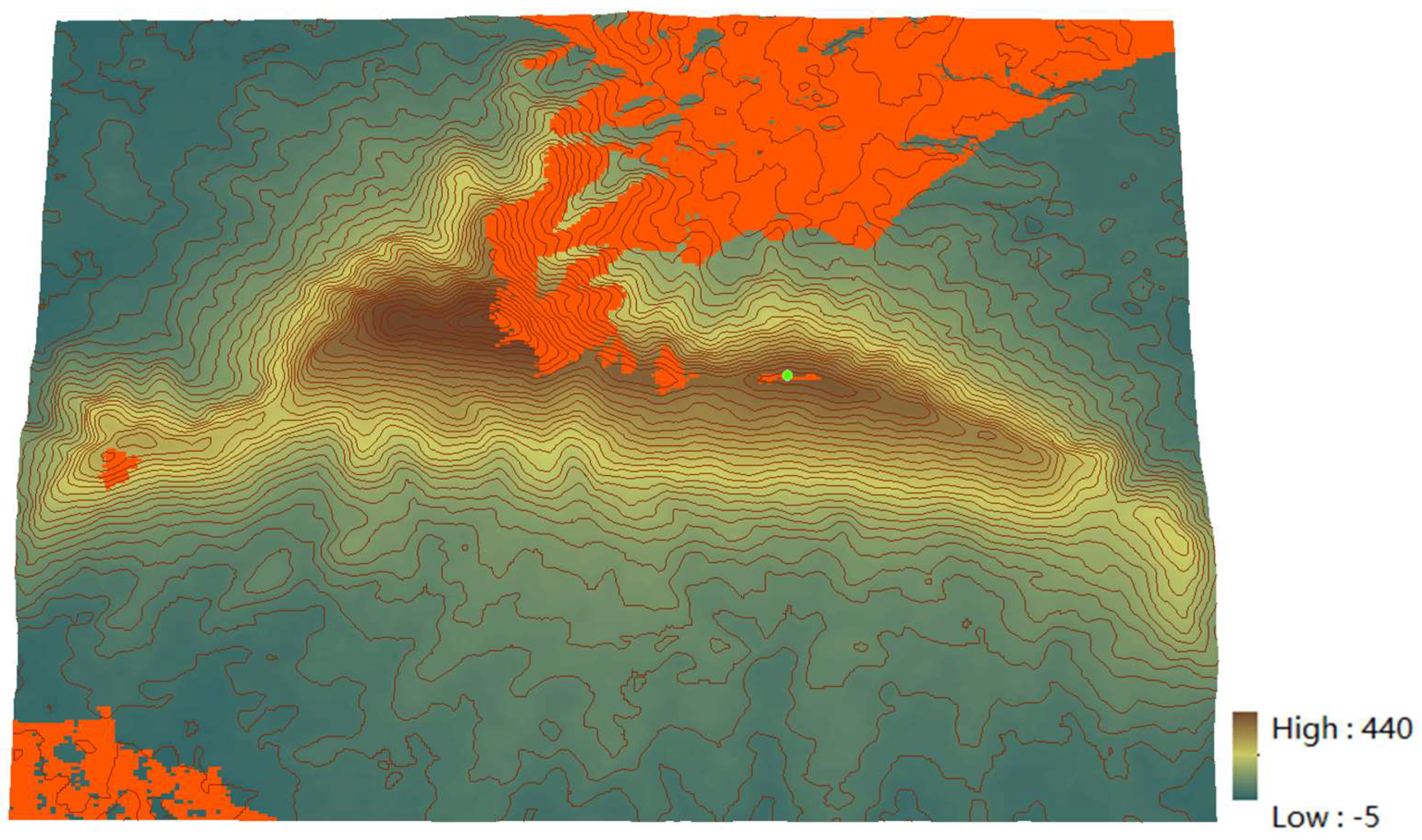
The observation point is located at [2725, 2112.5, 334], with the longitude and latitude (118.845°E, 32.071°N) situated at a higher position on Purple Mountain, as shown in
Figure 1. A DBSCAN clustering analysis was conducted on the viewshed of the observation point, and the division after clustering is shown in
Figure 4. The entire viewshed is divided into five sub-viewsheds with 13 noise points.
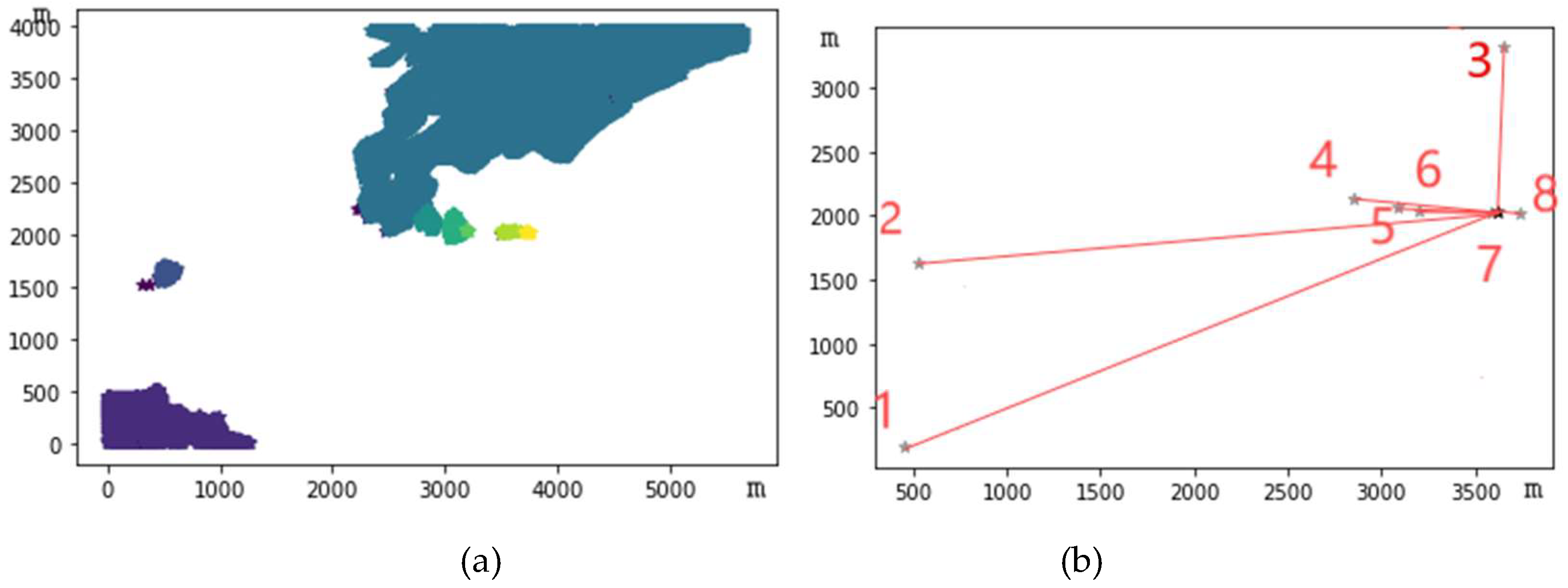
Figure 4 displays the results of the division, where the coordinate axis uses the southwest edge of the map as the origin, with 12.5 meters as one grid precision, and relative coordinates represent the distance relationship between each sub-viewshed.
The overall distribution of the visible points is relatively uniform, with its essential distribution characteristics being that two sub-viewsheds are far apart or not adjacent. For points that are distributed adjacently and clustered together, it can be considered that the distance between the two points is less than or equal to the neighborhood radius value of 18 meters, and the number of sample points within the neighborhood range centered on a specific point reaches the minimum sample point number value of 4.
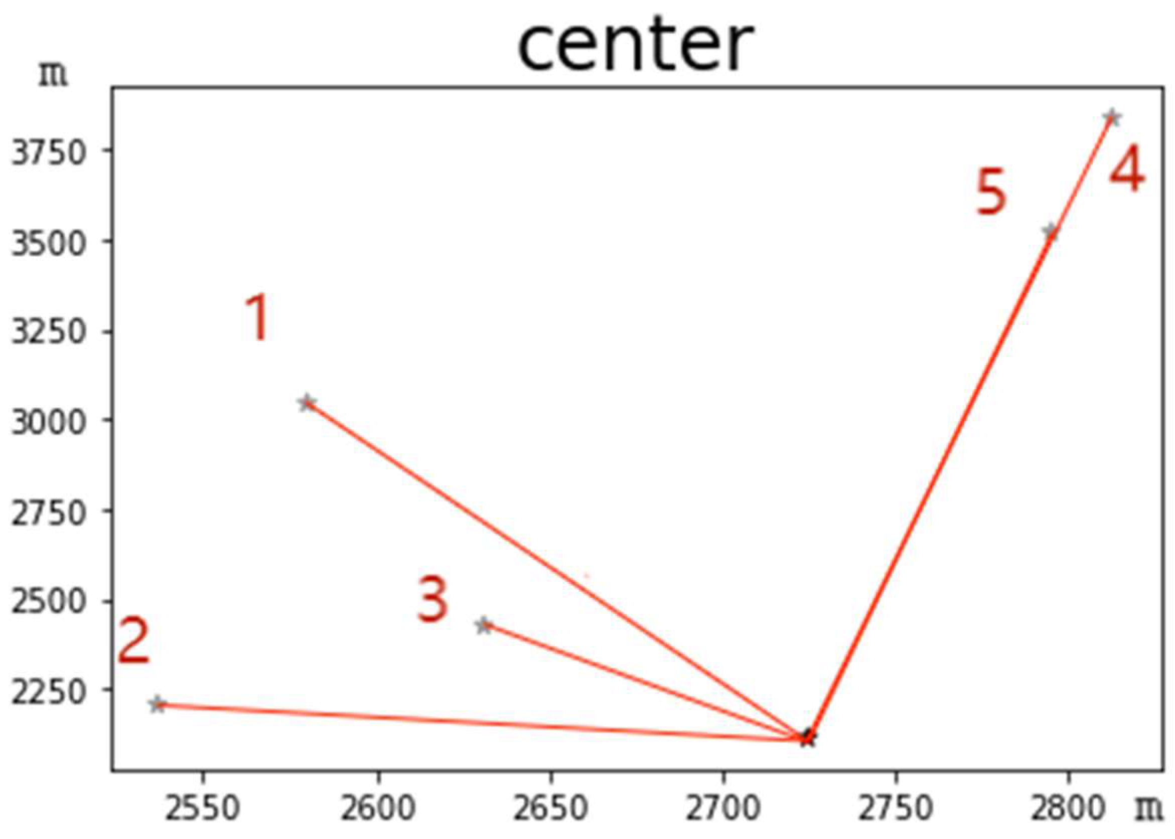
Constructing the spatial semantic relationship between sub-viewsheds and viewpoints reveals that sub-viewsheds are distributed in multiple viewing directions from the observation point. The direction and distance of each sub-viewshed from the viewpoint can be determined by calculating the azimuth attributes of the sub-viewsheds. The divided sub-viewsheds are labeled in
Figure 5 in the order of
Table 1 sub-viewshed numbers, the gray mark indicates the center point of each sub-viewshed, and the black mark indicates the observer point position. The abscissa and ordinate represent the relative distance between sub-viewsheds, starting from the origin position, considering the terrain accuracy, measured in meters. As can be seen from
Figure 5, the field of view is basically on one side of the observer. When the observer looks around, more viewsheds can be seen on the north side, with no visible areas in the opposite direction. The 3D simulated map of this terrain is shown in
Figure 7, where the observation point is on one side of the mountain ridge line, and the line of sight on the other side is blocked.
Table 1 displays the internal attributes of each sub-viewshed after partitioning, where the clustering partition has the highest number of visible points in sub-viewshed 1, followed by sub-viewshed 2, and the lowest number of views in sub-viewshed 3.
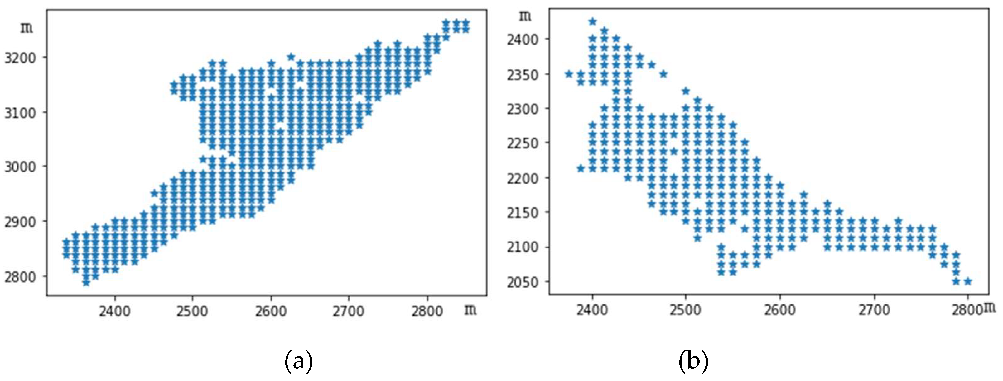
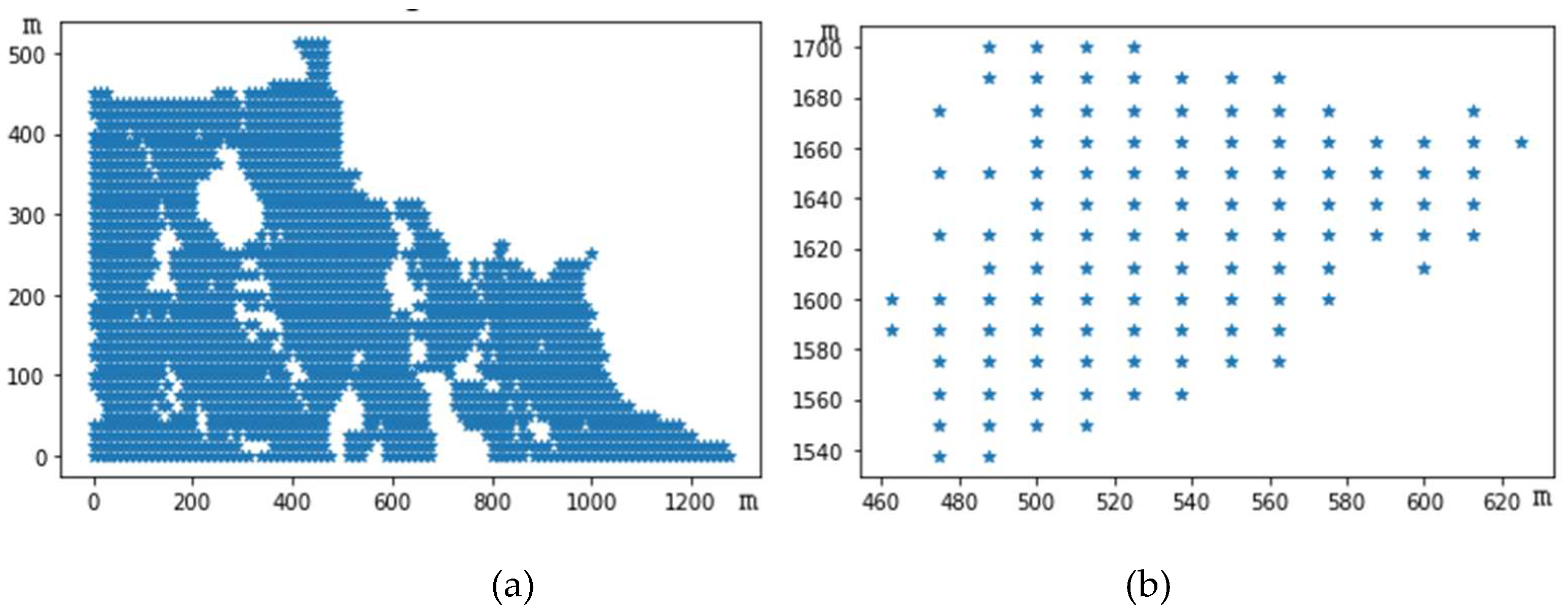
The shape of sub-viewshed 1 is shown in
Figure 6(a). There are 468 visible points within this sub-viewshed, with an area of 73,125 square meters and a density of 0.381. The distribution of visible points in this sub-viewshed is dense, indicating good view quality. The central point coordinates are [2580,3044], with an elevation value of 202.158 meters, situated at an intermediate altitude, and the visible points are distributed in the mountainside area. Sub-viewshed 1 is located at 99° from the observation point, approximately 952.081 meters from the observer. The distribution of visible points in the sub-viewshed is not concentrated enough, appearing linearly distributed. The average distance of the visible points is 200.36, and the sum of the central distances is 0.31. Due to the large number of visible points within the sub-area, the sum of the central distances is relatively small, and the lack of concentration in the distribution of visible points results in a more significant average distance of the view.
Sub-viewshed 2 contains 294 visible points, making it the second most populous area regarding the number of visible points. The shape is shown in
Figure 6(b). The average elevation of this sub-viewshed is 362.187 meters, which is at a relatively high altitude. The density of the sub-viewshed is 0.239. It is the closest view to the observer, approximately 211.691 meters away, located 154° from the observer. The horizontal distribution of visible points within the sub-viewshed spans considerably, with an average distance of 162.655. The sum of central distances is 0.4. Within the view range are areas without coverage by visible points, resulting in a relatively sparse distribution of visible points.
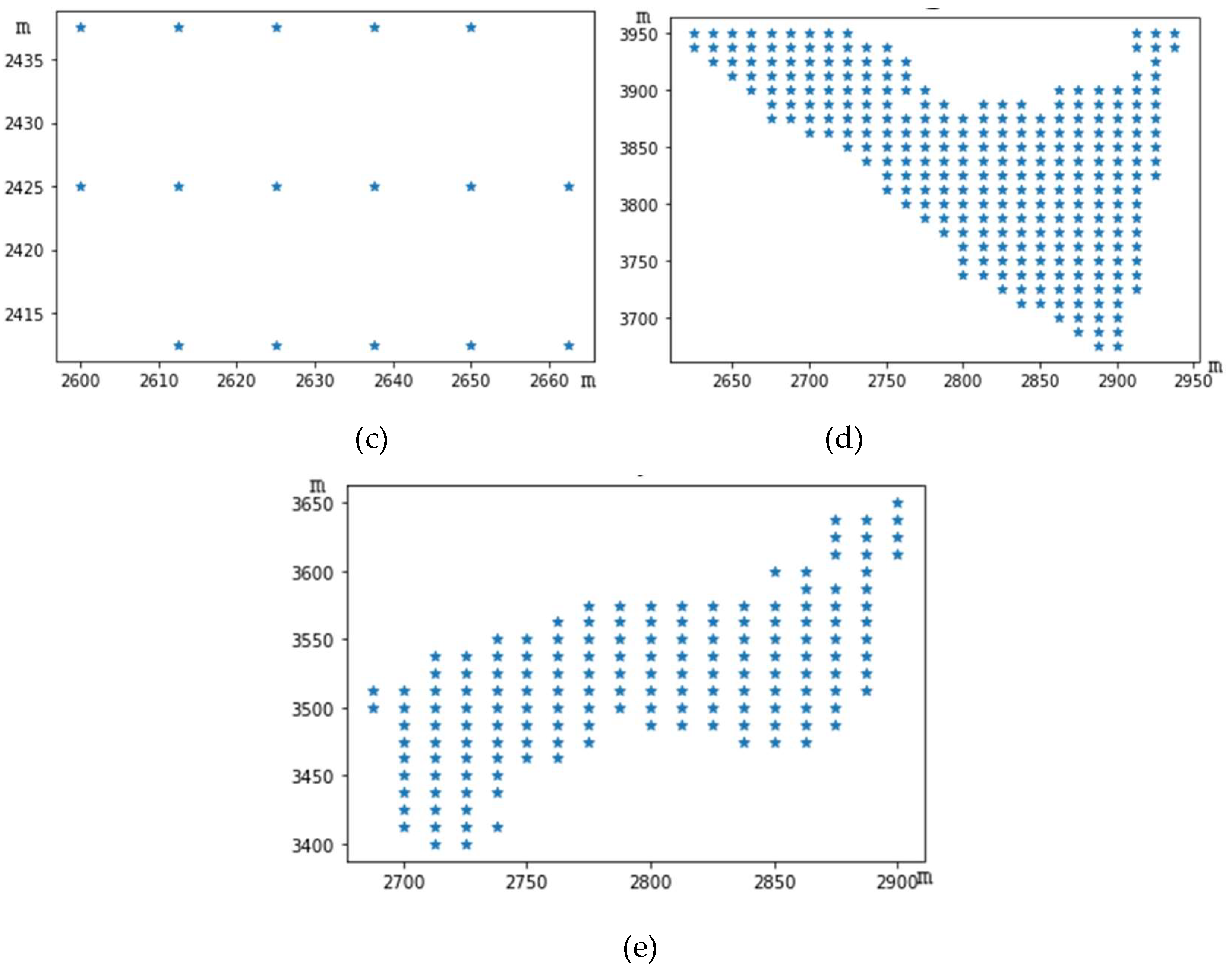
Sub-viewshed 3 has the most minor visible points, as shown in
Figure 6(c). The elevation of the center point of this viewshed is 286.562 meters, with 16 visible points. The viewshed is located 107° from the observation point, approximately 329.69 meters away, with an average distance of 27.428. This is the smallest average distance among all sub-viewsheds, and the sum of central distance is 1.277, which is the largest among all sub-viewsheds. Due to the small number of visible points in this sub-viewshed and their relatively concentrated distribution, each visible point is closely connected, forming a matrix-like distribution. This results in a situation where the average distance within the sub-viewshed is small while the sum of central distance is large.
The center of sub-viewshed 4 is located at [2813, 3838], with an average elevation of 84.425 meters, making it the lowest altitude among the five sub-viewsheds, as shown in
Figure 6(d). It has 275 visible points, a relatively high number distributed to this sub-viewshed, with a density of 0.224. This sub-view is the farthest from the observer at 1745.77 meters. The observer’s position is near the mountain top, while this sub-viewshed is located at the foot of the mountain. It is located at 87° of the observer. The shape distribution shows that the visible points are relatively concentrated, with an average distance of 132.128, and the sum of central distance is 0.351. Compared with sub-viewshed 2, it has fewer visible points but a smaller sum of central distance, indicating that the distribution of visible points in this viewshed is more concentrated and closer to the center than in sub-viewshed 2.
The elevation of Sub-viewshed 5 is 100.525 meters, which is the second lowest area compared to Sub-viewshed 4, as shown in
Figure 6(e). There are 160 visible points within this sub-viewshed, with a density of 0.13. Compared to the distribution of all visible areas, the number of viewpoints in this sub-viewshed could be sparser. According to the elevation, it is distributed at a lower altitude than the observation point. It is located at a distance of 1428.472 meters from the observation point, in the northeast direction by 87°. From
Table 1, it can be found that sub-viewsheds 4 and 5 are in the same direction as the observer; that is, when the observer looks in its northeast direction by 87°, they can simultaneously see the centers of sub-viewshed 4 and 5. The distance from these two sub-viewsheds to the observer is 1745.77 meters and 1428.472 meters. Since these three points are distributed on a straight line, it can be calculated that the center point distance between Sub-viewshed 4 and 5 is 317.298 meters, with an average distance of 101.837 meters, and the sum of the central distances is 0.465.
It can be observed that there are gentle terrains within each sub-viewshed, which is consistent with the characteristics of hilly terrains. The terrain does not fluctuate significantly and has a relatively mild slope. Purple Mountain, as a tourist attraction, has also been planned with multiple hiking routes for tourists to choose from, such as routes with steeper slopes and shorter durations, as well as routes with gentler slopes and longer durations. Except for Sub-viewshed 3, the average distances in the other sub-viewsheds are relatively large for two reasons: firstly, the visible points in the sub-viewshed are not concentrated, resulting in more considerable distances between two points; secondly, the number of visible points in the sub-viewshed is small. Compared with sub-viewshed 1 and 2, sub-viewshed 1 has a more significant number of visible points, differing by 174, but the difference in average distance is relatively small, about 38. This is due to the distribution of visible points in the sub-viewshed needing to be more concentrated, leading to more considerable distances between two visible points and thus increasing the average distance. From the shape distribution of these five sub-viewsheds, the distribution of visible points is relatively scattered and not concentrated enough, resulting in a larger average distance. At the same time, the sum of central distances is also an indicator reflecting the degree of concentration of visible points. The closer the distribution of visible points is to the center position, the smaller its value. Although sub-viewshed 1 has a more significant average distance, its maximum number of visible points results in a smaller sum of central distances; sub-viewshed 3, due to its smaller number of visible points, has a more enormous sum of central distances than the others.
Observing from two different positions north and south of Purple Mountain, the three-dimensional display of the viewshed division results is shown in
Figure 7,
Figure 7(a) is a view of the south side of the Purple Mountain, and
Figure 7(b) is a view of the north side of the Purple Mountain. Sub-viewshed 2 is distributed in the high-altitude area close to the mountain ridge line, and this viewshed has a wide range of visible points. Sub-viewshed 3 is located at the mountainside, which is also in a high-altitude area, but its elevation is lower than that of sub-viewshed 2, yet higher than sub-viewsheds 1, 4, and 5. Sub-viewshed 4 has the lowest altitude, near the foot of the mountain. Overall, sub-viewsheds 1, 4, and 5 are situated at relatively lower altitudes, with the region relatively flat.
Figure 7.
Three-Dimensional Diagram of Viewshed Partitioning.
Figure 7.
Three-Dimensional Diagram of Viewshed Partitioning.
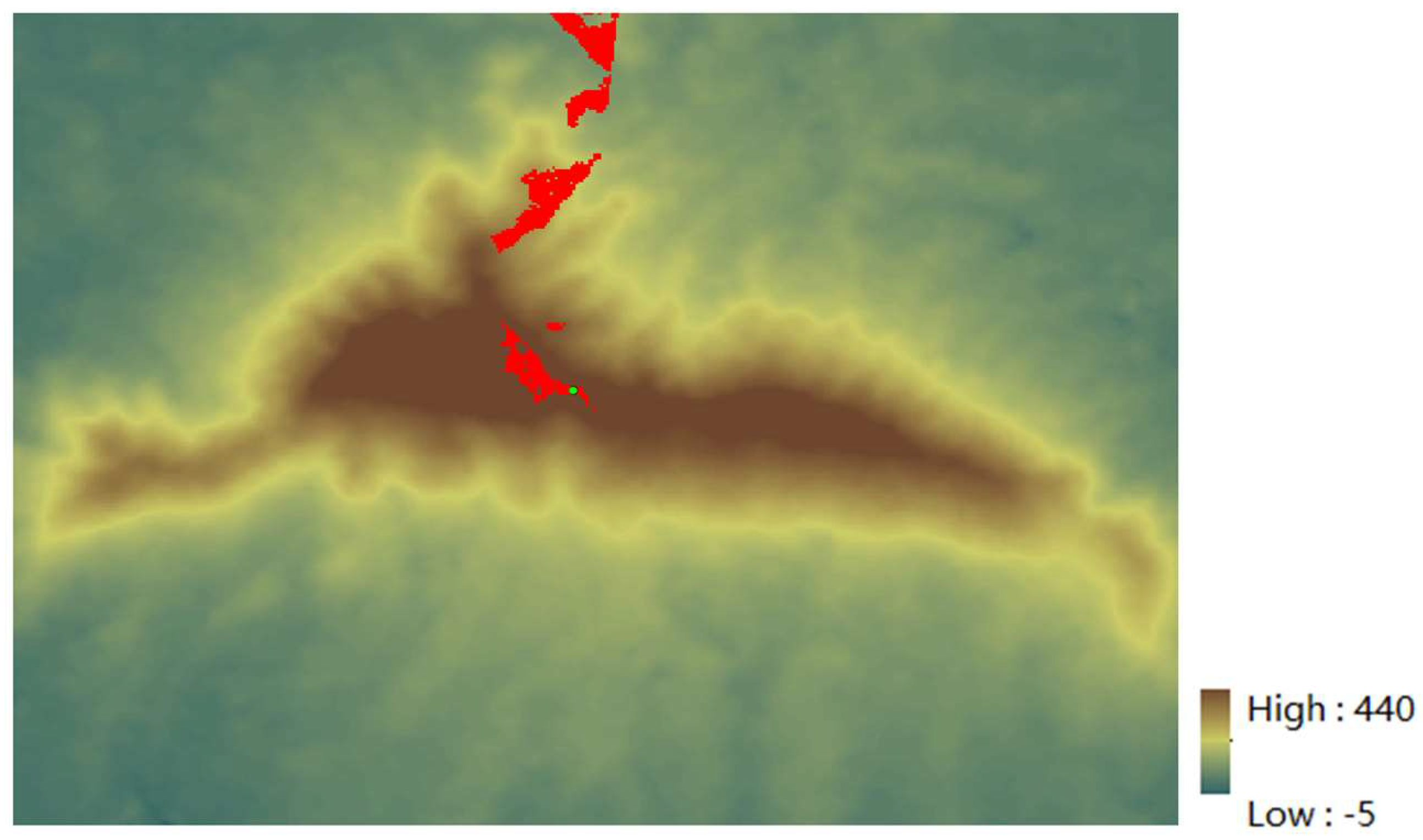
A new target point for observation is selected to perform viewshed analysis at this location. The resulting viewshed is depicted in
Figure 8. The observer’s coordinates are (118.855°E, 32.07°N) with an elevation value of 356 meters near the ridge line. A more extensive area is visible on one side of the ridge, demonstrating a broad field of view coverage distribution. Conversely, only a smaller area is observable on the other side of the hill.
Cluster analysis is performed on the terrain elevation within the range encompassed by the viewshed. Under the proposed methodology, suitable parameters are chosen for clustering. The viewshed is segmented into eight distinct sub-viewsheds, as
Figure 9(a) depicts.
Figure 9(a) highlights a notable disparity in the number of visible points, where each sub-viewshed encompasses within the viewshed partition.
Figure 9(b) delineates the spatial relationship between the center of each sub-viewshed and the observation point. The results of attribute value calculations within the sub-viewshed are presented in
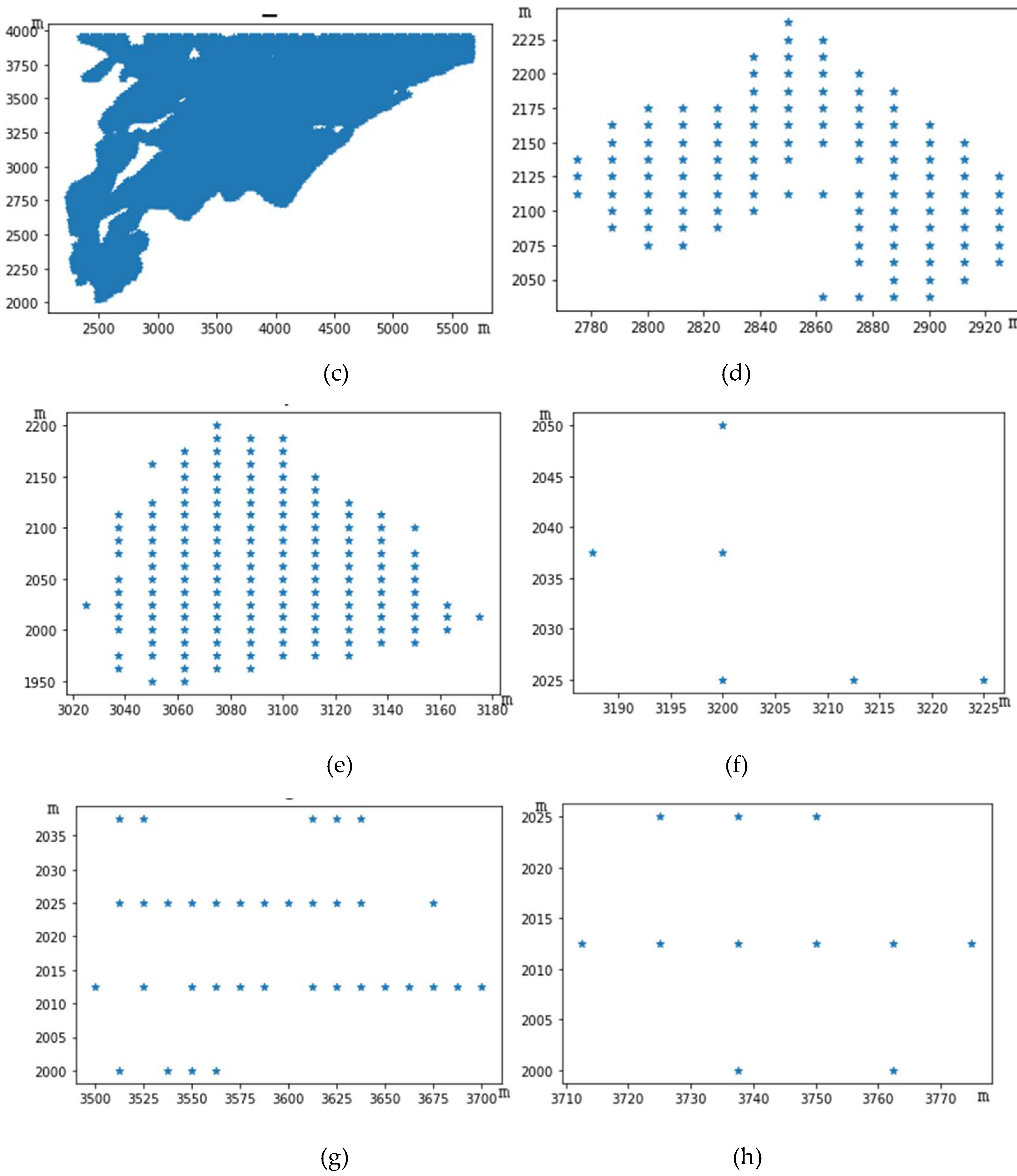
Table 2. Sub-viewshed 3 boasts the highest count of visible points, averaging an elevation of 103.687 meters. This is higher than that of sub-viewshed 1 but lower than others. This discrepancy can be attributed to the relatively flat terrain slope in this region, which lacks any steep inclines, leading to a concentration of more visible points totaling 17961. The density of the sub-viewshed is 0.8752, making it the sub-viewshed with the most visible points and the largest proportion among all visible points, yielding the best field of view quality. Sub-viewshed 3 is situated 89° from the observer at 1317.525 meters. This sub-viewshed encompasses a broad range. Due to the large number of visible points within sub-viewshed 3, the distribution of visible points in the area extends outward on both sides, resulting in the largest diameter involved and causing the maximum average distance within the sub-viewshed, which is 1144.833. Given many visible points in sub-viewshed 3, its sum of center distance is the smallest among all sub-viewsheds.
Sub-viewshed 1 is situated at the relative coordinate [457,188], as depicted in
Figure 10(a). The average elevation of sub-viewshed 1 stands at 25.098 meters, making it the lowest among all sub-viewsheds. The average elevation of visible points within this sub-viewshed is notably low, and the number of discernible grid points is relatively high. This suggests that sub-viewshed 1 is likely located in a predominantly flat area. Within its viewshed are 2112 visible points, ensuring a broad visual range. Sub-viewshed 1 is positioned 210° from the observer, at 3676.195 meters, making it the observer’s most distant viewshed. As illustrated in
Figure 8, sub-viewshed 1 is situated in a lower altitude corner area near the mountain’s base. At the same time, the observer is located near the ridge line at a higher altitude, resulting in a greater distance between them. The average distance of Sub-viewshed 1 is 409.653, indicating that the distribution of this viewshed is not sufficiently clustered. The distribution of visible points is either horizontal or vertical, failing to form a circular shape, which leads to larger attribute values.
The elevation of Sub-viewshed 2 is 230.628 meters, as shown in
Figure 10(b). As can be seen from
Figure 8, it is located at a relatively high altitude within the Purple Mountain branch hill, with 113 visible points in the viewshed, 3121.113 meters away from the observer, and 7° southwest of the observer. The average distance of sub-viewshed 2 is 76.167, and the sum of central distances is 0.494.
Sub-viewshed 4 is located at [2855,2128], as shown in
Figure 10(d). The elevation value of the sub-viewshed is 322.147 meters, with a total of 116 visible points and a density of 0.0057. The number of visible points is like that of sub-viewshed 2. It is 776.723 meters from the observation point and 8° northwest of the observer. The average distance of the sub-viewshed is 82.174, and the sum of central distances is 0.523. Compared with Sub-viewshed 2, these two sub-viewsheds have a similar number of visible points, both on the western side of the observer’s viewpoint, but differ in shape distribution. The difference between their average distance and the sum of central distance is not significant, indicating overall similarity in attribute values between the two sub-viewsheds.
From the perspective of directional attributes in sub-viewsheds, sub-viewsheds 4, 5, 6, and 7 are within a specific fixed visual range of the observer, and the distances between these sub-viewsheds are not far. When the observer looks in a specific direction, they can see these four sub-viewsheds simultaneously. Sub-viewshed 5 is located 4° northwest of the observer, at 535.664 meters; sub-viewshed 6 is located 1° northwest of the observer, at 421.76 meters; sub-viewshed 7 is located 10° southwest of the observer, at a distance of 36.363 meters, which is also the closest sub-viewshed to the observer. To the observer, the visual angles of these sub-viewsheds form an angle of 18 degrees. With attention concentrated, the human eyes’ visible field of view is approximately 25 degrees. Therefore, when viewing from a certain angle, the observer can focus their attention and simultaneously see these four sub-viewsheds. Although sub-viewshed 2 is also within this visual angle range, due to its great distance, the visual effect of sub-viewshed 2 will decrease when the observer is looking closely.
The shape of each sub-viewshed division is shown in
Figure 10. The sub-viewshed with the highest number of visible points is sub-viewshed 3, while the one with the least number of visible points is sub-viewshed 6, which has only 6 visible points. This sub-viewshed is at a higher altitude, with an elevation value of 329.334 meters. The distribution of visible points is shown in
Figure 10(f). As can be seen from the figure, the visible points are distributed within a 3×4 grid unit, and this viewpoint is near the ridge line of Purple Mountain, where there exists flat land within the viewpoint.
The results reflected from the internal attribute values suggest that the distribution of visible points in sub-viewsheds 7 and 8 is relatively similar. The elevation values of these two sub-viewsheds differ slightly, with the number of visible points in sub-viewshed 7 being approximately three times that of sub-viewshed 8. This is also reflected in the average distance attributes, which are nearly three times as much. Due to the more significant number of visible points in sub-viewshed 7, the sum of central distance is slightly smaller compared to sub-viewshed 8. As can be seen from
Figure 10, both sub-viewsheds 7 and 8 exhibit a horizontal stripe distribution.
The average distance attributes of sub-viewshed 2 and 7 differ slightly, but sub-viewshed 2 has 113 visible points, while sub-viewshed 7 has only 35. This difference in the number of visible points is due to the distribution of visible points in the two sub-viewsheds. The distribution of visible points in sub-viewshed 2 is more concentrated, resulting in a smaller distance between any two visible points within the view. On the other hand, the distribution of visible points in sub-viewshed 7 is linear, with no concentration, leading to a large distance between any two points within the view. This results in a slight difference in the average distances between the two sub-viewsheds. It also reflects that the distribution of sub-viewshed 7 is sparser than that of sub-viewshed 2, with a more concentrated distribution of visible points in sub-viewshed 2.
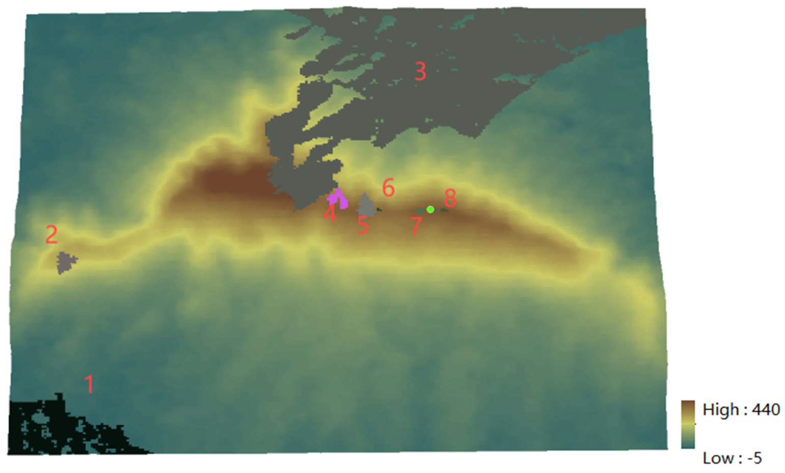
Figure 11 shows the three-dimensional graph of terrain after clustering partition. The figure shows that the visible points in sub-viewshed 3 involve a larger area, from the bottom of the mountain to the slope and finally to the ridge line position. The distance between any two adjacent visible points within this sub-viewshed is less than or equal to 18 meters; thus, they are clustered together. This feature also reflects the relatively flat characteristics of the terrain in this sub-viewshed. Based on this sub-viewshed, path planning for mountain climbing roads can be conducted so that tourists will not walk to steep slopes during their ascent.
The observation point is located on the north side of the ridge line, allowing it to see a larger area on one side. In contrast, the other side is not fully visible due to obstructions in the line of sight, and only a tiny part of the distance can be seen. The figure shows that sub-viewsheds 4, 5, 6, 7, and 8 are distributed along the ridge line. A walking path can be planned based on these sub-fields for tourists to enjoy. If the position of the observation point is set as an observation post or target scenic area, all sub-viewsheds can simultaneously see this target point.